High Performance Computing for the Reduced Basis Method. Application to Natural Convection

(1)

S. Descombes, B. Dussoubs, S. Faure, L. Gouarin, V. Louvet, M. Massot, V. Miele, Editors

HIGH PERFORMANCE COMPUTING FOR THE REDUCED BASIS METHOD.

APPLICATION TO NATURAL CONVECTION

E. Schenone

1,2

, S. Veys

3

et C. Prud’homme

4

Abstract. In this paper, we are interested in applying the reduced basis methodology (RBM) to steady-state natural convection problems. The latter has applications in many engineering domains and being able to apply the RBM would allow to gain huge computation savings when querying the model for many parameter evaluations. In this work, we focus on the order reduction of the model — in particular the handling of the non-linear terms, — as well as the design of the RBM computational framework and the requirements on high performance computing to treat 3D models using_Feel++, a C++ open source library to solve partial differential equations. Numerical experiments are presented on 2D and 3D models.

Introduction

Nowadays, in many application fields, engineering problems require accurate, reliable, and efficient evaluation of quantities of interest. Often, these quantities of interest depend on the solution of a parametrized partial

differential equation where the — e.g. physical or geometrical — parameters are inputs of the model and

the evaluation of quantities of interest are outputs — e.g. average values. In a real-time or many-query context, the reduced basis method (RBM) offers a rapid and reliable evaluation of the input-output relationship (see [PRV+02,VPP03,VPRP03,PP04,QRM11,RHP07] for the methodology) for a large class of problems.

In this paper, we are interested in studying the RBM applied to steady-state natural convection problems parametrized by the Grashof and Prandtl numbers, see also [VP05,Yan12]. Natural convection has applications in many engineering domains and being able to apply the RBM would allow to gain huge computation savings when querying the model the reduced model for many parameter evaluations. In this work, we focus on the order reduction of the model — in particular the handling of the non-linear terms, — as well as the design of the RBM computational framework and the requirements on high performance computing (HPC) to treat 3D models. Even though the model considered remains simple with respect to industrial applications, we tackle some of the main difficulties namely order reduction and computational costs. In this work, we underly the difficulties linked to the resolution of non-linear problems in a reduced space. We detail a projection technique that can be applied to any second order problem and that allows to solve it in the reduced space, without any projection onto the FE space. To the authors knowledge, previous works on the RB applied to non-linear steady Navier-Stokes equations concentrate on the choice of the basis and on error estimators, see [VP05,Yan12]. We propose here a reduced order method that can be applied to any non-linear problem and that does not depend on the choice of the basis.

1 _{Laboratoire Jacques Louis Lions, UPMC, 4 Place Jussieu, 75005 Paris, France}

2 _{Inria Paris-Rocquencourt, Domaine de Voluceau B.P. 105, 78153 Le Chesnay Cedex, France -}_{[email protected]}

3_{Laboratoire Jean Kuntzmann, Universit´}_{e Joseph Fourier Grenoble 1, BP53 38041 Grenoble Cedex 9, France -}_{[email protected]} 4_Universit´_{e de Strasbourg, IRMA UMR 7501, 7 rue Ren´}_{e-Descartes, 67084 Strasbourg Cedex, France -}_{[email protected]}

©EDP Sciences, SMAI 2013

(2)

In order to solve Finite Elements (FE) or Reduced Basis (RB) problems, we use an open-source library called Feel++ for Finite Element Embedded Library and Language in C++ ( [PCD+12,Pru06] ). Feel++ is a library to solve problems arising from partial differential equations (PDEs) with Galerkin methods, standard or generalized, continuous or discontinuous, from 1D to 3D, for low to high order approximations (including

geometry). Among the many other _Feel++features, it provides a seamless programming environment with

respect to parallel computing using MPI, see section 4.1. _Feel++ enjoys an implementation of the RBM,

see [DVTP13], which can deal with a wide range of problems: elliptic or parabolic models, coercive or non-coercive models, linear or non-linear models. It can handle coupled non-linear multiphysic problems such as the thermo-electric problems in [VDPT12,VCD+12]. It is important that such an environment hides as many implementation details as possible and let the user worry only about his/her model and the high level aspects of the FEM and RBM.

The organisation of the paper is as follows: in section 1 we describe the 2D and 3D steady-state natural convection models; in section 2, we present the finite element discretization and the solution strategy; in section 3, we apply the RBM and focus in particular on the non-linear terms handling; in section 4, we present the computational framework for FEM and RBM as well as some implementation aspects; finally in section 5, we display some numerical experiments in 2D and 3D.

1. _{Problem setting}

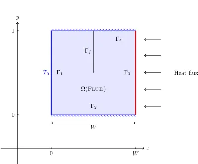
We start with the description of a standard natural convection model. We consider a heated fluid in a squared or cubical cavity, the fluid circulates towards the low temperature under the action of density and gravity differences. We introduce the adimensionalized steady-state incompressible Navier-Stokes equations coupled with the heat equation and we consider the problem in a two and a three dimensional tank, see e.g. Figure1: find (u, p, T) such that



                  

                  

u· ∇u+∇p−√1

Gr4u = Te2 , in Ω

∇ ·u = 0 , in Ω

u· ∇T −√ 1

GrP r4T = 0 , in Ω

u = 0 , on∂Ω T = 0 , on Γ1 ∂T

∂n = 0 , on∂Ω\(Γ1∪Γ3) ∂T

∂n = 1 , on Γ3.

(1)

where Ω ⊂Rd, d= 2,3,u,pand T are respectively the adimensionalized velocity, pressure and temperature,

Gr andP r are the Grashof and the Prandtl numbers, ande2 is the inward-pointing normal vector of a border Γ2⊂∂Ω. The 2D domain consists in a rectangular tank of height 1 and lengthW, in the 3D case we consider a rectangular cuboid of height 1, length W and depth 1. A heat flux is imposed on the “right” border Γ3 while the temperature is fixed on the “left” border Γ1 and the remaining walls are insulated. Similar boundary conditions apply in 3D. No-slip boundary conditions are set for the fluid velocity in the tank.

(3)

x

0 W

y

0 1

Γ1

Γ2

Γ3

Γ4

Ω(Fluid)

W Γf

T0 Heat flux

Figure 1. Geometry of the 2D model. Consider an extrusion of this geometry in 3D case is the extrusion in z axis of length 1.

2. Finite element formulation

In this section, we write the weak Galerkin formulations associated to (1) and we propose an iterative method to solve this problem in case of FE space and a resolution with the RBM.

The weak formulation associated to problem (1) writes

a(u,u,v)−b(p,v) +√1

Grc(u,v)−d(T,v) = 0 ,∀v∈V b(q,u) = 0 ,∀q∈Q e(T,u, ξ) +√ 1

GrP rg(T, ξ)− 1

√

GrP rh(ξ) = 0 ,∀ξ∈Ξ

(2)

where V ≡ [H1

0(Ω)]d, Q ≡ L2(Ω), Ξ ≡ {ξ ∈ H1(Ω) s.t. ξ|Γ1 = 0}, and we define the tri-linear forms a :

V ×V ×V →Rande: Ξ×V ×Ξ→Ras

a(u,w,v) =

Z

Ω

(w· ∇u)·v, ∀u,w,v∈V (3)

e(T,v, ξ) =

Z

Ω

(v· ∇T)ξ, ∀v∈V, T, ξ∈Ξ (4)

the bi-linear formsb:Q×V →_R,c:V ×V →_R,d: Ξ×V →_Randg: Ξ×Ξ→_Ras

b(q,v) =

Z

Ω

q∇ ·v, ∀v∈V, q∈Q (5) c(w,v) =

Z

Ω

∇w:∇v, ∀w,v∈V (6)

d(ξ,v) =

Z

Ω

ξe2·v, ∀v∈V, ξ∈Ξ (7) g(T, ξ) =

Z

Ω

(4)

and the linear operatorh: Ξ→_Ras

h(ξ) =

Z

Γ3

ξ, ∀ξ∈Ξ. (9)

We introduce now a FE discretization of (2). We define the discrete spacesVh ⊂V, Qh ⊂Q, Ξh ⊂Ξ and

the associated Galerkin projection of the solution (u, p, T) of (2) by

Vh≡span{φ1, . . . ,φNu} , u'

Nu

X

j=1 ujφj

Qh≡span{ψ1, . . . , ψNp} , p'

Np

X

j=1 pjψj

Ξh≡span{ξ1, . . . , ξNT} , T '

NT

X

j=1 Tjξj.

The discrete formulation of (2) now reads

Nu

X

i,j=1

uiuja(φi,φj,φk1) + Nu

X

i=1 1

√

Gruic(φi,φk1)−

Np

X

i=1

pib(ψi,φk1)− NT

X

i=1

Tid(ξi,φk1) = 0 , k1= 1, . . . , Nu

Nu

X

i=1

uib(ψk2,φi) = 0, k2= 1, . . . , Np (10) NT X i=1 Nu X j=1

Tiuje(ξi,φj, ξk3) +

1 √ GrP r NT X i=1

Tig(ξi, ξk3)−

1

√

GrP rh(ξk3) = 0, k3= 1, . . . , NT

Due to its strong non-linearities, when the Grashof or Prandtl numbers are high, a robust iterative method is required to solve this problem. We apply here a Newton Method. For a given parameter µ= (µ1, µ2) = (Gr−1/2, P r−1) and an initial guess (u0, p0, T0), at each Newton sub-iteration n = 1, . . . , nmax we look for

(un+1, pn+1, Tn+1)∈RNu_× RNp_×

RNT _{such that}

J(un, pn, Tn;µ)

(un+1, pn+1, Tn+1)−(un, pn, Tn)

=R(un, pn, Tn;µ) (11)

whereJ =J(u, p, T;µ) is the Jacobian matrix,R=R(u, p, T;µ) is the residual vector.

In the case of problem (10) the terms of the Jacobian matrix can be easily calculated. For each row k1 = 1, . . . , Nu they write

Jk1i(u, p, T;µ) = Nu

X

j=1

uja(φi,φj,φk1) + Nu

X

j=1

uja(φj,φi,φk1) +µ1c(φi,φk1), i= 1, . . . , Nu

Jk1Nu+i(u, p, T;µ) =−b(ψi,φk1), i= 1, . . . , Np

Jk1Nu+Np+i(u, p, T;µ) =−d(ξi,φk1), i= 1, . . . , NT

(12)

for all rowk2=Nu+k,k= 1, . . . , Np

Jk2i(u, p, T;µ) =b(ψk,φi), i= 1, . . . , Nu

Jk2Nu+i(u, p, T;µ) = 0, i= 1, . . . , Np Jk2Nu+Np+i(u, p, T;µ) = 0, i= 1, . . . , NT

(5)

and for all linek3=Nu+Np+k,k= 1, . . . , NT

Jk3i(u, p, T;µ) = NT

X

j=1

Tje(ξj,φi, ξk), i= 1, . . . , Nu

Jk3Nu+i(u, p, T;µ) = 0, i= 1, . . . , Np Jk3Nu+Np+i(u, p, T;µ) =

Nu

X

j=1

uje(ξi,φj, ξk) +µ1µ2g(ξi, ξk), i= 1, . . . , NT.

(14)

In the same way, each term of the residualR(u, p, T;µ)∈RNu+Np+NT _{can be calculated by} Rk(u, p, T;µ) =−a(u,u,φk) +b(p,φk)−µ1c(u,φk) +d(T,φk), k= 1, . . . , Nu

RNu+k(u, p, T;µ) =−b(ψk,u), k= 1, . . . , Np RNu+Np+k(u, p, T;µ) =µ1µ2h(ξk)−e(T,u, ξk)−µ1µ2g(T, ξk), k= 1, . . . , NT

Remark 2.1. For high Gr andP rnumbers the Newton method might be insufficient. We propose in that case to use the continuation algorithm 1. Note however that we do not apply this continuation method in results presented below.

Algorithm 1Continuation strategy for highGr andP r numbers. Fix parametersGr andP r

Fix minimal values of parametersGrmin = 1 andP rmin= 10−2

Fix tolerancetoland max number of iterationnmax for Newton

Calculate number of intermediary parameters:

N = maxn1; max

dlog(Gr/Grmin)e),d(log(P r/P rmin)e

o

fori=1:Ndo

Logarithmic scale for intermediary parameters: Gr(i) =exp{log(Grmin) +i(log(Gr/Grmin))/N)

P r(i) =exp{log(P rmin) +i(log(P r/P rmin))/N)

Fix Newton initial guessu0=uold

while||R|| ≥tol orn≤nmax do

findun _s.t. _J₍_un−1₎₍_un₋_un−1_{) =}_R₍_un−1₎ end while

uold=un

end for

return Solutionu=un

3. Reduced basis formulation

(6)

3.1. Reduced Basis for a general quadratic problem

We now turn to the generalization of the RBM to a quadratic problem, in abstract form it reads

a(u, u, v;µ) +b(u, v;µ) =f(v;µ), ∀v∈V (15)

where the solution is u=u(µ)∈V, µ∈RQ indicatesQscalars parameters, V is an Hilbert space defined on a domain Ω⊂Rd, withd= 1,2,3,a:V ×V ×V →Ris a tri-linear form, b:V ×V →Ris a bi-linear form, andf :V →Ris a linear operator.

We first introduce the FE approximation of (15) that leads to the RB approximation. The RB formulation of the general problem (15) applies then to (2).

Let us define a FE space VN ≡span{v1, . . . , vN} ⊂V, and the approximated solution of (15) as

u(µ)' N X

i=1

ui(µ)vi

then the discrete formulation of (15) writes

N X

i,j=1

uiuja(vi, vj, vk;µ) + N X

i=1

uib(vi, vk;µ) =f(vk;µ), ∀k= 1, . . . ,N (16)

where the solutionu=u(µ) = [u1· · ·uN]T ∈RN for each parameterµ∈RQ.

In order to describe the RB approximation applied to problems such as (15), we need to define some discrete objects. In particular, we introduce the tensorA=A(µ)∈RN ×N ×N, the matrixB =B(µ)∈RN ×N, and the vectorf =f(µ)∈_RN _{defined by}

(A)ijk=a(vi, vj, vk;µ), (B)ki=b(vi, vk;µ), (f)k=fk=f(vk;µ)

fori, j, k= 1, . . . ,N. Note that the tensorAcan be considered as a vector of matrices,i.e.for eachk= 1, . . . ,N, we define the matrixAk =Ak(µ)∈RN ×N as (Ak)ij = (A)ijk, i, j = 1, . . . .N. Using this notation (16) now

reads

uTAku+ (Bu)k =fk, ∀k= 1, . . . ,N (17)

where (Bu)k andfk are respectively thek-th term of vectorsBuandf.

As described in Section 2 we can treat the non-linearity of the first term in (17) using a Newton Method. For a given parameterµ∈RQ, each iterationn= 1,2, . . .of the Newton algorithm reads

Jrow(k)(un;µ)(un+1−un) =Rk(un;µ), ∀k= 1, . . . ,N (18)

where Jrow(k)(un;µ)∈RN andRk(un;µ) are respectively the k-th row of the Jacobian matrixJ =J(u;µ)∈

RN ×N and thek-th term of the residualR=R(un;µ)∈RN defined by

Rk(un;µ) =fk−(un)TAkun−(Bun)k, k= 1, . . . ,N. (19)

(7)

Now, we just need to calculate the Jacobian matrixJ =J(u;µ). We can write each of its elements as

Jki(u) =

∂a ∂ui

(u,u, vk) +

∂b ∂ui

(u, vk)−

∂f ∂ui

(vk) =

= N X l=1 N X j=1 ∂ ∂ui

uluja(vl, vj, vk)

+ N X j=1 ∂ ∂ui

b(vj, vk)uj

= = N X l=1 N X j=1 ∂ ∂ui

ulAljkuj+ N X

j=1 ∂ ∂ui

Bkjuj=

=

N X

j=1

ujAjik+ N X

j=1

Aijkuj+Bki. (20)

In generalAis never assembled as it is of sizeN3_{, where}_N _{is the dimension of the underlying discretization} space. If this is indeed the case for FE discretization, recall however that here we deal with reduced order approximation which enables the computation of A explicitly. Let us then introduce a reduced space VN =

span{ϕ1, . . . , ϕN}, withN N and define the projectionue=eu(µ)∈R

N_{of the solution}_u_in_V N as e u= N X i=1 e

uiϕi= ΦTu, (21)

where Φ = [ϕ1. . . ϕN]∈RN ×N, Φji= ˆϕi,j= (ϕi, vj)VN, the coefficientseui are

e

ui= (u, ϕi)VN = (u,

N X

j=1 ˆ

ϕi,jvj)VN =

N X

j=1 ujϕˆi,j

and (·,·)VN is the scalar product associated toVN.

We observe that the Newton method defined in (18) is in fact generic with respect to the discrete spaces and that we can replaceVN by VN which corresponds to projections of the terms in (18) ontoVN. We now prove

this statement.

Following the procedure of (21) we start by defining the projection of the source termf asef =ef(µ)∈_RN

ef = ΦTf, (22)

then the matrix Be=Be(µ)∈RN×N as well is the projection of B into the reduced spaceVN

e

B= ΦTBΦ, (23)

and finally we denote the reduced size tensor Ae = Ae(µ) ∈ RN×N×N. We now prove that it is in fact the

projection of the tensorA∈RN ×N ×N inVN

e

Aijk =a(ϕi, ϕj, ϕk) = N X

l,m,h=1 ˆ

ϕi,lϕˆj,mϕˆk,ha(vl, vm, vh) =

=

N X

l,m,h=1 ˆ

ϕi,lϕˆj,mϕˆk,hAlmh= N X

h=1 ˆ

ϕk,h(ΦTAhΦ)ij = N X

h=1 ˆ

(8)

i, j, k= 1, . . . , N, whereAek= ΦTAkΦ is the projection ofAk∈RN ×N inVN for allk= 1, . . . ,N. Let us define

the tensorial product?:_RN _×

RN →Ras

aT ?(bTAc) :=

N X

h=1

ah(bTAhc), ∀a,b,c∈RN,∀A∈RN ×N ×N. (25)

Then

e

Aijk = N X

h=1 ˆ

ϕk,h(ϕTi Ahϕj) =ϕTk ?(ϕ T

i Aϕj), i, j, k= 1, . . . , N. (26)

Using equations (23) and (26) we obtain the projection of the Jacobian Je∈ RN×N at each iteration n=

1,2, . . ., and it reads

e

Jik(eu

n_;_µ_{) = (}

e

Ak|col(i))Tue

n_{+ (}

e

Ak|row(i))eu

n₊

e

Bik (27)

where Aek|col(i) = [Aejik]Nj=1 ∈ RN is thei-th column of the matrix Aek for each k = 1, . . . , N and Aek|row(i) = [Aeijk]Nj=1 ∈RN is thei-th row of the matrixAek for eachk= 1, . . . , N. If we use the tensorial product defined

by (25) we simply write

e

Ak|col(i)=

h

ϕT_k ?(ϕT₁Aϕi) · · · ϕTk ?(ϕ T NAϕi)

i

e

Ak|row(i)=

h

ϕT_k ?(ϕT_iAϕ1) · · · ϕT_k ?(ϕT_i AϕN)

i

i, k= 1, . . . , N. Similarly, each term of the reduced residualRe=Re(u_e;µ)∈_RN reads

e

Rk(_eun;µ) =fek−(u_en)TAek_eun−(Be_eun)k, k= 1, . . . , N. (28)

3.2. Application to heat convection problem

Let us now apply this reduction technique to the natural convection problem introduced in Section 2. The FE formulation of each sub-iterationn= 1, . . . , nmax of the Newton Method applied to equations (2) writes

J(un, pn, Tn)

(un+1, pn+1, Tn+1)−(un, pn, Tn)

=R(un, pn, Tn) (29)

with Jacobian and residual terms defined as in Section2. In order to apply the technique described in the pre-vious paragraph, we introduce matrices and tensors associated to (10). We define the tensorsA∈_RNu×Nu×Nu andE∈_RNT×Nu×NT _as

A= [Aijk, i, j, k= 1, . . . , Nu], (Ak)ij=Aijk =a(φi,φj,φk)

E= [Eijk, i, k= 1, . . . , NT, j= 1, . . . , Nu], (Ek)ij=Eijk =e(ξi,φj, ξk)

the matricesB∈RNp×Nu_,_C_∈

RNu×Nu_, _D_∈

RNu×NT_,_G_∈

RNT×NT _as

B= [Bij, i= 1, . . . , Nu, j= 1, . . . , Np], Bij =b(ψj,φi)

C= [Cij, i, j= 1, . . . , Nu], Cij=c(φj,φi)

D= [Dij, i= 1, . . . , Nu, j= 1, . . . , NT], Dij=d(ξj,φi)

G= [Gij, i= 1, . . . , NT], Gij=g(ξj, ξi)

and the vectorH ∈_RNT _as

(9)

Then, using notation introduced in Section3.1, the Jacobian matrix writes

J(u, p, T;µ) =





JN l1₍_u_{) +}_µ1C ₋_B ₋_D

BT 0 0

JN l2₍_T₎ ₀ _JN l3₍_u_{) +}_µ1µ2G



 (30)

where each element of the non-linear submatricesJN l1₍_u_),_JN l2₍_T_),_JN l3₍_u_{) are}

JN l1 ki (u) =

Nu

X

j=1

((Ak)ij+ (Ak)ji)uj= ((Ak|col(i))T+ (Ak|row(i)))u, k, i= 1, . . . , Nu

JN l2 ki (T) =

NT

X

j=1

(Ek)ijTj = (Ek|row(i))T , k= 1, . . . , NT, i= 1, . . . , Nu (31)

JN l3 ki (u) =

Nu

X

j=1

(Ek)jiuj = (Ek|col(i))Tu, k, i= 1, . . . , NT

whereas each element of the residual vector of the Newton algorithm (11) writes

Rk(u, p, T;µ) =−uTAku+Brow(k)p−µ1Crow(k)u+Drow(k)T , k= 1, . . . , Nu

Rk(u, p, T;µ) =−(Bcol(k))Tu , k=Nu+ 1, . . . , Nu+Np (32)

Rk(u, p, T;µ) =µ1µ2Hk−uTEkT−µ1µ2Grow(k)T

To apply efficiently the RB methodology, a key ingredient is the affine decomposition of the terms in the Newton Method which is readily available for our problem. The Jacobian matrix writes as

J(u, p, T;µ) =

QJ

X

q=1

θ_Jq(µ)Jq(u, p, T) (33)

where for the considered exampleQJ= 4 and the coefficientsθJ are

θ_J1(µ) =µ1=√1

Gr, θ 2

J(µ) =µ1µ2=

1

√

GrP r, θ 3

J(µ) =θ

4

J(µ) = 1. (34)

Each sub-matrix can be described using the notation introduced above

J1(u, p, T) =





C 0 0

0 0 0



, J2(u, p, T) = 



0 0 0

0 0 G



, (35)

J3(u, p, T) =





0 −B −D BT 0 0

0 0 0



, J4(u, p, T) = 



JN l1₍_u₎ ₀ ₀

0 0 0

JN l2₍_T₎ ₀ _JN l3₍_u₎



.

As to the residual, it is readily decomposed as

R(u, p, T;µ) =

QR

X

q=1

(10)

withQR= 3 terms, we have

θ1_R(µ) =µ1= 1

√

Gr, θ 2

R(µ) =µ1µ2= 1

√

GrP r, θ 3

R(µ) = 1 (37)

and

R1(u, p, T) =





−Cu

0 0



 , R2(u, p, T) = 



0 0 H−GT



 , (38)

R3₍_{u, p, T}_{) =}





−(uTAku)Nk=1u +Bp+DT BTu

−((uTEkT)T)Nk=1T



.

The last step consists in projecting these equations in a reduced space. As shown for the general problem (15), the reduced Newton method at each iterationn= 1, . . . , nmax writes

e

J(u_en,p_en,Ten) h

(_eun+1,p_en+1,Ten+1)−(_eun,p_en,Ten) i

=Re(u_en,_epn,Ten) (39)

where the ∼ indicates the projection onto the reduced spaceVN. The computation of vectors and matrices

is done in a ”classical” way, the terms are calculated in the FE space VN and projected into the reduced one

by the matrix Φ defined by the basis function. Each basis function is the solution of problem (10) for a fixed parameterµ, possibly orthonormalized. For tensors A andE a different approach is needed because of their high dimensions.

Let us consider a general tensor A ∈ RN3 defined by a trilinear form a : V3

N → R, Aijk = a(vi, vj, vk),

i, j, k = 1, . . . ,N as in problem (15). Its projection on a reduced space VN = span{ϕ1, . . . , ϕN}, as shown in

Section3.1, is defined byAe∈RN

3

,Aeijk=ϕTk?(ϕTiAϕj),i, j, k= 1, . . . , N. We observe thatAeijk=a(ϕi, ϕj, ϕk)

whereϕi, ϕj, ϕk ∈VN.

Let us then define an hybrid tensor Λ∈_RN ×N ×N _{whose elements are}

Λijk = (Λk)ij =a(vi, vj, ϕk), (40)

i, j= 1, . . . ,N,k= 1, . . . , N. We can then use this tensor to redefine the reduced tensorAe

e

Aijk=a(ϕi, ϕj, ϕk) = N X

l,m=1 ˆ

ϕi,lϕˆj,ma(vl, vm, ϕk) =

=

N X

l,m=1

ΦliΦmj(Λk)lm= (ΦTΛkΦ)ij. (41)

So, we proved that

e

Ak= ΦTΛkΦ. (42)

That implies that we can calculate onlyN matrices Λk,k= 1, . . . , N, and project them into the reduced space

to obtain the reduced tensorAe.

(11)

4. Computational framework

In this section we give an overview of the computational framework and its implementation to solve the heat convection problem introduced in section 2. All the routines described are part of the FE or RB frameworks of Feel++library and available inFeel++source code. We first introduce the main principles of Feel++, then we illustrate the FE implementation of problem (1) and finally we introduce the associated RB framework.

4.1. Feel++ principles and design

Feel++ is a C++ library that provides a clear and easy to use interface to solve complex PDE systems. It aims at bringing the scientific community a tool for the implementation of advanced numerical methods and high performance computing.

Feel++ relies on a so-called Domain Specific Embedded Language (DSEL) designed to closely match the Galerkin mathematical framework. In computer science DS(E)Ls are used to partition complexity. In_Feel++ the DSEL splits low level mathematics and computer science on one side, and high level mathematics as well as physical applications to the other side. This difference between disciplines is reflected on users and developers

tasks and allows easily improvements on both sides. Furthermore, it enables using _Feel++ for teaching

purposes, solving complex problems with multiple physics and scales or rapid prototyping of new methods, schemes or algorithms.

The DSEL on_Feel++ provides access to powerful tools such as interpolation, with a simple and seamless interface, and allows clear translation of a wide range of variational formulations into the variational embedded language. Combined with this robust engine, it lies also arbitrary order finite elements, high order quadrature formulas and robust nodal configuration sets. The tools at the user’s disposal grant the flexibility to imple-ment numerical methods that cover a large combination of choices from meshes, function spaces or quadrature points using the same integrated language and control at each stage of the solution process of the numerical approximations.

In this paper, we use recent developments which allow to operate on large-scale parallel infrastructures. The general strategy used isparallel dataframework using MPI and thanks to DSEL the MPI communications are seamless to the user: (i)we start with automatic mesh partitioning using_Gmsh[GR09] (Chaco/Metis) — adding information about ghost cells with communication between neighbor partition;— (ii)the_Feel++parallel data structures such as meshes, (elements of) function spaces — create a parallel degrees of freedom table with local and global views; — (iii)and finally we use the library_PETSc[BBB+_12b_,_BBB+_12a_,_BGCMS97_{] which provides}

access to a Krylov subspace solvers(KSP) coupled with _PETSc preconditioners such as Block-Jacobi, ASM,

GASM. A complete description of the_Feel++high performance framework is available in the thesis [Cha13].

Remark 4.2. The last preconditioner is an additive variant of the Schwarz alternating method for the case of many subregions, see [SBG04]. For each sub-preconditioners (in the subdomains),_PETSc allows to choose a wide range of sequential preconditioners such as LU, ILU, JACOBI, ML. Moreover, precondioner ASM or GASM can be used with or without an algebraic overlap. Other parallel preconditioners are available in_PETSc but not used here. In particular we would like to mention the_MUMPSdirect parallel solver [ADL00]. We use it both as solver and preconditioner for iterative solves. FieldSplit preconditioners are also of notice for the applications we have: they allow to exploit the structure of block matrix.

4.3. Finite element model for the reduced basis framework

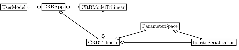
In this section we briefly introduce the organization of the RB framework of _Feel++ (see figure2), and then we see how the user deals with the FE model, needed to interface with the RB framework.

4.3.1. Reduced basis framework

(12)

CRBApp

UserModel CRBModelTrilinear

CRBTrilinear

ParameterSpace

boost::Serialization

Figure 2. Class diagram for theFeel++ RB framework. Arrows represent instantiations of template classes.

As the offline step of the method can be very expensive, scalar products resulting from the projection of matrices or vectors on the RB are saved in a database. To save objects in the database, we use the concept of ”serialization” introduced by the set of libraries for theC++programming languageBoost.

The classCRBAppis the driver for the RB framework. The classParameterSpacemanages the construction of the parameter space. First, if no existing database is found the offline step of RBM is run in order to build a basis, while if a database already exists the basis can be enriched or the algorithm passes to the online step.

To solve a linear or nonlinear problem with RB method in_Feel++the user has to define in his model the variational formulation of the problem. At the state of the art, the variation form must be defined in accord with the affine decomposition, future revisions of the code will introduce an automated affine decomposition.

Note that using _Feel++ the user model can be as well a 1D, 2D or 3D model. It is important to keep

in mind that to interface with the RB framework the user has to provide only the FE model (i.e.parameter space, geometry, variational formulation), it corresponds toUserModelin figure2whose interface derives from CRBModelTrilinear.

The_Feel++RB framework support parallel architectures using the MPI technology. As in the FE frame-work an automatic mesh partitioning using Gmsh (Chaco/Metis) is computed, while every data associated to the reduced basis (scalars, vectors and dense matrices, parameter space samplings,...) are duplicated on each processor. However note that since the mesh is partitioned according the number of processors, finite element approximations and thus the reduced basis functions are in fact spread on all processors. Currently the basis functions are saved in the RB database with their associated partitioning. If they are required for visualization purposes or reduced basis space enrichment, the same data partition as in the initial computations must be used. Another particular attention must be paid to parameter space sampling generation: we must ensure that all processors hold the same samplings. To this end, there are generated in a sequential way by only one processor and then broadcasted to other processors.

4.3.2. Finite element model

Let us illustrate the implementation of the FE solution strategy for the problem (1) using_Feel++, we give the main ideas of the solver function, with the continuation algorithm described above, and the computation of Newton method terms.

In listing 1, we display a snippet of code showing the code describing for a given µ, the solution process to retrieve (u(µ), p(µ), T(µ)): (i)compute the coefficients of the affine decomposition; (ii) assemble the linear terms; (iii)solve the non linear problem where updateJacobianandupdateResidualare computing the jaco-bian and residual respectively during the Newton iterations. Note thatupdateJacobianneed not be called at every iterations. Moreover the code is seamless with respect to geometrical dimension (2D or 3D) and parallel computing.

(13)

{

this- > c o m p u t e T h e t a Q ( mu ); // U p d a t e θ c o e f f i c i e n t s

this- > u p d a t e ( mu ); // U p d a t e a f f i n e d e c o m p o s i t i o n of the l i n e a r t e r m s // n o n l i n e a r i t e r a t i v e solver , s o l v e for U =(u, p, T)

b a c k e n d () - > n l S o l v e ( _ j a c o b i a n = u p d a t e J a c o b i a n , _ r e s i d u a l = u p d a t e R e s i d u a l ,

_ s o l u t i o n= U ); }

As mentioned earlier, at each Newton iteration, the Jacobian matrix and the residual vector are updated. We start with the linear terms which can be precomputed, see section3.2. We show, as an example, the Jacobian sub-matrices assembly. The vectorthetaAq[q]represents the coefficientsθJ defined in (34), while the matrices

Aq[0],Aq[1],Aq[2]are respectively the matricesJ1_,_J2_and_J3_{defined in (}₃₅_{). The assembly of those matrices} is displayed in listing2.

Listing 2. Jacobian Linear terms assembly

// D e f i n i t i o n of m e s h and FE s p a c e Xh = Vh×Qh×Ξh

m e s h _ p t r t y p e m e s h ;

// N p o l y n o m i a l o r d e r

Vh = Pch <N+1 , V e c t o r i a l >( m e s h ); Qh = Pch <N>( m e s h );

Xih = Pch <N+1 >( m e s h ); Xh = Vh * Qh * Xix ;

// D e f i n i t i o n of f u n c t i o n s

e l e m e n t _ t y p e U ( Xh , " u " ); e l e m e n t _ t y p e V ( Xh , " v " );

// V e l o c i t y f u n c t i o n and t e s t f u n c t i o n

e l e m e n t _ 0 _ t y p e u = U . element <0 >(); e l e m e n t _ 0 _ t y p e v = V . element <0 >();

// P r e s s i o n f u n c t i o n and t e s t f u n c t i o n

e l e m e n t _ 1 _ t y p e p = U . element <1 >(); e l e m e n t _ 1 _ t y p e q = V . element <1 >();

// T e m p e r a t u r e f u n c t i o n and t e s t f u n c t i o n

e l e m e n t _ 2 _ t y p e t = U . element <2 >(); e l e m e n t _ 2 _ t y p e s = V . element <2 >();

// 1) F l u i d e q u a t i o n s

// 1 . 1 ) V e l o c i t y d i f f u s i o n : Aq [0] = C = R_Ω∇u:∇v

f o r m 2(_ t e s t= Xh ,_ t r i a l= Xh ,_ m a t r i x= Aq [0] ) =

i n t e g r a t e( _ r a n g e =e l e m e n t s( m e s h ) , _ e x p r =t r a c e(g r a d t( u )*t r a n s(g r a d( v ))) );

// 1 . 2 ) H e a t d i f f u s i o n : Aq [1] = G = R_Ω∇t· ∇s

f o r m 2( _ t e s t= Xh ,_ t r i a l= Xh ,_ m a t r i x= Aq [1] ) =

i n t e g r a t e( _ r a n g e =e l e m e n t s( m e s h ) , _ e x p r =g r a d t( t )*t r a n s(g r a d( s )) );

// 1 . 3 ) P r e s s u r e - v e l o c i t y t e r m s : Aq [2] = - B = R_Ω−p ∇ ·v

f o r m 2( _ t e s t= Xh ,_ t r i a l= Xh ,_ m a t r i x= Aq [2] ) =

i n t e g r a t e ( _ r a n g e =e l e m e n t s( m e s h ) , _ e x p r = - idt( p ) * div( v ) );

// Aq [2] += B ^ t = R_Ωq ∇ ·u

f o r m 2( _ t e s t= Xh ,_ t r i a l= Xh ,_ m a t r i x= Aq [2] ) +=

i n t e g r a t e ( _ r a n g e =e l e m e n t s( m e s h ) , _ e x p r =d i v t( u ) * id( q ) );

// 2) T e m p e r a t u r e e q u a t i o n

// 2 . 1 ) B u y o a n c y f o r c e s : Aq [2] += D = R_Ωt e2 v

i n t e g r a t e( e l e m e n t s( m e s h ) , -idt( t )*( t r a n s( vec ( cst (0.) , cst ( 1 . 0 ) ) ) *id( v ) ) );

// B . C . ...

form2(Xh,Xh,M)builds a bilinear formXh×Xh→Rwhose algebraic contribution will be stored in the matrix

(14)

element space of degree 3 for vectorial functions (velocity),Qhis a scalar function space of degree 2 (pression) and Xiha scalar space of degree 3 (temperature). Again this is seamless for the user with respect to parallel computing and quite expressive with respect to the mathematical formulation.

Finally we add the contribution of the non-linear terms to the jacobian. The main operations required to this update are showed in listing3. We remark that for a givenµthe linear part of the jacobian stored inJlin does not need to be updated, its implementation is computed once for all using the code displayed in listing2.

Listing 3. Non-linear terms assembly in jacobian

v o i d C o n v e c t i o n :: u p d a t e J a c o b i a n ( c o n s t v e c t o r _ p t r t y p e & X , s p a r s e _ m a t r i x _ p t r t y p e & J ) {

// D e f i n i t i o n of m e s h and FE s p a c e Xh , and d e f i n i t i o n of f u n c t i o n s // are d o n e in the s a m e way as p r e v i o u s l y

Aq [3][0] - > z e r o (); // i n i t i a l i z a t i o n

// 1) F l u i d e q u a t i o n s - f l u i d c o n v e c t i o n d e r i v a t i v e s : // Aq [3] = u ^ T * A + A * u = R_Ω(u ∇ ·vi vj+vi ∇ ·u vj)

i n t e g r a t e ( _ r a n g e =e l e m e n t s( m e s h ) , t r a n s( id( v ) )*( g r a d v( u ) )*idt( u ) );

i n t e g r a t e ( _ r a n g e =e l e m e n t s( m e s h ) , t r a n s( id( v ) )*( g r a d t( u ) )*idv( u ) );

// 2) T e m p e r a t u r e e q u a t i o n - h e a t c o n v e c t i o n : // Aq [3] += u ^ T * E + E * T = R_Ω(u· ∇(si)sj+ui· ∇(T)sj)

i n t e g r a t e ( e l e m e n t s( m e s h ) , g r a d( s )*( idv( t )*idt( u ) ) );

i n t e g r a t e ( e l e m e n t s( m e s h ) , g r a d( s )*( idt( t )*idv( u ) ) );

// B . C . ...

// J a c o b i a n = l i n e a r t e r m s of A f f i n e D e c o m p o s i t i o n + N o n l i n e a r t e r m Aq [3]

J - > z e r o (); J - > a d d M a t r i x (1. , J l i n ); J - > a d d M a t r i x (1. , Aq [ 3 ] ) ; }

5. Numerical Experiments

We present some numerical results: first we compare flow profiles obtained using FEM and RBM, and

associated errors, in both 2D and 3D cases. Then, computational times and performances varying model

parameters are show in both FEM and CRB cases are displayed. Finally, we compare the average temperature obtained in both cases.

Thanks to the _Feel++ framework, the finite element and reduced basis models are available both in 2D

and 3D.

(15)

is run on 24 processors. In the 2D case we use the solver GMRES and the Additive Schwarz Method (GASM) as preconditioner, whereas the preconditioner LU is used in the 3D case.

5.1. Flow profiles

First we look at the solutions obtained with RBM and compare them with the FEM ones. We investigate the relative error between the two resolutions for increased turbulent flow,i.e.high parameters.

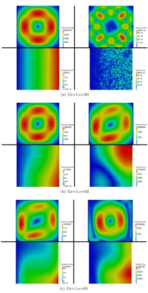
Figure 3 shows 2D results for different Grashof values (1, 103_{, 10}5_{). On the left there are RBM solutions,} we show the velocity magnitude (top) and temperature (bottom) profiles. We observe faster flow for increased Grashof values as expected. On the right, relative errors for velocity (top) and temperature (bottom) are shown. As the flow is more turbulent for increasing parameters, the relative errors increase as well. Furthermore, errors is at least 2×10−3 _{for velocity magnitude and 10}−2 _{for temperature profile, which are satisfactory values (we} do not consider values forGr = 1 because of it corresponds to a parameter used to build the basis, the error is as expected 10−16_).

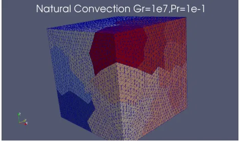
We analyze the error in 2D and 3D simulations, respectively Figures5(c)and6(c), increasing Grashof values. We observe in both cases that the error increases for Grashof between 1 and 103 _{and it stabilizes for values} greater than 103_{. Also, we remark that the solution in a finite 3D tank for high Grashof value represents a flow} with a complex pattern (Figure4).

5.2. Performances

We now compare the RBM computational gain with respect to FEM. Figures5(b)and 6(b)show the

com-putational times for increased Grashof in both FEM and RBM cases, respectively in the 2D and 3D tanks. In both cases, we show the log-log plot of the computational times (in seconds) vsGr.

As expected the FEM solution costs is several order more expensive than the RBM one. In particular, we have a factor 6×102 _{for small Grashof and we reach a factor 1}_.₅_×₁₀3 _{for high Grashof in 2D case, and a} factor from 103 _{to 10}4 _{occurs in 3D case. Furthermore, we observe that the computational time increases in} parameters in the case of FEM, while it is almost constant in RBM computations. In both 2D and 3D cases we find few parameters that lead to a higher computational time in RB, this is due to increased number of online Newton iterations, however it still yield good results when inspecting the average temperature, see Figure5(a) and Figure6(a).

In figures 5(b) and6(b), the computational time comparison between FEM and RBM does not include the offline step of the RBM.

version1 :

The offline step’s time depends on the choice of the basis and we can suppose that an efficient basis can be built once for all and used to solve several reduced problems. Anyhow, in the case we deal with, the offline step take a long time (more details on the basis construction are given at the beginning of this section). For instance, in the 2D case, the offline step takes 1.6×103 _{seconds for 28 elements in the reduced basis. Then, if we deal} with a low value of Grashof number — for exampleGr= 1 — the RB computational cost including the offline step will be damped after approximately 200 RB simulations, while for higher Grashof number — for example Gr= 106 _{— the offline-online computational cost is comparable with around 50 RB simulations.}

version2 :

This step can take a long time. For example, in the 2D case, the offline step takes 1 635 seconds for 28 elements in the reduced basis. Then it is legitimate to wonder how many runs are needed so the RBM becomes interesting. Of course it depends on the value of parameters. For a low Grashof ( say 1 ) then 190 runs are necessary before the RBM becomes interesting, whereas for a high Grashof ( say 106 ) only 45 runs are necessary. In the 3D case, the offline step takes 1 940 seconds also with 28 elements in the reduced basis. For a low Grashof 175 runs are necessary before the RBM becomes interesting, whereas it is only 30 for a high Grashof.

(16)

(a) Gr=1.e+00

(b) Gr=1.e+03

(c) Gr=1.e+05

(17)

(a) mesh partitioning (24 processors)

(b) temperature isosurfaces (c) Stream lines

Figure 4. 3D computations forGr= 1e7, P r= 0.1

than the dimensionN of the RB space since we need to take into account the cost of the reduction computation are not marginal, it scales asN3_{due to the non-linear terms.}

We remark that we do not apply the continuation algorithm neither for FEM nor for RBM. However it may become necessary for FEM resolution in case of non-convergence of the Newton solver, for higher parameter values or more complex geometry. As initial guess of the Newton Algorithm used to solve the online RB problems, the nearest known solution is used, whereas in FEM the initial guess is taken as the zero — although we could also use the nearest basis function as initial guess.

5.3. Outputs

To conclude we look at the average temperature on boundary Γ3 = ¯Ω∩ {x= 1} (see Figure 1 for the 2D tank)

Tav=

Z

Γ3

T dσ. (43)

(18)

100 ₁₀1 ₁₀2 ₁₀3 ₁₀4 ₁₀5 ₁₀6

10−0.8

10−0.6

10−0.4

10−0.2

100 Gr Ta v FEM RB

(a)TavversusGr

100 ₁₀1 ₁₀2 ₁₀3 ₁₀4 ₁₀5 ₁₀6

10−2

10−1

100 101 Gr Computational time (s) FEM RB

(b) Computational time versusGr

100 ₁₀1 ₁₀2 ₁₀3 ₁₀4 ₁₀5 ₁₀6

10−6

10−5

10−4

10−3

10−2

10−1

Gr R el ativ e er r or

|sN(µ)−sN(µ)| |sN(µ)|

(c) Error versusGr

Figure 5. 2D computations forGr∈[1; 1e6],P r= 1.

101 ₁₀2 ₁₀3 ₁₀4 ₁₀5 ₁₀6

10−0.6

10−0.4

10−0.2

100

Gr Tav

FEM RB

(a)TavversusGr

101 ₁₀2 ₁₀3 ₁₀4 ₁₀5 ₁₀6

10−2

10−1

100 101 102 Gr Computational time (s) FEM RB

(b) Computational time versusGr

101 ₁₀2 ₁₀3 ₁₀4 ₁₀5 ₁₀6

10−6

10−5

10−4

10−3

10−2

Gr R el ativ e er r or

|sN(µ)−sN(µ)| |sN(µ)|

(c) Error versusGr

Figure 6. 3D computations forGr∈[1; 1e6],P r= 1.

6. Conclusions and perspectives

We have presented a mathematical and computational treatment of the RBM applied to steady-state natural convection. This can be readily applied to other types of problems with quadratic non-linearities. The proposed method gives results that are accurate and efficient. In particular, the efficiency of this technique is remarkable in the case of flows with complex patterns both in 2D and 3D. From a framework point of view, the (offline) database handling raises interesting challenges when dealing with large parallel data.

In terms of perspectives, a posteriori error estimation is a first step not only to assess the quality of the RB approximation but also to guide the RB space construction using greedy strategies [VP05,Yan12,VPRP03]. More complex applications can be considered in particular including geometrical parameters. However it is foreseen that we may require hp-RBM approximations, see e.g. [EHKP12]. Finally, we dealt with the steady-state of the natural convection flow, the transient steady-state is also of interest but requires much more involved mathematical and computational framework, seee.g. [Yan12].

Acknowledgements

(19)

References

[ADL00] P.R. Amestoy, I.S. Duff, and J.-Y. L’Excellent. Multifrontal parallel distributed symmetric and unsymmetric solvers.

Computer Methods in Applied Mechanics and Engineering, 184(2-4):501 – 520, 2000.

[BBB+_12a] _{S. Balay, J. Brown, K. Buschelman, V. Eijkhout, W. D. Gropp, D. Kaushik, M. G. Knepley, L. Curfman McInnes,} B. F. Smith, and H. Zhang.PETSc Users Manual, 2012.

[BBB+12b] S. Balay, J. Brown, K. Buschelman, W. D. Gropp, D. Kaushik, M. G. Knepley, L. Curfman McInnes, B. F. Smith, and H. Zhang.PETSc Web page, 2012.

[BGCMS97] S. Balay, W. D. Gropp, L. Curfman McInnes, and B. F. Smith.Efficient Management of Parallelism in Object Oriented Numerical Software Libraries, 1997.

[Cha13] V. Chabannes.Vers la simulation des ´ecoulements sanguins. PhD thesis, Universit´e Joseph Fourier, Grenoble, july 2013.

[DVTP13] C. Daversin, S. Veys, C. Trophime, and C. Prud’Homme. A reduced basis framework: Application to large scale nonlinear multi-physics problems. Submitted to ESAIM proceedings, 2013.

[EHKP12] J.L. Eftang, D.B.P. Huynh, D.J. Knezevic, and A.T. Patera. A two-step certified reduced basis method.Journal of Scientific Computing, 51:28–58, 2012.

[GR09] C. Geuzaine and J.-F. Remacle. Gmsh: a three-dimensional finite element mesh generator with built-in pre-and post-processing facilities, 2009.

[PCD+_12] _{C. Prud’Homme, V. Chabannes, V. Doyeux, M. Ismail, A. Samake, and G. Pena. Feel++: A computational framework} for galerkin methods and advanced numerical methods. InESAIM: PROCEEDINGS, pages 1–10, 2012.

[PP04] C. Prud’homme and A.T. Patera. Reduced-basis output bounds for approximately parameterized elliptic coercive partial differential equations.Computing and Visualization in Science, 6(2-3):147–162, 2004.

[Pru06] C. Prud’homme. A domain specific embedded language in C++ for automatic differentiation, projection, integration and variational formulations. Scientific Programming, 14(2):81-110, 2006.

[PRV+02] C. Prud’homme, D. V. Rovas, K. Veroy, L. Machiels, Y. Maday, A. T. Patera, and G. Turinici. Reliable real-time solution of parametrized partial differential equations: Reduced-basis output bound methods.Journal of Fluids En-gineering, 124(1):70–80, 2002.

[QRM11] A. Quarteroni, G. Rozza, and A. Manzoni. Certified reduced basis approximation for parametrized partial differential equations and applications.Journal of Mathematics in Industry, 1(1):1–49, 2011.

[RHP07] G. Rozza, D.B.P. Huynh, and A.T. Patera. Reduced basis approximation and a posteriori error estimation for affinely parametrized elliptic coercive partial differential equations. Archives of Computational Methods in Engi-neering, 15(3):1–47, 2007.

[SBG04] B. Smith, P. Bjorstad, and W. Gropp.Domain decomposition: parallel multilevel methods for elliptic partial differential equations. Cambridge University Press, 2004.

[VCD+_12] _{S. Veys, R. Chakir, C. Daversin, C. Prud’homme, and C. Trophime. A computational framework for certified} re-duced basis methods: application to a multiphysic problem. InConference Record of the 6th European Congress on Computational Methods in Applied Sciences and Engineering, 2012.

[VDPT12] S. Veys, C. Daversin, C. Prud’homme, and C. Trophime. Reduced order modeling of high magnetic field magnets. In

Conference Record of the 11th International Workshop on Finite Elements for Microwave Engineering, 2012. [VP05] K. Veroy and A.T. Patera. Certified real-time solution of the parametrized steady incompressible navier-stokes

equa-tions: Rigorous reduced-basis a posteriori error bounds.Int. J. Numer. Meth. Fluids, 47:773–788, 2005.

[VPP03] K. Veroy, C. Prud’homme, and A.T. Patera. Reduced-basis approximation of the viscous Burgers equation: Rigorous

a posteriori error bounds.C. R. Acad. Sci. Paris, S´erie I, 337(9):619–624, November 2003.

[VPRP03] K. Veroy, C. Prud’homme, D. V. Rovas, and A.T. Patera.A posteriorierror bounds for reduced-basis approximation of parametrized noncoercive and nonlinear elliptic partial differential equations (AIAA Paper 2003-3847). InProceedings of the 16th AIAA Computational Fluid Dynamics Conference, June 2003.