Improving System Reliability Assessment of Safety-Critical Systems using Machine Learning Optimization Techniques

www.astesj.com

Special issue on Advancement in Engineering Technology

ISSN: 2415-6698

Improving System Reliability Assessment of Safety-Critical

Systems using Machine Learning Optimization Techniques

Ibrahim Alag¨oz*1_{, Thomas Hoiss}2_{, Reinhard German}1

1_{Department of Computer Science 7, FAU Erlangen-Nuremberg, 91058, Germany} 2_{Automotive Safety Technologies GmbH, 85080, Gaimersheim, Germany}

A R T I C L E I N F O A B S T R A C T

Article history:

Received: 14 November, 2017 Accepted: 10 January, 2018 Online: 30 January, 2018 Keywords:

Safety-Critical System Black Box Regression Testing Linear Classifier

Selection Prioritization

Quality assurance of modern-day safety-critical systems is continually facing new challenges with the increase in both the level of functionality they provide and their degree of interaction with their environment. We propose a novel selection method for black-box regression testing on the basis of machine learning techniques for increasing testing efficiency. Risk-aware selection decisions are performed on the basis of reliabil-ity estimations calculated during an online training session. In this way, significant reductions in testing time can be achieved in industrial projects without uncontrolled reduction in the quality of the regression test for assessing the actual system reliability.

1

Introduction

Reliability assessment of safety-critical systems is be-coming an almost insurmountable challenge. In the near future, the engineering of new applications for vehicles such as driving assistance functions or even autonomous driving systems will inevitably incur sig-nificantly increased engineering sophistication and longer test cycles. Thus, in the automotive domain, functional safety continues to be ensured on the ba-sis of the international ISO 26262 standard. As both the levels of functionality such systems provide and their degree of interaction with their environment in-creases, an adequate increase in system safety assess-ment capabilities is required.

This paper is an extension of work originally pre-sented at the 10th IEEE International Conference on Software Testing, Verification and Validation (ICST 2017) [1] and describes a methodology for efficiently assessing system safety. The focus of the paper is on regression testing of safety-critical systems consisting of black-box components. This scenario is common for automotive electronic systems, where testing time is expensive and should be reduced without an uncon-trolled reduction in reliability.

The work reported here correspondingly seeks to increase testing efficiency by reducing the number of selected test cases in a regression test cycle. When a

selection decision is made, the following two types of errors are possible:

• a test case is selected but would pass (type-I-error, false-positive case) and

• a test case is not selected but would fail (type-II-error, false-negative case).

Accordingly, we model a classifier ˆH for solving the following optimization problem.

minpFP =P( ˆH=H1|H0)

subject topFN=P( ˆH=H0|H1)≤pFN ,MAX

(1)

A good standard of test efficiency calls for the avoidance of false-positives. This requires minimiza-tion of the probability of mistakenly assuming the ri-val hypothesis (H1 : test case fails) even though the null hypothesis (H0: test case passes) is correct. Con-versely, false-negatives mean that system failures re-main undetected; the occurrence of this type of error must therefore be avoided with very stringent require-ments. Thus, a predefined limitpFN ,MAX for the

prob-ability of a false-negative is defined.

[1] proposed a concept for the selection of test cases based on a stochastic model. However, this pa-per proposes a holistic optimization framework for the safety assessment of safety-critical systems based on machine learning optimization techniques. We

*_{Corresponding Author: Ibrahim Alag¨oz, Hornstr. 1 85051 Ingolstadt, [email protected]}

suggest an incrementally and actively learning linear classifier whose parameters are estimated on the ba-sis of Bayesian inference rules. As a result, our novel approach for modeling a linear classifier outperforms other machine learning approaches in terms of sensi-tivity.

Furthermore, this paper deals with the following fundamentally important research question: The ma-chine learning approach is trained with data (test evaluations) obtained during a concurrently running regression test. How much training data is enough? When does regression test selection actually start?

We extend the proposed selection method [1] by introducing suitable test case features that are used in the machine learning approach for increasing perfor-mance (see [2]). Therefore, each feature introduced increases the complexity of the optimization problem (cf. Eq. 1) as a new dimension for optimization is introduced. Thus [3] and [4] suggest that high dimen-sional optimization problems can be solved in reason-able timeframes by using evolutionary algorithms in-stead of a (grid)search-based approach as given in [1]. Accordingly, we propose an evolutionary optimiza-tion approach for increasing testing efficiency.

Further extensions, such as the introduction of a prioritization strategy for test cases in order to se-lect higher-priority test cases, will also be presented within this paper. In our novel approach, a linear clas-sifier is trained in an online session; the ordering of the training data on the basis of a prioritization strat-egy therefore has the potential to improve our classi-fiers’ performance.

We also provide an industrial case study to show the advantages of the suggested selection method. The study uses data from several regression test cycles of an ECU of a German car manufacturer, showing how test effort can be reduced significantly whereas the rates of both false-negatives and false-positives can be kept at very low values. In this example, we can quadruple test efficiency by keeping the false-negative probability at 1%.

We first discuss related work in Sec. 2 and explain basic definitions in Sec. 3. Accordingly, we motivate our research topic in Sec. 4 by giving some back-ground information on regression tests and referring to the challenges. In Sec. 5, we give a brief overview of known machine learning methods’ performance in solving safety-critical binary classification tasks. The concept of our novel machine learning approach is presented in Sec. 6. Sec. 7 discusses optimization strategies, and Sec. 8 focuses on the importance of the learning phase for the success of our approach. An in-dustrial case study with real data is then given in Sec. 9. Finally, Sec. 10 presents the paper’s conclusions.

2

Related Work

The automotive industry is currently engaged in a la-borious quality assessment process around new engi-neered driver assistance and active and passive safety

functions, while functional safety is ensured accord-ing to the international ISO 26262 standard [5]. Re-liability assessment of systems is therefore, possible through both model-checking and testing.

Model-checking is used for verifying conditions on system properties. Thus [6] states that system require-ments can also be validated by model-checking tech-niques. The idea is to check the degree to which sys-tem properties are met and to deduce logical conclu-sions on the basis of the satisfaction of system require-ments. Model-checking has therefore gained wide ac-ceptance in the field of hardware and protocol veri-fication communities [7]. Motivated by the fact that numerical model-checking approaches cannot be di-rectly applied to black-box components as a usable formal model is not available, we focus on model-checking driven black-box testing [6] and statistical model-checking techniques [8]. However, there ex-ist some approaches for interactively learning finite state systems of black-box components (see [9] and [10]), which are proposed asblack box checkingin [11]. Learning a model is an expensive task, as the interac-tively learned model has to be adapted due to inaccu-racy reasons. Nevertheless, some assumptions about the system to be checked, such as the number of inter-nal states, are necessary; furthermore, conformance testing for ensuring the accuracy of the learned model has to be iteratively performed [9].

Therefore, [8] outlines the advantages of statisti-cal model-checking as being simple, efficient and uni-formly applicable to white- and even to black-box sys-tems. [6] motivates on-the-fly generation of test cases for checking system properties; here, a test case is gen-erated for simulating a system for a finite number of executions. All these executions are used as individ-ual attempts to discharge a statistical hypothesis test and finally for checking the satisfaction of a dedicated system property.

Model-checking driven testing, or even simply testing a system in order to validate its requirements, is an expensive task, especially where safety-critical systems are concerned. However, the focus is on re-gression testing, which means that the entire system under test has already been tested once but has to be tested again due to system modifications that have been carried out. The purpose of regression testing is to provide confidence that unchanged parts within the system are not affected by these modifications [12]. White-box selection techniques have been com-prehensively researched [13, 14]. However, we are here considering black-box components, and hence selecting test cases that only check modified system blocks gets difficult.

Since the implementation of black-box systems and moreover, the information on performed system modifications is not available [12], reasonably con-ducting a regression test becomes impossible.

Accordingly, regression testing of safety-critical black-box systems ends up in simply executing all ex-isting test cases; this is aretest-allapproach [12].

au-tomotive industry, up to 80% of system failures [1] that are detected during a regression test have not oc-curred previously. The reason behind this fact is that often many unintended bugs are introduced during a bug-fixing process. So between two system releases many new unknown errors are often introduced.

For reducing the overall test effort, we apply a test case selection method [1] based on hypothesis tests. Those test cases that are assumed to fail on their exe-cutions are accordingly selected. However, type errors while performing hypothesis tests are possible, as, for instance, in statistical model-checking.

We extend the proposed selection method into a holistic machine learning-driven optimization frame-work that utilizes suitable test case features for in-creasing testing efficiency (see [2]). Machine learning methods are often trained in so-calledbatch modes. Nevertheless, many applications in the field of au-tonomous robotics or driving are trained on the ba-sis of continuously arriving training data [15]. Thus, incremental learning facilitates learning from stream-ing data and hence is exposed to continuous model adaptation [15]. Especially handling non-stationary data assumes key importance in applications like voice and face recognition due to dynamically evolv-ing patterns. Accordevolv-ingly, many adaptive clusterevolv-ing models have been proposed, including incremental K-means and evolutionary spectral clustering tech-niques [16].

Furthermore, labeling input data is often awkward and expensive [17] and hence accurately training models can be difficult. Therefore, semi-supervised learning techniques are developed for learning from both labeled and unlabeled data [17]. Motivated by these techniques, we propose a similar approach for effectively learning from labeled data. Hence, we clus-ter binary labeled data in more than two clusclus-ters for improving a classifier’s learning capability due to the optimization of an objective function. Our tion framework thus utilizes evolutionary optimiza-tion algorithms for handling the optimizaoptimiza-tion com-plexity. Minimization of labeling cost on the basis of active learning strategies [18, 19] will also be dealt with in this paper.

3

Basic Definitions

We define the test suiteT ={_ti |₁≤_i≤_M}_consisting of a total ofMtest cases. TExec∈T andTExec∈T are

subsets ofT that contain test cases that are executed and deselected in a current regression test respec-tively. Based on the test case executions (∀_ti ∈_TExec), a system’s reliability is actually learned, and thus the machine learning algorithm is trained.

The focus in supervised learning is on understand-ing the relationship between feature and data (here test case evaluation) [4]. Therefore, a test case needs to code a feature vector so that the indication of the coded features for a system failure can be learned in a supervised fashion. Such an indication is not just

a highly probable forecast of an expected system fail-ure, it is rather a particular risk-associated recogni-tion.

First of all, a feature can be any individual measur-able property of a test case. The data type of a feature is mostly numeric, but strings are also possible. How-ever, such features need to be informative, discrimi-native and independent of one another if they are to be relevant and non-redundant The definition of suit-able features increases the classifier performance [20]. In our application, a feature can be varied, such as a

• subjective ranking of a test case based on expert knowledge. Such rankings can hint at the error susceptibility of verified parts of the system;

• verified function’s safety integrity level, known as theASILin automotive applications [5]; • name of a function whose reliability is assured;

• reference to any hardware component of a cir-cuit board that is being tested in a hardware-in-the-loop (HiL) test environment;

• number of totally involved electronic control units during the testing of a networked func-tionality; Such a number can hint at the com-plexity of the networked functionality and hence at its error susceptibility.

We define the entire set of featuresΦ ={_φf |₁≤

f ≤ _F} _{of test cases that might be relevant for} un-derstanding the behavior of test cases. Thus, features may be e.g. φ1 ={0QM0,0A0,0B0,0C0,0D0}(ASIL) orφ2 ={_f1,f2,f3}_{(function name). Hence, a test case can} verify a functionf3that has anASILA.

The following passages discuss the selection of suitable features, which is an important strategy for improving a classifier’s performance.

• Sometimes less is more - If the defined setΦ is too large it can cause huge training effort, high dimensionality of the optimization problem and overfitting. Thus we define a selection mask

bs=

h

1 0 0· · ·₁i_{of lengthF for selecting} rel-evant features Φ_s. If thef −_{thmatrix entry of} bs is greater than or equal to 1, then the

corre-sponding featureφf ∈Φ is selected and added

toΦs, otherwise not.

• The set of main featuresΦm⊆Φsis coded as

fol-lows: If thef −_{thmatrix entry ofbs is equal to} 2, then the corresponding featureφf ∈Φs is at

the same time a main feature φf ∈ Φm,

other-wise not. The main features are used to estab-lish the overall training data set: The training data is adapted to each test case, and thus it is

Tti ={tj |tj ∈TExec∧ti Φ_m

≡ _tj}_{. Hence, we define} that two test casesti andtjare equivalentti

Φ_s \_Φm,1 ≤ _h ≤ _{H =} |_Φs \_Φm| _{consisting of} fea-turesψl that represent individual combinational

set-tings for features φf ∈ Φs \Φm. In simple terms,

the cross-product of our sample features isφ1×φ2= {₍0_QM0_{, f1),(}0_QM0_{, f2),(}0_QM0_{, f3),(}0_A0_{, f1), ...}} _{Finally, a} Boolean functioncheck:T×_Ψ →Bwithcheck(t_i, ψ_l) =

(

0, ifti’s features are given byψl

1, otherwise

)

is defined.

In addition, the function state:T ×_R→ _{S is} de-fined; it returns the state of a dedicated test case in a concrete regression test. The state has to be either ’Pass’ or ’Fail’, except for cases where the test case has not been executed so that its state is undefined. There-fore, S ={_{’Pass’,’Fail’,’Undefined’}}_{defines the set of} possible states. Furthermore, the setR={_rk |₀≤_k≤

K}_{includesr0which is the current regression test and} older regression tests starting from the last regression

r1to the first considered regressionrK. Lastly, we

de-fine the tuplehistory(ti) ={state(ti, r1), ..., state(ti, rK)}

containingti’s previous test results.

4

Motivation

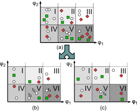
In practice, finding suitable features is a difficult task. Since we focus here on black-box systems, system-internal information is not available that might be useful for understanding the system behavior. As a reason, we can only define the above listed features, which might be too high-level for classifying system failures. To illustrate this fact, Fig. 1 a) shows a typical situation: The behavior of test cases in relation to arbi-trarily defined featuresφ1andφ2is given. Passed and failed test cases are presented by green squares and red diamonds respectively, and white circles stand for test cases yet to be executed.

I

II

III

IV

V

VI

t1

t2

t3 t4

φ1

φ2

φ1

φ2 φ2

φ1 φ1

I

II

III

IV

V

VI

I

II

III

IV

V

VI

(a)

(b) (c)

Figure 1: An artificial regression test with test cases.

We can see that the green squares and the red di-amonds are widely scattered. Thus, defining a hyper-plane in order to set two acceptance regions for pass-ing and failpass-ing test cases is no easy matter. In order to solve this complex task, we develop a novel approach

that is basically motivated by the following thought experiment: All test cases that are represented in Fig. 1 a) are now either assigned to 1 b) or 1 c) accord-ing to a certain mappaccord-ing. The individual mappaccord-ings of test cases will be discussed later, in Sec. 6. In the next step, a cross-product transformation is performed in order to group test cases into sub-regions (we refer these later as sub-clusters). In our example, we cre-ate six sub-regions. Table 1 lists the empirical failure probabilities of each sub-region.

In order to keep our thought experiment very sim-ple, we will neglect statistical computations for now and focus only on the main idea of our novel ap-proach. The introduction of Bayesian networks and hence the derivation of weights for linear classifiers will be discussed later, in Sec. 6. We assume for now that the calculated failure probabilities of test cases in Fig. 1 b) and Fig. 1 c) are correlated. So our ex-ample remains very simple, we also require that the failure probabilities of the corresponding sub-regions are equal. This assumption reduces the complexity of the following classification task enormously. We will classify the following test casest1,t2,t3andt4 in ac-cordance with whether a selection is necessary or not.

Table 1: Failure probability of each sub-region.

P(H1) I II III IV V VI

Fig. 1 a) 0 0.5 1 1 1/3 3/5

Fig. 1 b) 0 0.5 1 1 0 2/3

Fig. 1 c) 0 0.5 1 1 0.5 0.5

Only ift1passes will the failure probability of sub-region VI in Fig. 1 b) be equal to the failure probabil-ity of sub-region VI in Fig. 1 c). According to this fact,t1is assumed to pass, and hence it is deselected. Furthermore,t2will be selected as a fail of a test case inside sub-region V is expected. However,t2 passes, and, based on the same consideration, t3 is also se-lected and finally fails. Since now a failure probabil-ity of 1/3 is expected in sub-region V, t4 is assumed to pass, and therefore it does not need to be selected. Table 2 summarizes all decisions executed.

Table 2: Test case states and algorithm decisions.

Test Case State Decision Type of Decision

t1 Pass Deselected True-Negative

t2 Pass Selected False-Positive

t3 Fail Selected True-Positive

t4 Pass Deselected True-Negative

precisely estimated on the basis of the calculated cor-relations. In practice, the failure probabilities of same sub-regions in Fig. 1 b) and Fig. 1 c) is often not exactly equal, but these failure probabilities are cor-related. So the main task is to findgood sub-regions for maximizing the empirically evaluated correlations and thus for precisely estimating the behavior of test cases. A more detailed explanation of our novel ap-proach will follow in Sec. 6.

5

Performance of Known Machine

Learning Methods

We have already indicated, by showing the example regression test in Sec. 4 (see Fig. 1), that accord-ing to the distribution of the input data, many ma-chine learning methods cannot be reasonably applied for solving the constrained optimization problem (cf. Eq. 1). We will now demonstrate briefly that train-ing linear classifiers in the classical sense by minimiz-ing a loss function cannot perform well for solvminimiz-ing safety-critical binary classification tasks. The situa-tion is that only a small percentage of the data is ac-tually labeled with one (’Fail’). Furthermore, failed and passed test cases are widely scattered in the fea-ture space, which means detecting failing test cases becomes impossible. Additionally, the performance of deep neuronal networks is validated in the following.

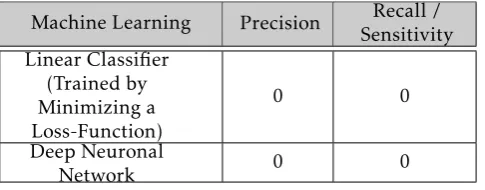
The evaluation results (precision/recall) of these machine learning methods are given in Table 3. Each machine learning method is trained in thebatchmode. The training data consists of all obtained test eval-uations of a special regression test that will also be analyzed in our industrial case study in Sec. 9. For evaluating the machine learning methods, we used the training data first for training and later for test-ing (traintest-ing data = test data). Even so, the sensitivity of both machine learning methods is zero, and thus we propose a novel approach for determining a linear classifier’s parameters in Sec. 6.

Table 3: Performance of known machine learning methods in solving safety-critical binary classification tasks.

Machine Learning Precision Recall /

Sensitivity Linear Classifier

(Trained by Minimizing a Loss-Function)

0 0

Deep Neuronal

Network 0 0

6

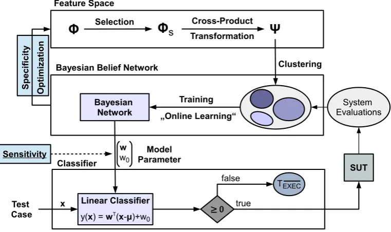
Concept

The concept of our novel approach is shown in Fig. 2. We start with specifying a feature setΦ, and taking its subsetΦ_s and finally constitute a cross-product fea-ture transformation to obtain the setΨ. Based onΨ

and by applying thecheck-function onTExec, test cases

can be grouped. If we look back to the example where we grouped test cases in Fig. 1 a), then we will see that there is a relationship between test cases’ features and their assignments to sub-regions.

Correspondingly, we introduce the definitions of clusters and sub-clusters of test cases. In the first step, test cases∀_tk ∈ _Tt

i are assigned to clusters based on

their history-tuples. A cluster is basically a partition of Tti and consists of test cases that have the same

history-tuples. Accordingly, the number of distinct history-tuplesN determines the total number of clus-ters. This is the step that has already been shown in Sec. 4, where test cases inside Fig. 1 a) were individ-ually mapped into Figs. 1 b) and 1 c). In this way, already executed test cases depicted in Fig. 1 b) be-long to one cluster and, analogously, those executed test cases that are depicted in Fig. 1 c) belong to an-other cluster.

In the next step, each clusterCnis subdivided into

Lsub-clusters. A test casetk ∈Cnis an element of the

l-th sub-clusterCn,l if check(tk, ψl) is true. We

orig-inally introduced the terminology of sub-regions in Sec. 4. However, we focus in what follows on dis-crete valued features, which means that grouping test cases into sub-clusters is more appropriate. By intro-ducing the functioneval:TExec→ {0,1}that is defined

as follows

eval(ti) =

(

0, forstate{_ti,r0}_{= ’Pass’ (2)} 1, forstate{_ti,r0}_{= ’Fail’ (3)}

the calculation of failure probabilities can be given in Eq. 4.

pn,l=

1 |_Cn,l|

X

∀_ti∈_Cn,l

eval(ti) ₍₄₎

The given selection decisions in our example in Sec. 4 (cf. Fig. 1) were taken based on calculated fail-ure probabilities. Additionally, the correlations be-tween the failure probabilities were considered. Ac-cordingly, we need a stochastic model for estimating the classifier’s sensitivity and specificity. We propose a univariate and also a multivariate stochastic model. The short-comings of the univariate stochastic model for solving the optimization problem (cf. Eq. 1) will be discussed later to motivate the introduction of a multivariate stochastic model. First of all, the next step introduces a multidimensional Gaussian distri-bution that constitutes a distridistri-bution for the failure probabilities of test cases. Based on this distribu-tion, two distinct Bayesian Belief networks for both stochastic models will be introduced.

In the following, we interpret pn,l,1 ≤ l ≤ L as

realizations of a random variable Xn. Xn is

Ψ

Feature Space

Bayesian Belief Network

System Evaluations

Bayesian Network

S

p

e

c

if

ic

it

y

O

p

ti

m

iz

a

ti

o

n

Linear Classifier

y(x) = wT_(x-μ)+w 0

x Test Case

Model Parameter Classifier

w

w₀

Sensitivity

≥ 0

T_EXEC

true false

SUT Selection Cross-Product

Transformation

Training

Clustering

„Online Learning“

Φ

Φ

Figure 2: Determining the weights of a linear classifier for maximizing its specificity under the constraint of a specific sensitivity.

Since each test case evaluation is a binary experi-ment with two possible outcomes (’0’ or ’1’), it can be regarded as a realization of a binary random vari-able. As the sum of independent random variables results into a Gaussian random variable according to the central-limit theorem [21], considering test case evaluations as independent random experiments jus-tifiesXn’s assumed distribution. However, test cases

are executed on the same system and there may be some dependencies between test case evaluations that cannot be directly validated by such means as per-forming code inspections. As a result, we assume a mix of dependent and independent test case eval-uations, and hence the Gaussian assumption is still valid. The moments ofXnareE[Xn] =µn=1L

PL

l=1pn,l

andE[(Xn−E[Xn])2] =σn2=L1−₁

PL

l=1(pn,l−E[Xn])2. As

we introduced in totalN Gaussian random variables, the moments of the multidimensional Gaussian dis-tribution areµ=E[X] = [E[X1], E[X2], ..., E[XN]]T and

Σ=E[(X−_µ)(X−_µ)T_].

Since the constraint of the optimization problem (cf. Eq. 1) has to be fulfilled, an accurate sensitivity estimation has to be iteratively performed.

6.1

Sensitivity Estimation

The formula for calculating the classifier’s false-negative selection probability is given in Eq. 5.

pFN=

NFN

NFN+NT P

≤_{pFN ,MAX (5)}

However, ˆpFN =

ˆ

NFN

ˆ

NFN+NT P has to be estimated, since

the number of mistakenly deselected failing test cases

NFNis unknown, and thus it is estimated by ˆNFN. The

number of already detected failing test cases is given by NT P. Before a decision can be taken on whether

a test caseti can be deselected, the currently allowed

risk of taking a wrong decision has to be estimated in advance. The estimation of ˆNFNhas to be adjusted by

the termxP( ˆH=H0|H1), wherexis the failure prob-ability ofti andP( ˆH =H0|H1) is the estimated false-negative probability if ti is deselected. Accordingly,

the recursive formulation ˆNFN ,new= ˆNFN ,old+xP( ˆH=

H0|H1) is continuously updated whenever an arbi-trary test case is deselected. As ˆpFN ≤pFN ,MAX ⇔

ˆ

NFN ,new

ˆ

NFN ,new+NT P

≤_{pFN ,MAX is required, the maximum} al-lowed false-negative probability for deselecting the next test casetiis given in Eq. 6.

P( ˆH=H0|H1)≤

NT P·pFN ,MAX

1−_{pFN ,MAX} −NˆFN ,old

x

=:pFN ,Limit=:

pFN ,Bound

x

(6)

6.2

Univariate Stochastic Model

We model the Bayesian Network that consists of the random variablesX,Hand ˆH, in Fig. 3. In the uni-variate stochastic model, the focus is on modeling of only one failure probability distribution. Thus the random variableXstands for the previously defined

X1 and its realizationxis given byp1,l wherel is the

index of that sub-clusterC1,lthat fulfillsti∈C1,l.

X

H

H

^

Figure 3: Bayesian Network consisting of the random variablesX,Hand ˆH.

test case states and classifier decisions. As the state of a test caseti is a-priori unknown, it needs to be

mod-eled by a corresponding random variable. According to the realization of X, a pass or a fail of the corre-sponding test caseti, whose failure probability

distri-bution is modeled byX, is expected. Finally, ˆH takes a decision forti based on its failure probabilityx:

ˆ

H(x) =

( _H

0, ifx∈ X0= [0;pT H[ (7)

H1, ifx∈ X1= [pT H; 1] (8)

According to ˆH’s selection rule a very simple hyper-plane y(x) =x−_{pT H is derived where in the case of}

y(x) ≥ _{0 a selection decision is taken. A} particu-larly important factor is the definition of the threshold probabilitypT H, as its setting determines the

classi-fier’s sensitivity and specificity. The common ways of estimating false-negative and false-positive probabil-ities are given in equations 9 and 10, respectively.

ˆ

pFN=

Z

X₀

p(X|_{H1)dx (9)}

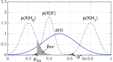
However, we could only estimate the probability den-sity function (pdf)p(X) in contrast to the conditional probability density functions p(X|_{H0) and p(X}|_H1). The reason for this is that pdf estimations are based on mean calculations of test case evaluations. Hence passing and failing test cases are both considered in calculating average failure probabilities. Thus, p(X) is a distribution over failure probabilities of passing as well as failing test cases. Accordingly,p(X|_{H0) and}

p(X|_{H1) cannot be estimated and in conclusion, ˆpFN} and ˆpFP cannot be estimated as in Eq. 9 and 10.

ˆ

pFP =

Z

X₁

p(X|_{H0)dx (10)}

Fig. 4 shows the important probability distribution functions that are used for estimating ˆpFNand ˆpFP.

p(X)

p(X|H 1) p(X|H

0)

p TH

p* TH

Figure 4: Considered probability distribution func-tions in the univariate stochastic model.

The threshold probabilitypT H is calculated based

on the estimation of ˆpFN as the following relation in

Eq. 11 holds.

ˆ

pFN=P(X < p

∗

T H|H1) (11)

As Eq. 11 cannot be directly estimated, the follow-ing relation in Eq. 12 is used for estimatfollow-ing ˆpFN and

finally forpT H.

ˆ

pFN=P(X < pT H|H1)≤P(X < pT H)≤pFN ,Limit (12)

ˆ

pFN is estimated in Eq. 12 according to the

assump-tion that the quantiles ofp(X|_{H1) are larger than the} quantiles of p(X). By solving Eq. 12 the threshold probability is computed as given in Eq. 13

pT H= erfinv(2pFN ,Limit−1)σ

√

2 +µ (13)

with µ =E[X] and σ =pV AR(X). As a result, the classifier’s sensitivity is larger than 1−_{pFN ,Limit, since} its false-negative selection probability is smaller than

pFN ,Limit. Finally, the decision regions of the linear

classifier are defined (cf. Eq. 7 and 8) by determining

pT H.

Furthermore, the minimization of the classifier’s specificity is required by the definition of the con-straint optimization problem (cf. Eq. 1). Accord-ingly, the classifier’s false-positive selection probabil-ity is estimated as given in Eq. 14 and shown in Fig. 4.

ˆ

pFP=P(X≥pT H|H0) (14) However, p(X|_{H0) is not given and thus ˆpFP cannot} reasonably be estimated. Furthermore, ˆpFP cannot be

reasonably minimized as an optimization parameter is not defined; consequently, we need a so-called mul-tivariate stochastic model for performing this. In the first instance, the idea of minimizing ˆpFP and hence

gaining testing efficiency by regarding several distri-bution functions is explained.

6.3

Preliminaries

Let us assume that two dependent Gaussian random variables X andX0

are given. The focus is again on estimating ˆpFN and ˆpFP. Fig. 5 shows the probability

distribution functionsp(X),p(X|_{H0) andp(X}|_{H1) as in} Fig. 4. Additionally, the a-posteriori failure probabil-ity distribution functionp(X|_X0_{) is shown.}

p(x)

p(X|H

1)

p(X|H

0)

p(X|X')

p

TH

p*

TH

Figure 5: Qualitatively minimizing ˆpFP by

introduc-ingp(X|_X0_{) and hence by using conditional} informa-tions.

consid-erably more representative a-posteriori failure proba-bility distribution function that is relatively narrow within a certain range. Sop(X|_X0_{) is considered as the} more representative distribution for the failure proba-bilities and hence ˆpFNandpT Hare estimated by using

this distribution function. Comparing Figs. 4 and 5, it can easily be seen that ˆpFP is basically minimized,

since the risk of a false-negative selection probability is computed based onp(X|_X0_{), which allows a more} representative risk estimation.

All in all, by regarding a set of dependent Gaus-sian random variables and by using the information about their observations, a more representative a-posteriori failure probability distribution function is achieved, which allows a more precise risk estimation. Accordingly, the probability of false-positive selection can be minimized. As a result, a multivariate stochas-tic model is created to exploit the dependency infor-mation between random variables for finally achiev-ing testachiev-ing efficiency.

6.4

Multivariate Stochastic Model

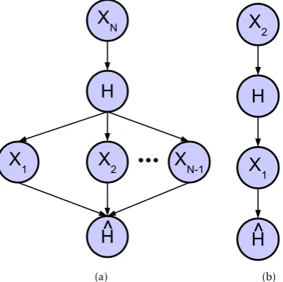
By using the dependency between the random vari-ablesXn,1≤n≤N, a considerably more accurate

es-timation of ˆpFN is achieved and hence ˆpFP is

mini-mized. Fig. 6 shows the modeled Bayesian network consisting of the random variablesXn,1≤n≤N,H

and ˆH.

X

H

H

^

X

X

X

(a)

X

H

H

^

X

(b)

Figure 6: Bayesian Network consisting of an (a) in-definite and (b) in-definite number of random variables

Xn,1≤n≤N.

The focus is on taking a selection decision for an arbitrary test caseti.XNnow models the failure

prob-ability distribution ofti. In our previous example, as

shown in Fig. 1 c), the failure probability distribution of test caset4was calculated based on the empirically evaluated failure probabilities of test cases inside Fig. 1 c). Thust4was an element ofC2(N = 2), and its fail-ure probability was modeled byX2. Analogously,X1

was defined by the empirically evaluated failure prob-abilities of test cases inside Fig. 1 b). In the interest of simplification, we always assume that the currently focused test caseti is an element of cluster CN and

thusXN models its failure probability distribution.

Furthermore, we can calculate the dependency amongXn,1≤n≤N. However, the Bayesian network

in Fig. 6 models the statistical dependency between

H and further random variables Xn,1 ≤ n ≤ N −1.

These dependencies cannot be calculated, but have to be modeled for estimating ˆpFN and ˆpFP.

First of all, we model the classifier ˆH(·_{) as follows}

ˆ

H(xML) =

(

H0, ifxML∈ X0= [0;pT H[ (15)

H1, ifxML∈ X1= [pT H; 1] (16)

where xML = argmax xN

ln[L_(xN|_{x1, ..., xN−1)]}

(consult

[1]) is the maximum likelihood estimation. Accord-ingly, the likelihood estimation is a weighted sum as given in Eq. 17

xML=: N−₁

X

n=1

wn(xn−µn) +µN (17)

with weightswn,1≤n≤N−1 as given in Eq. 18.

wn=−

(Σ−1)n,N

(Σ−1)N ,N

(18)

Further, pT H has to be calculated based on a

pre-cise estimation of ˆpFN. Thus we derive a calculation

formula for ˆpFN for the caseN = 2, but we will also

provide a general calculation formula of ˆpFN for an

arbitrary numberN of random variables.

6.4.1 Derivation of probability distribution func-tions

In the following, some probability distributions are driven that are used for estimating ˆpFN. First of all,

the joint pdfp( ˆHX1HX2)

p( ˆHX1HX2) =p( ˆH|X1)p(X1|H)p(H|X2)p(X2) (19)

and the conditional pdfp( ˆHX1H|X2) are given in Eq. 19 and 20, respectively.

p( ˆHX1H|X2) =

p( ˆHX1HX2)

p(X2) =p( ˆH|_X1)p(X1|_H)

| {z }

p( ˆHX1|H)

p(H|_X2) (20)

In the next step Eq. 21 is obtained by setting the equa-tionp( ˆH|_X1)p(X1|_{H) =p( ˆHX1}|_{H) into Eq. 20.}

p( ˆHX1|H) =p

( ˆHX1H|X2)

p(H|_X2) (21)

Furthermore, the most important relation p( ˆH|_H) ≤

p( ˆH|_X2)

p(H|_X2)is driven in Eq. 22.

p( ˆHX1|H)≤p( ˆH|H)≤

p( ˆHH|_X2)

p(H|_X2) ≤

p( ˆH|_X2)

Thus, the probability calculationP( ˆH=H0|H1) can be estimated by using the relation in Eq. 22 as given in Eq. 23.

ˆ

pFN =P( ˆH=H0|H1)≤

P( ˆH=H0|X2=x2)

P(H1|X2=x2)

(23)

Since ˆpFNcannot be directly estimated, as the

con-ditional pdf p( ˆH|_{H) is not given for performing the} probability calculationP( ˆH=H0|H1), the relation in Eq. 23 is used for estimating an upper bound for ˆpFN.

However, the linear classifier’s actual false-negative deselection probability would be smaller than the cal-culated upper bound.

Since the constraint in Eq. 24 has to be fulfilled,

P( ˆH=H0|H1)≤pFN ,Limit (24)

we solve the inequality in Eq. 25.

P( ˆH=H0|X2=x2)

P(H1|X2=x2)

≤_{pFN ,Limit (25)}

Asx2=P(H1|X2=x2) holds, the following inequality is finally solved.

P( ˆH=H0|X2=x2)≤pFN ,Bound (26)

Eq. 26 is driven for the caseN = 2 but in the general case, where the number of random variables Xn,1≤

n≤ _{N is given by an arbitrary N, the following} in-equality has to be solved.

P( ˆH=H0|XN=xN)≤pFN ,Bound (27)

By solving Eq. 27, the threshold probability

pT H=−wN(xN−µN)−w0+µN (28)

is obtained with weights

wN=−e

2I₋₁

e2I (29)

and

w0=− √

2σN

√

e2I−_{1erfinv(2pFN ,Bound}−₁₎

e2I (30)

Thus, the differential mutual information is de-fined in Eq. 31.

I_:=I_{(X1, ..., XN−1;XN) (31)}

6.4.2 Conditional Independence

We have already motivated and introduced the follow-ing dependent random variables Xn,1≤n≤N. We

have explained the fact that test case failure proba-bilities are correlated, since test cases are executed on the same system, and thus they show a dependent be-havior.

However, the random variablesXn,1≤n≤N are

conditionally independent. This means that the infor-mation about a test case evaluation dominates such

that a test case’s originally calculated failure proba-bility becomes irrelevant after observation of its state. Accordingly, the dependency among failure probabil-ities vanishes after observation of test case evalua-tions. This means that a fail of a test case tm is

ac-tually expected based on the information about the evaluation of another test casetnand no longer ontn’s

originally calculated failure probability. Thus the re-maining random variablesXn,1≤n≤N −1 become

independent of the random variable XN after

obser-vation ofH’s realization (cf. Fig. 6).

6.4.3 Specificity Estimation

The specificity is given by the term 1−_{pˆFP. As} ex-tensive mathematical derivations are needed for ob-taining a calculation formula of ˆpFP, these derivation

steps are given in the appendix and in what follows here only the result is given.

Theorem 1 (False-Positive Probability Estimation).

ˆ

pFP is estimated as given in Eq. 32

ˆ

pFP =P(Z≥ −w0+wT∆µ) =1 2      1 −_erf      

−_w0+wT_∆µ

√ 2σZ

            (32)

with σZ = [w1· · ·wN−₁]Σ_1,1[w₁· · ·w_N−₁]T +w2_Nσ_N2 and

∆µ=µ−_µH

0. The conditional moment has the following

definitionE[X|_{H0] =µH} 0

For the case N = 2, Eq. 32 can be simplified; after several calculation steps the following Eq. 54 results

ˆ

pFP =

1 2      1 −_erf      ψ             (33) with ψ= √

e2I_{−1erfinv(2p}

FN ,Bound−1) +

√

e4I_−e2I σ1

√

2 ∆µ1−

√

e2I₋₁ σ2

√

2 ∆µ2 √

2e4I₋

3e2I

+ 1

(34)

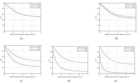
6.4.4 Small Dimension Validation

Fig. 7 shows five plots of ˆpFP for different values of

displacements∆=µn−µn,H0. Indeed, the actual value of∆ is unknown. However, the focus is on the min-imization of ˆpFP. Accordingly, ˆpFP decreases in each

sub-figure of Fig. 7. The actual value of∆ only de-termines how fast ˆpFP decreases. So we can solve the

optimization problem (cf. Eq. 1) by minimizing ˆpFP.

(a) (b)

(c) (d) (e)

Figure 7: Estimation of ˆpFPfor different values of∆andσwith∆=α·v·10−3. The value ofαis 0, 1, 5, 10 and

15 in Fig. 7 a), Fig. 7 b), Fig. 7 c), Fig. 7 d) and Fig. 7 e) respectively.

following values{_0.01,0.05}_{for σ =σ1 =σ2 and} se-lected the following displacements∆=α·_v·₁₀−3_with

α∈ {_{0; 1; 5; 10; 15}}_{andv= [1,}−_1]T_.

7

Optimization

The first strategy is to optimize the feature selec-tion. Optimal features are learned in an unsupervised learning session where an evolutionary optimization framework is applied to search for optimal features. The next strategy is to improve the labeling of test cases through an active learning strategy.

7.1

Evolutionary Optimization

Clustering (and sub-clustering) of test cases is per-formed based on features. Therefore, different cluster-ings for different selections of feature subsets (Φ_m,Φ_s) are possible. Accordingly, a different statistical model is obtained, as it reflects the failure frequencies in clusters. Furthermore, the differential mutual infor-mation (cf. Eq. 31) depends on the statistical depen-dencies and thus changes for different clusterings.

Sec. 6 proposed a calculation formula for the weightswn,0≤n≤N ,of a linear classifier. However,

those formulas still depend on the differential mutual informationI. A desired sensitivity has to be guaran-teed, and thus the hyperplane is adjusted according to the value ofI. It can be shown that for small values of

I, the position of the hyperplane still guarantees a de-sired sensitivity but the false-positive selection prob-ability increases. To minimize the false-positive

selec-tion probability, the differential mutual information has to be maximized, which is the final strategy for solving the constrained optimization problem (cf. Eq. 1).

First, clustering depends on the history-tuples of test cases as, for example, the length of the history-tuples determines the maximum number|_S|K _of clus-ters. Second, feature selection is optimized. All in all, we have summarized that K (number of consid-ered previous regressions) is an optimization param-eter andbs (for coding selected and main features) is

an optimization matrix. However, this is a large-scale high dimensional optimization problem, as there exist many possible settings forKandbs. Thus, [3] and [4]

suggest that the high dimensional optimization prob-lem can be solved in a reasonable time by using evolu-tionary algorithms. Accordingly, an evoluevolu-tionary op-timization framework is applied for solving the men-tioned high dimensional optimization problem. As each setting forK andbs is one possible solution for

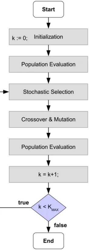
clustering test cases, which is the basis for derivation of a stochastic model, the fitness of this solution can be evaluated by calculating the extracted information I _{in Eq. 31. Thus, the optimal parameter and matrix} setting with the best fitness will survive and will be returned by the evolutionary optimization algorithm. Fig. 8 shows the overall flow chart of the evolu-tionary optimization framework. First of all, a new population consisting of several genotypes is initial-ized. Each genotype stands for a possible setting ofK

andbs . In the next step, the corresponding

phe-notype encodes a stochastic model. Accordingly, the population is evaluated, wherein the fitness of each phenotype is calculated. However, abadfitness is also possible due tobadstatistical properties of the under-lying stochastic model. This means that statistical cal-culations based on the stochastic model that a pheno-type encodes cannot guarantee desired statistical con-fidence bounds. This will be explained in more detail in Sec. 8. Those phenotypes withbadfitness cannot survive and hence are eliminated.

Accordingly, remaining genotypes (phenotypes) are stochastically selected, and successively new genotypes are generated due tocrossoverandmutation

operations. After a certain number of iterations, the phenotype with the best fitness will be selected, and this will be used in the selection algorithm. However, if the population is empty since all phenotypes were ofbadfitness, then the training mode is activated, in which test cases are still executed without running the selection algorithm.

Start

Population Evaluation Initialization

Crossover & Mutation

Population Evaluation

k < K_MAX Stochastic Selection

End k := 0;

true

false k = k+1;

Figure 8: Evolutionary Optimization Framework.

7.2

Active Learning

Our classifier’s conducted decisions can be regarded as hard or even as soft decisions. Once taken, hard

decisions are never changed later on, in contrast to

softdecisions. The test efficiency can be significantly increased by conductingsoft decisions as opposed to

harddecisions.

7.2.1 Hard Decision

[1] performs hard decisions since a selected test case is automatically executed and a once deselected test case is never selected again in the current regression test. In the following passages, the disadvantage of conducting hard decisionswill be explained in detail in relation to classifier decisions.

The linear classifier’s decision depends on the cur-rent estimation of ˆNFN as it calculates the allowed

residual riskpFN ,Limit (cf. Eq 6) of potentially taking

a wrong decision. NˆFN returns the number of

sup-posedly unrevealed system failures that would be de-tected by those already deselected test cases that are elements ofT_Exec. Accordingly, the linear classifier’s decision depends on the decisions it has already taken (T_Exec) and hence it is memory driven.

Each deselected test casetj has an individual

ad-ditional contribution ˆNFN ,j (cf. Eq. 36) to the overall

estimation ˆNFNsuch that the relation in Eq. 35 holds.

ˆ

NFN=

X

∀_tj∈_T

Exec

ˆ

NFN ,j ₍₃₅₎

ˆ

NFN ,j is the product of tj’s failure probabilityx and

the false-negative probabilityP( ˆH =H0|H1) by dese-lectingtjas given in Eq. 36.

ˆ

NFN ,j=P(H1)P( ˆH=H0|H1) (36)

Because of this fact, a deselection of an arbitrary test case can cause that the residual risk pFN ,Limit

reaches zero as ˆNFN increases (cf. Eq. 6). This means

that no more risk (pFN ,Limit = 0) is allowed, and all

remaining test cases have to be consequently selected. Indeed, selecting test cases even if their deselec-tion is allowed according to risk calculadeselec-tions is some-times the better choice. In fact, this is the case if

pFN ,Limit is zero and thus it can be significantly

in-creased by selecting and executing an already dese-lected test case in order to eliminate its risk. When this is done, ˆNFN decreases and hence pFN ,Limit

in-creases and thus a residual risk for further deselec-tions is obtained.

However, the amount∆NˆFNof how much ˆNFNcan

be decreased by selecting an arbitrary test case is sig-nificant. If later more than one test case can be des-elected, and these deselected test cases add the same amount of expected unrevealed system failures∆NˆFN

to ˆNFNis in fact a gain in terms of reducing the

As a result, the regression test efficiency can be in-creased. Therefore, the proposed selection method [1] is extended by asoft decision methodology. So each decision for deselecting a test case is now regarded as asoft decisionthat might be changed later. (We note here that the other way round is impossible since an already selected test case is automatically executed on the system under test and hence deselecting it later does not make sense).

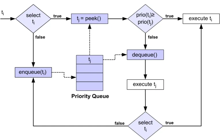
7.2.2 Soft Decision

Fig. 9 shows the logic for managing soft selection de-cisions: Let us assume thatti is the next test case that

is analyzed by the linear classifier. Ifti is deselected,

then it is queued into a priority queue whereby its pri-ority is calculated as given in Eq. 37.

prio(ti) = ˆNFN ,i =P(H1)P( ˆH=H0|H1) (37)

In the other case, ifti is selected then test cases

dese-lected up to this point are analyzed to the end of im-proving the trade-off between the assumed risk and the total number of deselected test cases. As a conse-quence, the most probable failing test case tj is

ob-tained by taking the peek-operation on the priority queue. The priority ofti andtj is compared, and the

test case with the higher priority is selected and exe-cuted on the system under test.

If tj is executed, then it is removed from the set

T_Exec←_T

Exec\tjand added into the setTExec←TExec∪

tj. Furthermore, tj’s state is evaluated eval(tj) and

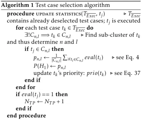
accordingly the empirical failure probabilities of test cases are updated in algorithm 1. Since the calculated failure probabilities are averages of test case evalu-ations, the failure probabilities of those sub-clusters (see Eq. 4) have to be updated where tj is an

ele-ment of them. Accordingly, the failure probabilities of∀_tk∈_T

Execare updated in algorithm 1.

Algorithm 1Test case selection algorithm

procedureupdate statistics(T_Exec,t_j) . T_Exec contains already deselected test cases;tjis executed

foreach test casetk∈TExecdo

∃_!Cn,l=⇒_tk∈_{Cn,l .Find sub-cluster oftk} and thus determinenandl

iftj∈Cn,lthen

pn,l← |_C1_n,l|

P

∀_ti∈_Cn,leval(ti) .see Eq. 4

P(H1)←_pn,l

updatetk’s priority:prio(tk) .see Eq. 37

end if end for

ifeval(tj) == 1then

NT P ←NT P+ 1

end if end procedure

The important point is that even the failure proba-bility ofti is computed again. In most cases,ti would

be deselected. Nevertheless, it could be possible that

the execution oftj has failed, such that a further

sys-tem failure has been found. In such a case, eventi’s

failure probability may have increased such that its deselection has to be checked again by the linear clas-sifier.

All in all, testing efficiency can be significantly in-creased by performing soft selection decisions. The performance of both selection strategies (hard decision

andsoft decision) will be compared in Sec. 9.

8

Learning Phase

The learning phase is of essential importance due to the fact that during this phase, the system reliability is actually learned. Test case selection is a safety-critical binary classification task as probably system failures would remain undetected and hence, a correspond-ing quality measure of wrong decisions is required. Accordingly, risk estimations on probably undetected system failures due to deselection of test cases have to be as accurate as possible. The more the system is learned during a regression test, the more precise the risk estimations are. However, learning a system in terms of understanding its reliability is a costly pro-cess, as it requires test cases to be executed. The fun-damentally important research question is how much training data is enough for safely selecting test cases with a desired sensitivity.

8.1

Statistical Sensitivity Estimation

We have already required a specific sensitivity in the constraint optimization problem (cf. Eq. 1). Accord-ingly, we define the following confidence level in Eq. 38, which is basically driven from the constraint of Eq. 1.

PΨ ≤_γ≥₁−_{α (38)}

Ψ is an estimator for the number of false-negatives ˆ

NFN =Pti∈TEXEC

ˆ

NFN ,i and the bound is given asγ= NT P·pFN ,MAX

1−_{pFN ,MAX} . Ψ =

P

iψi is composed of several

ran-dom variablesψistanding for the distribution of each

ˆ

NFN ,i. ψi’s distribution is complex, since the

individ-ual contribution of a deselected test caseti is given

by ˆNFN ,i =xNpˆFN wherexN isti’s failure probability

and ˆpFNis the corresponding estimated false-negative

probability: The following theorem is already proved in [1] and gives the formula for the false-negative probability estimation.

Theorem 2 (False-Negative Probability). For a given

pththe calculation formula of the false-negative

probabil-ityP( ˆH=H0|H1)has the form

ˆ

pFN =1

2      1 +erf

     

1 √ 2

xN−(xN−pth)e2

I₋

µN

σN

√

e2I₋

1             (39)

wherexN is the failure probability of a test case, whereas

µN, σN are parameters of the probability distribution

enqueue(t_i)

prio(ti)≥

prio(t_j) select

ti

select ti

execute tj

ti

tj

Priority Queue true

false

true

false

execute ti

tj = peek()

true false

dequeue()

Figure 9: The extended concept for conducting soft decisions

These statistics are created on the basis of sam-ple averages, such that the consideration of samsam-ple variances becomes inevitable during the estimation of confidence intervals. For instance, the false-negative probability estimation ˆpFN(see Eq. 39) is composed of

the statisticsxN,µN,σN andI. Therefore, its variance

depends on the individual variances of each statistic, including the sample variance ofxN. Especially the

probability distribution of I is complex as it is non-linearly composed of a set of multivariate distributed Gaussian random variables.

Therefore, we choose the following approach to solving Eq. 38. We simplify the definition of ψi as

follows ψi = ˆpFN ·XN where ˆpFN is assumed to be

a constant value without any distribution. This step simplifies the calculation complexity of Eq. 38 sig-nificantly, as Ψ becomes simply a weighted sum of Gaussian random variables. However, the variance of

ˆ

pFN is of course relevant and should not be easily

ne-glected. Accordingly, we require a maximum confi-dence interval width for ˆpFN such that the estimated

false-negative probability is quite accurate and hence can be assumed to be just like a constant value with-out any statistical deviation. We calculate the confi-dence interval [ ˆp_FN(l); ˆp(_FNu)] and its widthδ= ˆp(_FNu)−_pˆ(l)

FN

and require a maximal confidence interval width of

δmax.

The Wilson score interval [22] delivers confidence bounds for binomial proportions. Therefore, we cal-culate the following confidence intervals [x(nl);xn(u)]

(confidence level: 1−_{α= 99%) for each failure} prob-ability estimationxn,1≤n≤N. Each bound is

conse-quently used for building the bounds of the composed statisticsσ,ΣandI. By doing this, we obtain the fol-lowing bounds: σ(b),Σ(b)andI(b)withb={_{u, l}}_. Ac-cordingly, we calculate ˆp(_FNb) by consequently inserting

the boundsσ(b),Σ(b)andI(b)for the statisticsσ,Σand

Irespectively.

8.2

Criteria for Training

In order to guarantee a statistical bound on the sensi-tivity with a 99% confidence level, the following con-ditions have to be checked.

1. δ≤_δmax

2. PΨ ≤_γ≥₁−_{α= 99%}

If both conditions are fulfilled, then these risk cal-culations in the selection algorithm are reasonably accurate and hence selection decisions can be per-formed. However, if one condition is not fulfilled then the training mode is just active, such that test cases still have to be executed.

9

Industrial Case Study

A German premium car manufacturer constitutes each regression test as being a system release test, and thus the system test takes up to several weeks accord-ing to [5]. However, a first detected system failure makes a system release impossible so optimizing the current regression for achieving high efficiency in re-ducing the regression effort becomes justified.

is no longer possible) and keeping the limited testing time back for fault-revealing test cases decreases the regression test effort significantly. In any case, a final regression test will succeed after further system up-dates have been conducted; this will be constituted as a final release-test that meets the high-quality stan-dards of [5].

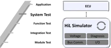
In our industrial case study, we applied our selec-tion method to a producselec-tion-ready controller that im-plements complex networked functionalities for the protection of passengers and other road users. There-fore its test effort is immense, and hence we apply our regression test selection method for accelerating its testing phase. In Fig. 10 the right-hand side of the well-knownV-Model(see [23]) is shown, whereas the focus is on system testing in our case study.

A hardware-in-the-loop simulator (HiL) [24] is used for validating an ECU’s networked complex functionalities as well as its I/O-interaction and its ro-bustness during voltage drops, as it provides an eff ec-tive platform for testing complex real-time embedded systems.

HiL Simulator

ECU

Voltage Bus Comm.

Diagnosis I/O

Module Test Integration Test Function Test System Test Application

Figure 10: A HiL simulator is used for performing the system test.

Further, we selected for the following test case fea-tures for training the machine learning algorithm:

• Name of verified system parts

• Name of a function for which reliability is as-sured

• Number of totally involved electronic control units during the testing of a networked func-tionality

• Error type (broken wire etc.) in hardware ro-bustness tests

• Set of checked diagnostic trouble codes,DTCs • Number of checked diagnostic trouble codes,

DTCs

Since the quality of our selection decisions is hedged on a stochastic level, it can appear that dur-ing different runs of our selection method, a statisti-cal deviation of the false-positive probabilities could occur. Therefore, we constitute several independent runs of a regression test, where we setpFN ,MAX = 1%.

The boxplots and the quantiles of the false-positive probabilities are given in Fig. 11 and in Table 4, re-spectively.

Fig. 11 shows the overall boxplots of the false-positive probabilities achieved during the regression test replications. To compare the hard with the soft decisionstrategy we performed distinct regression test replications where we disabled and enabled the pa-rameter for’soft decision’, respectively.

It can be seen from Fig. 11a) and Fig. 11b) that the average false-positive probability is about 74% and 23% for hardand enabled soft decisionsrespectively. As already mentioned, conductinghard decisionsdoes not allow for global optimization of the trade-off be-tween an already assumed risk and the corresponding number of totally deselected test cases. Global opti-mization hence requires the analysis of all test cases deselected thus far over and over again, and, if neces-sary, the selection of an already deselected test case. Therefore, test cases with a higher failure probabil-ity should be considered again for eventual selection in an ongoing regression test in order to potentially deselect further less risky test cases. As a result, the regression test effort can be reduced much more by applyingsoft decisions.

Furthermore, the condition in Eq. 40 on the false-negative probabilitypFNor on the number of actually

occurring false-negativesNFN was fulfilled in all

con-ducted regression test replications.

pFN ≤pFN ,MAX= 1% or

NFN ≤1

(40)

Our implemented algorithm for selecting test cases runs on a desktop CPU that is specified in Ta-ble 5. We decided to conduct a multithreaded execu-tion of the evoluexecu-tionary algorithm such that the fit-ness of all phenotypes in a population is computed in a multithreaded manner (in total 32 threads). Thus the average CPU load is approximately 95% and the maximum memory allocation is about 4GB. We need a mean analysis time of 0.9s for deciding whether a test case should be selected or not.

10

Conclusion and Future Work