Wage Gap and Employment Status in Indian
Labour Market – Quantile Based
Counterfactual Analysis
Panchanan Das
aReceived: 31.05.2018; Revised: 23.11.2018; Accepted: 25.11.2018
This study examines the extent of wage gap between workers in permanent and tempo-rary jobs but in roughly similar occupation types by evaluating the impact of workers’ characteristics and education. The differential effects of the covariates on wage gap at different locations of the wage distribution are estimated by applying quantile regres-sion model. After estimating the differential effects the relevance of glass ceiling or sticky floor hypothesis has been tested with Indian data. The wage gap between tem-porary and permanent employment is decomposed into endowment effect based on the difference in labour market characteristics and coefficient effect based on the difference in returns for the same characteristics. The study observes that the wage gap between temporary and permanent workers is wider at the upper tail of the distribution not rejecting the glass ceiling hypothesis. The decomposition analysis suggests that the wage gap presents in the Indian labour market primarily because of discrimination measured by the coefficients effects.
JEL codes: C21, D31, I24
Keywords: Employment Structure, Quantile Regression, Earnings Inequality, India
1 Introduction
Increasing earning inequality with a significant increase of temporary employment has been experiencing in almost all countries (both developed and developing) during the past three decades (Levy & Murmane, 1992; Juhn et al., 1993; Gottschalk & Smeeding, 1997;
Banerjee & Piketty,2005;Picchio,2006;Naticchioni et al.,2008;Chancel & Piketty,2017). But, the problem of inequality is more critical in the transitional developing economy, and the analysis of earning distribution with employment structure and other characteristics of the labour market assumes significance both in theoretical and empirical research. This study re-examines the wage gap between permanent and temporary workers engaged in roughly similar type of job by taking productivity enhancing factors like education, training and work experience into account in a transitional developing economy, India, after two and a half decades of economic reforms towards globalisation.
In India, employment has been generated mainly in the form of temporary employment of heterogeneous types during the high growth regime under economic liberalisation. This
study analyses the driving forces behind the dynamics of wage gap with the latest round survey data on employment and unemployment conducted by the National Sample Survey Office (NSSO) in India. We define temporary employment in terms of job status and types of job contract. Casual workers with no written job contract or written job contract for very short period are treated as workers in temporary employment. Temporary workers do not enjoy social security benefits and they are getting wages according to the terms of the daily or periodic work contract. Temporary workers are casual workers and most of them have no written job contract, while permanent workers have written job contract for longer period. Permanent workers enjoy social security benefits and they get wage or salary payment on regular basis.
Workers’ education and skill have normally been treated as the major factors determining the status of employment of a person. The human capital theory suggests that education and training would improve workers’ skills, enabling them to work in the high productive sector for higher wage. It is well documented that better-educated persons are able to earn higher wages, experience less unemployment, and work in more high-status occupations than their less-educated counterparts (Cohn & Addison,1997). But, in a transitional developing economy like India, higher level of education does not provide any guarantee for high status employment. There are some other factors, mostly relating to gender, social, political and other characteristics of a person that may determine the job status and the respective pay structure in the labour market. This study estimates the relative contributions of these factors.
The return to education, the major determining factor of wage earning, may be different in different job status and at different locations of the distribution irrespective of gender and other characteristics of workers. Many empirical studies revealed that the return to education is higher at the top of the wage distribution than the return at the bottom of the distribution (Gonz´alez & Miles,2001;Skyt Nielsen & Rosholm, 2001). There are some studies exploring wage gap between permanent and temporary workers after controlling the effects of education and other characteristics with data from European countries (for example,Picchio (2006); Naticchioni et al.(2008)), but no attempt has been made on the similar issue with Indian data. This study is an attempt to fill this gap in the literature.
We re-examine the nature of wage gap across different locations of wage distribution and look into the role of productivity enhancing characteristics like workers’ education and training in determining the gap. The basic research question is to examine how much the wage gap varies at different locations of the wage distribution by evaluating the impact of workers’ characteristics and education. To find out the differential effects of the covariates on wage at different locations of the wage distribution we have applied the quantile regression model. To examine the wage gap between workers in temporary and permanent employment across wage profile, and to test the relevance of glass ceiling or sticky floor hypothesis1 we have followed Machado and Mata(2005) as suggested in Melly (2005). The wage gap between temporary and permanent employment is decomposed into endowment effect based on the difference in labour market characteristics and coefficient effect based on the difference in returns for the same characteristics.
The study observes that the wage gap between temporary and permanent workers is wider in the upper tail of distribution supporting theglass ceiling hypothesis. The decom-position analysis suggests that the pay gap presents in the Indian labour market primarily because of discrimination measured by the coefficients effects. The rest of the study is organised as follows. Section2describes, in short, the data used in this study. Section3 de-scribes the relevant summary statistics based on the 68thround survey during 2011-12, the latest survey round in India, relating to employment structure and wage earnings. Section
4deals with econometric methodology used in this study. Section5interprets the empirical results on the basis of econometric model described in section4. Section6summarises and concludes.
2 Data
We have used unit level data from 68th rounds survey on employment and unemployment situation in India (Schedule 10) for the period 2011-12 provided by the NSSO. In schedule 10 of the survey round, activity status is classified into 13 groups consisting mainly different forms of self-employment, wage employment and other activities. Self-employed are those who operate their own farm or non-farm enterprises or are engaged independently in a profession or trade. The self-employed are further categorised into own-account workers, employers, and unpaid workers in household enterprises. Wage employment is divided into regular wage employment and casual employment. Regular wage workers are those who work in other’s farm or non-farm enterprises of household or non-household type and get salary or wages on a regular basis, not on the basis of daily or periodic renewal of work contract. This category not only includes persons getting time wage but also persons receiving piece wage or salary and paid apprentices, both full time and part-time. On the other hand, a person working in other’s farm or non-farm enterprises, both household and non-household type, and getting wage according to the terms of the daily or periodic work contract is a casual wage labour. The survey data also provide the nature of job contract as no written job contract, written job contract for 1 year or less, written job contract for more than 1 year to 3 years, and written job contract for more than 3 years. By matching with type of job contract, it is observed that regular wage workers have written job contract for longer period while most of the casual workers have no written job contract at all. Thus, regular wage workers with job contract for longer years are treated as permanent workers and casual wage workers with no written job contract or job contract for very short period as temporary workers.
3 Descriptive Statistics
3.1 Labour market outcomes by level of education
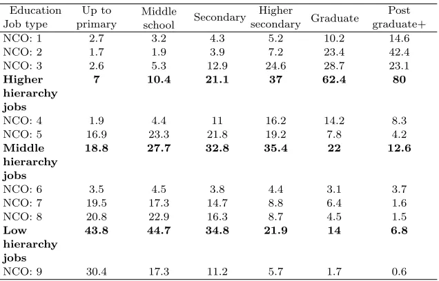
Labour market outcomes in terms of nature of employment and occupation dependent highly on workers’ education and other characteristics. Accumulation of human capital through education, however, is no longer a guarantee of getting better job with higher earning. Many socio-economic and cultural factors restrict the higher educated people to enter into higher hierarchy employment. In this section we have described the labour market outcomes at different levels of education on the basis of available information in the survey data. Wage workers (both permanent and temporary) are engaged in different types of jobs or occupation. In NSSO unit level data, workers’ occupation is classified by national classification of occupation (NCO)2. We have constructed the distributions of wage workers separately for permanent and temporary types3 by occupations as defined in one digit NCO (2004) at different levels of education with the latest available survey round (NSSO 68th round in 2011-12) and are shown in Tables1and 2respectively.
Table 1: Distribution of wage worker in permanent employment with different level of education by occupation type: 2011-12 Education Up to
primary
Middle
school Secondary Higher
secondary Graduate
Post graduate+ Job type
NCO: 1 2.7 3.2 4.3 5.2 10.2 14.6 NCO: 2 1.7 1.9 3.9 7.2 23.4 42.4 NCO: 3 2.6 5.3 12.9 24.6 28.7 23.1
Higher hierarchy jobs
7 10.4 21.1 37 62.4 80
NCO: 4 1.9 4.4 11 16.2 14.2 8.3 NCO: 5 16.9 23.3 21.8 19.2 7.8 4.2
Middle hierarchy jobs
18.8 27.7 32.8 35.4 22 12.6
NCO: 6 3.5 4.5 3.8 4.4 3.1 3.7
NCO: 7 19.5 17.3 14.7 8.8 6.4 1.6 NCO: 8 20.8 22.9 16.3 8.7 4.5 1.5
Low hierarchy jobs
43.8 44.7 34.8 21.9 14 6.8
NCO: 9 30.4 17.3 11.2 5.7 1.7 0.6 Note: Higher hierarchy jobsinclude NCO 1 (Legislatures and executives), NCO 2 (Professionals), and NCO 3 (Technicians & associate professionals);Middle hierarchy jobsinclude NCO 4 (Clerks) and NCO 5 (Service workers and shop and market sales workers);Low hierarchy jobsinclude NCO 6 (Skilled agricultural and fishery workers), NCO 7 (Craft and related trades workers), and NCO 8 (Plant and machinery operators and assemblers); and NCO 9 includes elementary occupations.
Source: Author’s calculation with 68thround unit level NSSO data
2 In one digit classification, NCO (2004) describes the following occupations. NCO 1: Legislatures, ex-ecutives, NCO 2: Professionals, NCO 3: Technicians & associate professionals, NCO 4: Clerks, NCO 5: Service workers and shop and market sales workers, NCO 6: Skilled agricultural and fishery workers, NCO 7: Craft and related trades workers, NCO 8: Plant and machinery operators and assemblers, and NCO 9: Elementary occupations
Distribution of workers in permanent employment by types of occupations at a particular level of education is not similar to that of the temporary workers. The proportion of higher hierarchy jobs (legislatures, executives, professionals and associate professionals) increases with the increase in education both in permanent and temporary employment, but in the case of temporary employment the relationship is not so strong. The incidence of higher hi-erarchy jobs is higher in permanent employment than in temporary employment with same level of education. For example, about 80 per cent of post-graduate workers in permanent employment are engaged in high hierarchy jobs, while the respective share in temporary employment is just above 20 per cent. Middle hierarchy jobs (clerks and service workers in sales) in permanent employment are concentrated among workers with secondary and higher secondary levels of education. But, the similar kind of jobs in temporary employment are centred at education level higher secondary and graduate. The incidence of low hierarchy jobs (skilled agricultural workers, crafts and related trades workers, and machinery opera-tors) is high among permanent workers at education up to secondary level, but it is notably high at any education level among temporary workers. Around 41 per cent of the graduate and 29 per cent of the post-graduate workers in temporary employment are in low hierarchy jobs.
Table 2: Distribution of wage worker in temporary employment with different level of education by occupation type: 2011-12 Education Up to
primary
Middle
school Secondary Higher
secondary Graduate
Post graduate+ Job type
NCO:1 1.4 2.4 3 2.7 3.6 16.7
NCO:2 0.5 0.6 1 2 3.3 4.2
NCO:3 0.5 1.2 1.4 2.8 7.9 0
Higher hierarchy jobs
2.4 4.1 5.4 7.6 14.8 20.8
NCO:4 0.3 0.6 1.1 1.1 4.2 4.2
NCO:5 3.3 5.4 7.2 9.2 8.2 0
Middle hierarchy jobs
3.6 5.9 8.4 10.3 12.4 4.2
NCO:6 3.3 5.6 6.2 7.9 6.7 8.3
NCO:7 23.7 28 29.1 23.2 29.1 16.7
NCO:8 4.5 6.6 6.9 6.9 5.8 4.2
Low hierarchy jobs
31.5 40.3 42.2 37.9 41.5 29.2
NCO:9 62.5 49.7 44 44.2 31.2 45.8
Note: Higher hierarchy jobsinclude NCO 1 (Legislatures and executives), NCO 2 (Professionals), and NCO 3 (Technicians & associate professionals);Middle hierarchy jobsinclude NCO 4 (Clerks) and NCO 5 (Service workers and shop and market sales workers);Low hierarchy jobsinclude NCO 6 (Skilled agricultural and fishery workers), NCO 7 (Craft and related trades workers), and NCO 8 (Plant and machinery operators and assemblers); and NCO 9 includes elementary occupations.
Source: Author’s calculation with 68thround unit level NSSO data
techni-cians, professionals, or clerks. All permanent workers with highest education are not in high profile occupations like executives, professionals or associate professionals. A noticeable part of them are in clerical jobs, or in sales services, or even in agricultural activities. The incidence of better quality jobs increases with the increase in education level in permanent employment, but the changing pattern of jobs with education is not systematic. Temporary workers, on the other hand, are concentrated mainly in low profile jobs and majority of them are in elementary occupation irrespective of their level of education (Table2). Major part (62.5 per cent) of the wage workers with education up to primary level who are in tem-porary employment are absorbed in elementary occupation. Surprisingly enough, nearly 46 per cent of the post-graduates and 31 per cent of the graduates in temporary jobs are forced to accept elementary occupation in the Indian labour market.
3.2 Observed wage gap between permanent and temporary employment
The difference in labour market outcomes in the form of occupational and employment status between permanent and temporary workers has serious implications in explaining wage distribution of these two types of workers. Before analysing wage distribution in terms of workers’ education and employment characteristics we have looked at the observed wage at different locations of the wage distribution. Daily wages for permanent and temporary workers at percentiles 10, 25, 50, 75 and 90 of the wage distribution have been estimated on the basis of sample observations taken from 68thround survey by using appropriate sample weights obtained from the multiplier provided in the data to make estimates population representative. The estimated values are shown in Table3.
Table 3: Wages in temporary and permanent employment at
different locations of wage distribution: 2011-12
Location of wage distribution
Daily wage (Rs.)
Permanent worker Temporary worker
Q10 100 80
Q25 150 100
Q50 300 150
Q75 643 200
Q90 967 250
Q90 / Q10 9.7 3.1
Mean 397 141
Standard error 4.03 0.67
Source:Author’s calculation with 68thround unit level NSSO data
inequality among temporary workers. The estimated standard errors of daily wages of these two groups also suggest the similar phenomenon.
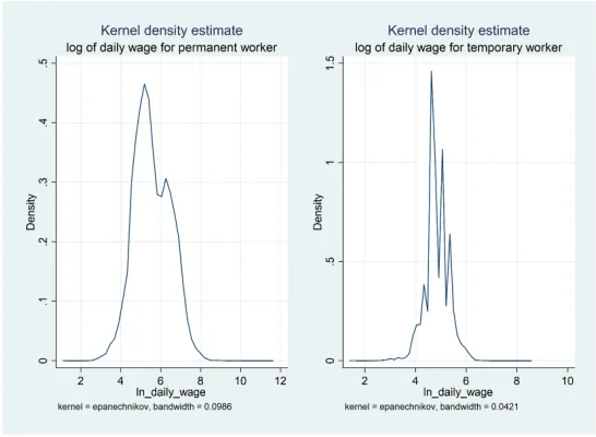
The Kernel density estimates across the employment groups provide a better idea about the existing wage gap between workers in permanent and temporary employment. The density functions of daily wages for workers in temporary and permanent employment have been estimated by using an Epanechinov kernel estimator. As is shown by the shape of the estimated Kernel density function of log values of daily wages (Figure1), the distribution of wage in permanent employment is significantly different from the wage distribution in temporary employment. The estimates reveal a larger proportion of the permanent workers to be in the higher wage levels. The two-sample Kolmogorov-Smirnov test is used to compare the observed cumulative distribution function for log values of daily wages with the normal distribution. The Kolmogorov-Smirnov Z-statistic is computed from the largest difference between the empirical and theoretical cumulative distribution functions. The test rejects the null hypothesis that the wages of the permanent and the temporary workers follow the same distribution at less than 1 per cent level of significance (p−value= 0.001).
Figure 1: Kernel density function of log of daily wage
Table 4: Average wage and Gini index of daily wage of permanent and temporary workers across education level: 2011-12
Education level Permanent worker Temporary worker Average daily
wage (Rs.)
Gini index Average daily wage (Rs.)
Gini index
Not literate 163 0.38 128 0.23
Below primary 204 0.36 125 0.22
Primary level 192 0.37 146 0.25
Middle school level 221 0.38 156 0.28
Secondary level 305 0.4 159 0.26
Higher secondary 369 0.41 151 0.26
Diploma 486 0.37 222 0.31
Graduate 634 0.42 176 0.27
Post-graduate and above 840 0.4 151 0.21
All 397 0.49 141 0.25
Source:Author’s calculation with 68thround unit level NSSO data
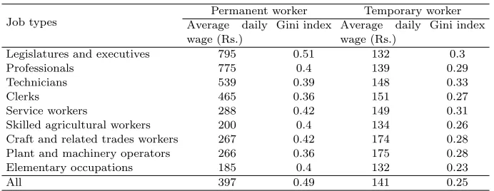
The extent of wage inequality is not the same in permanent and temporary employment, and it varies across workers’ education level and job types. Wage distribution in permanent employment is more unequal than in temporary employment, and the incidence of inequality is different at different level of workers’ education as well as in different types of jobs. The relationship between wage inequality and workers’ education is different in permanent employment from that in temporary employment. In permanent employment, the incidence of wage inequality is the highest among graduate workers and the lowest among workers with education below primary level. In temporary employment, on the other hand, the extent of wage inequality is the highest among diploma holders and the lowest among post-graduate workers. However, there is no specific pattern of relationship between wage inequality and job hierarchy is observed both in permanent and temporary employment. Gini index of daily wages is the maximum in the top ranking jobs followed by services workers and trade workers in permanent employment. In temporary employment, on the other hand, Gini index is the highest among technicians and the lowest in elementary occupations.
Table 5: Average wage and Gini index of daily wage of permanent and temporary workers across education level: 2011-12
Job types
Permanent worker Temporary worker Average daily
wage (Rs.)
Gini index Average daily wage (Rs.)
Gini index
Legislatures and executives 795 0.51 132 0.3
Professionals 775 0.4 139 0.29
Technicians 539 0.39 148 0.33
Clerks 465 0.36 151 0.27
Service workers 288 0.42 149 0.31
Skilled agricultural workers 200 0.4 134 0.26 Craft and related trades workers 267 0.42 174 0.28 Plant and machinery operators 266 0.36 175 0.28 Elementary occupations 185 0.4 132 0.23
All 397 0.49 141 0.25
4 Econometric model
This paper analyses wage gap (as shown in Tables3 to5) between permanent and tem-porary employment in the Indian labour market in two steps. In the first step, the wage equation is estimated at the selected quantiles of the wage distribution. In the second step, wage gaps at the selected quantiles are estimated and decomposed into endowment effects originated from the difference in the productive characteristics of the workers, and differen-tial returns effects initiated from the differences in returns to the productive characteristics following quantile decomposition method. This method enables us to explore the potential effects on the shape of the distribution in addition to the shift of the distribution due to the shift of the covariates. The quantile regression model has been popularised after the publication of Koenker and Bassett (1978, 1982). The literature has been developed fur-ther byMachado and Mata (2005);Melly(2005); Firpo et al.(2009); Fortin et al.(2011);
Lechmann and Schnabel (2012); Magnani and Zhu (2012); Chi and Li (2014) along with other scholars to apply quantile regression in decomposition analysis of wage distribution. Quantile regression has been used in many empirical research relating to labour market discrimination because it has some advantages over the ordinary least square4. Quantile regression is more robust to non-normal errors and outliers. It allows to consider the impact of a covariate on the entire distribution of the dependent variable, daily wage in our model, not merely its conditional mean.
In quantile regression framework we estimate the following wage regression equation:
lnwi = Xiβ(θ) +´ i (1)
Here, wi is daily wage of workeri, Xi is the vector of covariates including job types, education, experience, and gender of workeri,βis the coefficient vector,θrepresents quantile of the wage distribution andi is the idiosyncratic error.
The population conditional quantile distribution of (1), for allθgiven the set of covariates X is
Qθ(lnwi|Xi) = X´iβ(θ) (2) Here, the underlying assumption is Qθ(i|Xi) = 0 ∀ θ ∈ (0,1). Thus, equation (1) becomes
lnwi = Qθ(lnwi|Xi) + i (3) Equation (3) states that the unconditional quantile wage is equal to its wage conditional on the vector of explanatory variables at the same quantile plus the random error. The coefficient vectorβ(θ) at quantileθcan be estimated by minimising the following objective function (Koenker & Bassett, 1978):
ˆ
β(θ) = argmin β
"
1 n
n
X
i=1
ρθ(lnwi − Xiβ)
!#
(4)
Here, ˆβ(θ) is calledθthregression quantile, for any quantileθ∈(0,1).
The objective function denotes the loss associated with the prediction errors. Quantile regression minimizes a sum that gives asymmetric penalties (1−θ)|| for over prediction andθ||for under prediction:
ρθ() =
(
θ , if >0. (θ−1), if <0.
Thus, the θth quantile regression estimators, ˆβ(θ) are chosen by solving the following problem
ˆ
βt(θ) = argmin β
X
i∈{i:lnwi≥Xiβ}
θ|lnwi−Xiβ| + X i∈{i:lnwi<Xiβ}
(1−θ)|lnwi−Xiβ|
(5)
This non-differentiable function could be minimised by applying the simplex method. The median regression, least-absolute-deviations regression, is obtained by minimising
ˆ
β(0.5) = X i
|lnwi − Xiβ| (6)
The median-regression line, must pass through the pair of data points with half of the remaining data lying above the regression line and the other half falling below. We have used bootstrap standard errors in estimating the conditional distribution of wages for given Xi andθ by applying the principle described in (4) or, (5):
d
lnwi = X´iβ(θ)ˆ (7)
The estimated coefficient vector measures the rates of return to the corresponding co-variates at the selected quantile of the conditional wage distribution. Under some regularity conditions, the estimated conditional quantile function is a consistent estimator of the pop-ulation conditional quantile function, uniformly inθ (Koenker & Bassett, 1978; Hendricks & Koenker,1992).
After estimating the model given in (1) we decompose the wage differences at selected quantiles of the wage distribution between workers in permanent and temporary jobs into the component due to labour market characteristics and the component due to the differences in returns by followingMelly(2005). This method is an extension to the counterfactual wage decomposition approach of Oaxaca (1973) to quantile regression and provides a general strategy for simulating marginal distributions from the quantile regression process. The Oaxaca decomposition fails to provide information about the whole distribution (Magnani & Zhu, 2012; Chi & Li, 2014; Ahmed & McGillivray, 2015). Machado and Mata (2005) proposed a quantile-based decomposition method, which combines quantile regression with bootstrap approach. Melly (2005) modified the methodology developed in Machado and Mata(2005) by decomposing the wage differences at different quantiles of the unconditional distribution.
the distributions of workers’ characteristicsX and wage W conditional onX respectively in k ∈ (0,1) and j ∈ (0,1). We estimate the conditional distribution by using quantile regression model.
The unconditional wage distributions of workers in permanent and temporary employ-ment are obtained from the estimated conditional distribution in the following way:
FWh0|0i(W) =
Z
FW0(W|X)dFX0(X) (8)
FWh1|1i(W) =
Z
FW1(W|X)dFX1(X) (9)
Let we define
FWhj|ki(W) =
Z
FWj(W|X)dFXk(X) (10) as the counterfactual distribution of wages of workers’ groupj if they have the character-istics of workers’ group k5. Therefore, the counterfactual wage distribution of workers in permanent employment is
FWh0|1i(W) =
Z
FW0(W|X)dFX1(X) (11)
This distribution is constructed by integrating the conditional distribution of wages for workers in permanent employment with respect to the distribution of characteristics of those in temporary employment. The counterfactual distribution is estimated by using the unconditional distribution, and by replacing the estimated parameters of the distribution or the characteristics of permanent workers with those of temporary workers.
We define the distributional effect on wages between these two groups of workers as D(W) = FWh0|1i(W) − FWh0|0i(W) (12)
The quantile measure of the distributional effect6 shown in (12) is
Q(θ) = QWh0|1i(Q) − QWh0|0i(Q) (13)
If workers in temporary employment are in treatment group (1) and workers in permanent employment are in control group (0), the quantile treatment effect on the treated is obtained from the counterfactual distributions as
QT ET = QWh1|1i(Q) − QWh0|1i(Q) (14)
5As this distribution is not derived from any observable population, it is called counterfactual distribution. 6The quantile wage function, the inverse of the wage distribution function,F−1
W (θ), evaluated atθ, 0< θ <1
is defined as
QWhj|ki(θ) = inf{W:FWhj|ki(W)≥θ}, 0< θ <1
Therefore, the quantile decomposition,
QWh0|0i(Q) − QWh1|1i(Q) = QWh0|0i(W) − QWh0|1i(W) +
QWh0|1i(W) − QWh1|1i(W)
(15)
Or,
Q(Xi,0, β0, θ) − Q(Xi,1, β1, θ) =
Qθ(X0,β0,θ)−Qθ(X1,β0,θ)
+
Qθ(X1,β0,θ)−Qθ(X1,β1,θ)
(16)
The first component of wage penalty measures the wage gap because of the differences in workers’ characteristics and the second component measures the difference in the returns given their job characteristics between workers in temporary and permanent employment. 5 Empirical results
5.1 Estimation of quantile regression
It is clear from the descriptive statistics as shown in section3that the wage gap between permanent and temporary employment depends partly on the differences in labour market characteristics like workers’ education and occupation. This section analyses the estimated wage penalty of the temporary workers at different locations of the wage distribution. To find out how workers’ education and other characteristics contribute to wage penalty to temporary workers, the wage regression is estimated at quantiles 0.10, 0.25, 0.50, 0.75, and 0.90 denoted respectively byQ10,Q25,Q50,Q75, andQ90. We have taken log values of daily
wages as dependent variable and variables relating to human capital, employment, industry, and region along with gender and person specific other factors like ethnic characters as covariates.
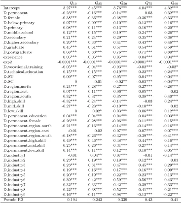
The estimated results based on quantile regression model of the wage distribution are shown in Table6. The intercept term shows the conditional log wage for workers at different quantiles of the wage distribution in the sample irrespective of their level of education, job contracts, payment types and other characteristics of the workers. A huge difference in wage between upper quantile and lower quantile is observed. While workers in temporary employment enjoy wage premium up to median level, a significant wage penalty for them is observed at the top of the distribution. The estimated coefficients of the dummy variable for permanent workers (D permanent) at different quantiles reject the hypothesis ofsticky floors. As revealed by the negative coefficients of gender dummy (D female), women workers have earned lower wage than the men workers and the gender gap is more at the lower tail of the distribution.
The level of education has favourable effect on wage income as expected. To estimate how workers’ education has had impact on wage earnings we have taken workers without any formal education as a reference group and compare wage earnings across workers with different levels of education by incorporating education dummies. As shown in Table 6, return to education increases with education level supporting the hypotheses put forward in the human capital theory, and the return to education at post graduate level is the highest at 25th quantile of the wage distribution. The return to education at the upper tail is significantly higher than that at the lower tail of the wage distribution irrespective of the level of education. However, the effect of experience on wage is roughly similar across different location of the distribution. Wage premium for technical education is the highest at 90th quantile. The wage gap among workers because of the differences in technical know-how may be because of skill biased technological change during the post-liberalisation period.
Table 6: Quantile estimates of conditional earnings
Q10 Q25 Q50 Q75 Q90 Intercept 3.27*** 3.45*** 3.76*** 4.04*** 4.32*** D permanent -0.23*** -0.16*** -0.14*** 0.03 0.32*** D female -0.38*** -0.36*** -0.38*** -0.36*** -0.33*** D below primary 0.07*** 0.09*** 0.10*** 0.13*** 0.16*** D primary 0.08*** 0.11*** 0.13*** 0.16*** 0.20*** D middle school 0.12*** 0.15*** 0.19*** 0.24*** 0.26*** D secondary 0.21*** 0.24*** 0.29*** 0.35*** 0.38*** D higher secondary 0.26*** 0.33*** 0.41*** 0.43*** 0.46*** D graduate 0.45*** 0.61*** 0.57*** 0.54*** 0.59*** D postgraduate 0.68*** 0.83*** 0.76*** 0.71*** 0.80*** experience 0.05*** 0.05*** 0.05*** 0.04*** 0.04*** exp2 -0.0001*** -0.0001*** -0.0001*** -0.0001*** -0.0001*** D vocational training -0.05*** -0.04*** -0.03*** -0.02*** -0.02* D technical education 0.15*** 0.15*** 0.19*** 0.22*** 0.24*** D ST 0.09*** 0.07*** 0.05*** 0.04*** 0.04*** D SC 0 -0.01 -0.02** -0.03*** -0.04*** D region north 0.24*** 0.28*** 0.27*** 0.27*** 0.28*** D region east 0.07*** 0.11*** 0.06*** 0.05*** 0.02 D region south 0.32*** 0.37*** 0.35*** 0.38*** 0.40*** D high skill -0.32*** -0.24*** -0.14*** -0.03 0.24*** D mid skill -0.27*** -0.23*** -0.19*** -0.10*** 0.02 D low skill 0 0.02* 0.03*** 0.06*** 0.12*** D permanent education 0.04*** 0.04*** 0.04*** 0.04*** 0.03*** D permanent female -0.26*** -0.28*** -0.06*** 0.11*** 0.15*** D permanent region north -0.21*** -0.16*** -0.14*** -0.14*** -0.16*** D permanent region east -0.01 0.02 0.07*** 0.07*** 0.07*** D permanent region south -0.18*** -0.26*** -0.32*** -0.39*** -0.41*** D permanent high skill 0.49*** 0.46*** 0.48*** 0.44*** 0.16*** D permanent mid skill 0.25*** 0.26*** 0.31*** 0.27*** 0.14*** D permanent low skill 0.14*** 0.11*** 0.12*** 0.10*** 0.05*** D industry1 -0.01 0.04** 0.07*** -0.01 -0.14*** D industry2 0.23*** 0.19*** 0.19*** 0.12*** 0.03 D industry3 0.23*** 0.31*** 0.47*** 0.45*** 0.29*** D industry4 0.19*** 0.16*** 0.17*** 0.16*** 0.09*** D industry5 0.20*** 0.19*** 0.22*** 0.23*** 0.13*** D industry6 0.39*** 0.42*** 0.59*** 0.56*** 0.43*** D industry7 0.32*** 0.33*** 0.42*** 0.39*** 0.33*** D industry8 0.22*** 0.38*** 0.52*** 0.41*** 0.21*** D industry9 -0.16*** -0.11*** -0.08*** -0.13*** -0.22***
Pseudo R2 0.194 0.243 0.339 0.43 0.41
Note: *** significant at less than 1 per cent level, ** significant at 5 per cent level, the rest are statistically insignif-icant. Industry dummies are constructed on the basis of one digit NIC 2008. Accordingly Industry0: Agriculture, mining and quarrying; Industry1: Manufacturing; Industry2: Electricity, gas; Industry3: Steam and air conditioning supply; Industry4: Water supply; sewerage, waste management and remediation activities; Industry5: Construction; Industry6: Wholesale and retail trade; repair of motor vehicles and motorcycles; transportation and storage; Indus-try7: Accommodation and food service activities; Industry8: Information and communication; financial and insurance activities; Industry9: Real estate activities; professional, scientific and technical activities; administrative and support service activities; public administration and defence; compulsory social security; education; human health and social work activities
Source: Author’s estimation with unit level data from 68throunds of NSSO.
jobs earn less wages compared to wage earnings of similar type of workers in elementary employment, and the temporary-permanent wage gap is more prominent at median of the distribution. Industry specific fixed effects have also been incorporated in determining wage gap between temporary and permanent workers are estimated by using industry dummies taking agro-based industries as the reference industry group. Estimated coefficients of the dummies measure the unobserved heterogeneity across industry groups that have significant effect on wages.
5.2 Decomposition of wage gap
By followingMelly(2005), wage gap between workers in permanent and temporary em-ployment is decomposed into endowment and coefficient effects at selected locations of wage distribution in a quantile regression framework. The sample data used contain 66,204 wage workers among which 39,789 are in permanent employment and 26,415 are in temporary employment. To look into gender differences in wage gap we also decompose the raw dif-ference separately for men and women workers. The estimated results shown in Table 7
highlight that workers in temporary employment roughly similar to those in permanent employment fall behind the latter more at the top of wage distribution.Wage gap presents and it increases monotonically towards the right tail of the distribution not rejecting the
glass ceiling hypothesis. Wage penalty for temporary workers persists in Indian labour mar-ket primarily because of coefficients effect. However, at the lower end of the distribution, the major part of the wage difference could be explained by the differences in productive endowments between permanent and temporary workers. Raw wage difference between per-manent and temporary workers among women is negative at 10th quantile implying that women temporary workers earning very low wage enjoy wage premium.
Table 7: Machado-Mata decomposition of wage gap
All workers Q10 Q25 Q50 Q75 Q90
Raw difference 0.131 0.432 0.811 1.135 1.321 Characteristics 0.129 0.089 0.123 0.147 0.236 Coefficients 0.003 0.344 0.688 0.988 1.085
Women workers
Raw difference -0.159 0.136 0.687 1.319 1.618 Characteristics 0.141 0.118 0.162 0.291 0.573 Coefficients -0.3 0.017 0.525 1.029 1.045
Men workers
Raw difference 0.146 0.463 0.803 1.114 1.29 Characteristics 0.045 0.064 0.083 0.124 0.2 Coefficients 0.101 0.399 0.72 0.99 1.09 Source: Author’s estimation with unit level data from 68th rounds of NSSO.
6 Summary and conclusions
at any education level among temporary workers.
Wage distribution in permanent employment is more unequal than in temporary em-ployment, and the incidence of inequality is different at different level of workers’ education as well as in different types of jobs. Wage gap presents at every location of the wage distri-bution and the extent of the gap becomes wider as we move from bottom end to top end of the distribution. Wage gap increases with the level of workers’ education and it is extremely high in higher hierarchy jobs.
While workers in temporary employment enjoy wage premium up to median level, a significant wage penalty for them is observed at the top of the distribution rejecting the hypothesis ofsticky floors. Return to education increases with education level supporting the hypotheses put forward in the human capital theory. The return to education at the upper tail is significantly higher than that at the lower tail of the wage distribution irrespective of the level of education. The wage gap, as observed in this study, among workers because of the differences in technical know-how may be because of skill biased technological change during the post-liberalisation period.
Workers in Scheduled Tribes earn more daily wage as compared to workers from upper caste at every location of the wage distribution and the gap is higher at the lower end. Persons in temporary employment working in Southern region states enjoy wage premium at the greatest extent compared to those working in Western part of the country. However, the pay gap between Western and Eastern states is very low.
References
Ahmed, S., & McGillivray, M. (2015). Human Capital, Discrimination, and the Gender Wage Gap in Bangladesh. World Development, 67, 506–524. doi:10.1016/j.worlddev.2014.10.017
Banerjee, A., & Piketty, T. (2005). Top Indian Incomes, 1922–2000. World Bank Economic Review,19(1), 1-20. doi:10.1093/wber/lhi001
Chancel, L., & Piketty, T. (2017). Indian income inequality, 1922-2014 From British Raj to Billionaire Raj? (Working Paper Series No. 11). World Inequality Database.
http://wid.world/document/chancelpiketty2017widworld/.
Chi, W., & Li, B. (2014). Trends in China’s Gender Employment and Pay Gap: Estimating Gender Pay Gaps with Employment Selection. Journal of Comparative Economics,
42(3), 708– 725. doi:10.1016/j.jce.2013.06.008
Cohn, E., & Addison, J. T. (1997). The Economic Returns to Lifelong Learning (Working Paper No. B-97-04). Division of Research, University of South Carolina College of Business Administration.
Firpo, S., Fortin, N., & Lemieux, T. (2009). Unconditional Quantile Regressions. Econo-metrica,77(3), 953–973. doi:10.3982/ECTA6822
Fortin, N., Lemieux, T., & Firpo, S. (2011). Decomposition Methods in Economics. In O. Ashenfelter & D. Card (Eds.),Handbook of labor economics, (4a) (p. 1–102). El-sevier, Amsterdam.
Gonz´alez, X., & Miles, D. (2001). Wage Inequality in a Developing Country: Decrease in Minimum Wage or Increase in Education Returns. Empirical Economics, 1(26), 135–148. doi:10.1007/s001810000056
Gottschalk, P., & Smeeding, T. (1997). Cross-national Comparisons of Earnings and Income Inequality. Journal of Economic Literature,2(35), 633–687.
Hendricks, W., & Koenker, R. (1992). Hierarchical Spline Models for Conditional Quantiles and the Demand for Electricity. Journal of the American Statistical Association,
417(87), 58–68. doi:10.2307/2290452
Juhn, C., Murphy, K., & Pierce, B. (1993). Wage Inequality and the Rise in Returns to Skill. Journal of Political Economy,3(101), 410–441. doi:10.1086/261881
Koenker, R., & Bassett, G. (1978). Regression Quantiles. Econometrica, 1(46), 33-50. doi:10.2307/1913643
Koenker, R., & Bassett, G. (1982). Robust Tests for Heteroscedasticity Based on Regression Quantiles. Econometrica,1(50), 43-61. doi:10.2307/1912528
Lechmann, D. S., & Schnabel, C. (2012). Why is There a Gender Earnings Gap in Self-employment? A Decomposition Analysis with German Data.IZA Journal of European Labor Studies,6(1), 1-25. doi:10.1186/2193-9012-1-6
Levy, F., & Murmane, R. J. (1992). U.S. Earnings Levels and Earnings Inequality: A Review of Recent Trends and Proposed Explanations. Journal of Economic Literature,3(30), 1333–1381.
Magnani, E., & Zhu, R. (2012). Gender Wage Differentials among Rural–urban Migrants in China. Regional Science and Urban Economics, 5(42), 779–793. doi:10.1016/j.regsciurbeco.2011.08.001
Melly, B. (2005). Decomposition of Differences in Distribution using Quantile Regression.
Labour Economics,4(12), 577-590. doi:10.1016/j.labeco.2005.05.006
Mueller, R. (2000). Public- and Private-Sector Wage Differentials in Canada Revisited.
Industrial Relations,3(39), 375–400. doi:10.1111/0019-8676.00173
Naticchioni, P., Ricci, A., & Rustichelli, E. (2008). Wage Inequality, Employment Struc-ture and Skill-biased Change in Italy. Labour, s1(22), 27-51. doi: 10.1111/j.1467-9914.2008.00416.x
Oaxaca, R. (1973). Male–female Wage Differential in Urban Labour Market. International Economic Review,3(14), 693–709. doi:10.2307/2525981
Picchio, M. (2006). Wage Differentials and Temporary Jobs in Italy (UCL Discussion Paper No. 33). Departement des Sciences Economiques. https://pure.uvt.nl/ws/ portalfiles/portal/1439134/2006-33.pdf.
Poterba, J. M., & Rueben, K. S. (1994). The Distribution of Public Sector Wage Premia: New Evidence Using Quantile Regression Methods(Working Paper No. 4734). NBER. doi:10.3386/w4734