Information Technology and Control 2017/1/46 100
A Two-Phase Optimization Method
for Solving the Multi-Type Maximal
Covering Location Problem in
Emergency Service Networks
ITC 1/46
Journal of Information Technology and Control
Vol. 46 / No. 1 / 2017 pp. 100-117
DOI 10.5755/j01.itc.46.1.13853 © Kaunas University of Technology
A Two-Phase Optimization Method for Solving the Multi-Type Maximal Covering Location Problem
in Emergency Service Networks
Received 2016/12/22 Accepted after revision 2017/02/14
http://dx.doi.org/10.5755/j01.itc.46.1.13853
Zorica Stanimirović, Stefan Mišković
Faculty of Mathematics, University of Belgrade, Studentski trg 16/IV, 11 000 Belgrade, Serbia e-mails: [email protected]; [email protected]
Darko Trifunović, Veselin Veljović
Faculty of Security Studies, University of Belgrade, Gospodara Vučića 50, 11 000 Belgrade, Serbia e-mails: [email protected]; [email protected]
Corresponding author: [email protected]
are adapted to the characteristics of the considered problem. The RVNS-LP approach is evaluated on real-life instances obtained from two networks of police units in Montenegro and Serbia, and randomly generated test instances of larger dimensions. Experimental evaluation shows that the proposed RVNS-LP reached all opti-mal solutions on all real-life test instances in very short CPU time. On generated test instances, the RVNS-LP also returned optimal solutions in all cases, within short running times and significant time savings compared to CPLEX solver. The mathematical model and the proposed two-phase optimization method may be applica-ble in the design and management of various emergency-service networks.
KEYWORDS: variable neighborhood search, linear programming, emergency service network, maximal covering location problem.
Introduction
Covering models are one the most popular facility lo-cation models in the literature, due to their numerous applications in practice, especially for locating ser-vices and emergency facilities. Many of real-life prob-lems, such as determining the number and locations of public schools, police stations, fire stations, mili-tary bases, medical centers, post offices, bank branch-es, shopping centers, satellite or radar installations, etc., can be formulated as covering problems [11]. In general, covering problems assume a set of cus-tomers and a set of potential locations for estab-lishing facilities. In most of covering problems, it is required that each customer should be served by at least one facility within a given critical distance, de-noted as covering radius. However, in many practical applications, located resources are not sufficient to cover all customers with the desired level of cover-age. This was a motivation for Church and ReVelle [5] to propose a Maximal Covering Location Problem (MCLP). The MCLP model maximizes the amount of demand covered within the acceptable service distance by locating a fixed number of facilities. The MCLP has showed to be one of the most exploited facility location models from both theoretical and practical points of view. Starting from the work of Church and ReVelle [5], many variants of the MCLP are presented in the literature up to now. White and Case [29] considered the case of MCLP in which de-mands of all customers are equal, with the goal to find the maximal number of covered customer (demand) nodes. A steepest descent heuristic was proposed in [29] as a solution method to this variant of MCLP. Klastorin [14] showed that MCLP can be formulated as Generalized Assignment Problem (GAP). The vari-ant of MCLP on the plane was considered by Church
[6], Drezner [9], and Watson-Gandy [28]. Daskin [8] introduced the maximal coverage location model as one of the variants of set covering model. Probabi-listic variant of the MCLP was proposed by ReVelle and Hogan [23], where each potential facility location has assigned a value measuring the probability that a facility will be established on that location. ReVelle et al. [21] proposed a Maximal Conditional Covering Problem, where customer locations need to be cov-ered by facilities at a given coverage radius, while fa-cility locations themselves are supposed to be covered with a different coverage radius by other facilities, in order to provide secondary support. A generalization of MCLP was introduced by Berman and Krass [3], who involved multiple set of coverage levels with the degree of coverage being a non-increasing step func-tion of the distance to the nearest established facility. A general class of covering problems was proposed by Hocbaum and Pathria [13] as the class of problems of maximum k-coverage, and MCLP may be observed as its special case. Another generalization of MCLP is the Multimode Covering Location Problem intro-duced in [7], which deals with locating a given num-ber of different types of facilities, with a limitation of the number of facilities sharing the same location. A review of papers related to the MCLP and its variants can be found in [10, 15, 24].
in-Information Technology and Control 2017/1/46 102
cidents, and each city has assigned information on the expected number of incidents of each type, obtained from the statistical data. Different types of cy units are available, and for each type of emergen-cy unit, it is defined for which types of incident this type of unit is trained to react. A hierarchy among emergency unit types is introduced, meaning that an emergency unit of a certain type can react to inci-dent types handled by emergency units of lower lev-el, but also to some additional types of incidents. The number of available emergency units of each type are limited. The goal of the considered problem is to choose locations for establishing emergency units of each type, such that the number of all covered inci-dents is maximized. We will refer to the problem as the Multi-Type Maximal Covering Location Prob-lem (MTMCLP). To the best of our knowledge, there are no previously published work on this type of gen-eralization of the MCLP.
The first goal of the study is to formulate the Multi-Type Maximal Covering Location Problem as an In-teger Linear Programming (ILP) model. Note that ILP model for the MTMCLP proposed in this study may find its applications in the management and optimization of various emergency systems. In this paper, we have considered two networks of police units in the states of Montenegro and Serbia, but the model may be also applied to smaller admin-istrative units (regions, cities, city districts, etc.). The proposed model may also be used for military purposes, for example, in determining optimal loca-tions for different types of military units involving hierarchical structure. It can also be applied when optimizing the network of health-care providers, i.e., for determining optimal location of medical centers of different types (ambulances, heath-care centers, clinics, etc.). In addition, the model can be used for designing distribution systems, for example, when it is necessary to determine locations of warehouses of different sizes or levels, where a warehouse of a cer-tain level can store not only the products intended for warehouses of lower levels, but some additional product types as well. The proposed ILP model can be also applied for designing a postal delivery sys-tem, the network of bank offices, supermarkets, etc. The second goal of our study is to develop an efficient decision support system for helping the emergency
manager to efficiently balance between providing emergency service and the economic aspect of emer-gency system. Emeremer-gency management is a dynamic system and usually a manager is supposed to make the decision within short time. This indicates the importance of developing an efficient optimization algorithm that will provide emergency manager with necessary data (optimal or high-quality solutions) in short time. In this paper, we propose an optimization method for solving the proposed MTMCLP, based on the combination of Reduced Variable Neighborhood Search (RVNS) heuristic and Linear Programming method (LP). The Reduced Variable Neighborhood Search heuristic (RVNS) is applied first in order to quickly find a high-quality solution to the problem. This solution is used as a good initial solution for the Linear Programming method, which is used in the framework of CPLEX commercial solver, returning optimal solution to the MTMCLP.
The proposed RVNS-LP method was first bench-marked on the two sets of real-life instances ob-tained from statistical data related to the network of police units in Montenegro and Serbia. The present-ed results on these instances show that the RVNS-LP provides optimal solution in very short CPU times. The obtained experimental results on real-life data sets are also analyzed from the experts’ point of view. In order to evaluate the efficiency of the RVNS-LP on larger emergency network, we have generated the set of instances involving lager number of custom-ers and potential locations for emergency unit loca-tions, as well as larger number of incident types and emergency unit types. The RVNS-LP method was additionally benchmarked on the set of generated instances. The obtained results are presented and analyzed, indicating the efficiency of the proposed RVNS-LP method in the case of larger emergency network as well.
Mathematical formulation
Mathematical model of the MTMCLP uses the fol-lowing notation:
_ I denotes the set of cities;
_ J represents the set of possible locations for
establishing emergency units;
_ K stands for the set of types of incidents; _ L is the set of types of emergency units;
_ dij is the distance between a city i∈I and a potential
location of an emergency unit j∈J;
_ aki represents the number of incidents of type k∈K
that occurred in a city i∈I;
_ bl denotes the number of available emergency units
of type l∈L;
_ R > 0 represents the covering radius, i.e., the
maximal distance between an emergency unit at j∈J and a city i∈I, such that emergency unit is able to reach the city in a timely manner.
Note that in our model inequality |L|≤|K| holds mean-ing that the number of types of emergency units is not greater than the number of incident types. More precisely, it implies that an emergency unit of type l∈L established on location j∈J can react on incident types 1,2, ...,kl in a city i situated within the given
cov-ering radius R, i.e., dij ≤ R. The hierarchy of
emergen-cy units is assumed by 1 ≤ k1<k2< ...< k|L|=|K|, meaning
that an emergency unit of type l∈L can cover all in-cident types as emergency units of lower types 1,2, ..., l–1, as well as additional incident types up to kl.
According to security experts, location planning of emergency units is usually performed on a monthly basis, which means that each emergency unit obtains its schedule and location for the following month. Therefore, aki ≥0, i∈I, k∈K denotes the average
num-ber of incidents of type k∈K in a city i∈I for a partic-ular month of the year, obtained from statistical data during past years. Naturally, we may have different values of aki for different months of the year as input
data. Note that the values of aki may represent the
av-erage number of incidents of type k∈K in the city i∈I for different planning period.
By taking into account assumptions mentioned above, the goal of the considered Multi-Type Maximal Cov-ering Location Problem (MTMCLP) is to find optimal
locations for establishing police units of each type, so that the total number of incidents in covered cities is maximized.
In order to present mathematical model of the MTM-CLP, we introduce two sets of binary variables. Vari-ables xki∈{0, 1}, k∈K, i∈I take the value of 1 if there is
an emergency unit that can react on incident of type k in city i, and 0 otherwise. Variables ylj∈{0, 1}, l∈L, j∈J
have the value of 1 if there is an established emergen-cy unit of type l on location j, and 0 otherwise.
By using the above notation, the MTMCLP may be formulated as an Integer Linear Program (ILP) as fol-lows: 4 א אூ ܽݔ (1) so that ݔ אǣஹ אǣௗೕஸோ ݕ݇ א ܭ݅ א ܫǡ (2) א ݕ ܾ݈ א ܮǡ (3) ݔ א ሼͲǡͳሽ݇ א ܭ݅ א ܫǡ (4)
ݕא ሼͲǡͳሽ݈ א ܮ݆ א ܬǤ (5)
(1) so that 4 ��� � �∈� � �∈� ������ (1) so that ��� ≤ � �∈�:���� � �∈�:����� ��� ∀� ∈ � ∀� ∈ �, (2) � �∈� ��� ≤ �� ∀� ∈ �, (3) ��� ∈ ��,�� ∀� ∈ � ∀� ∈ �, (4) ���∈ ��,�� ∀� ∈ � ∀� ∈ �� (5)
(2) 4 א אூ ܽݔ (1) so that ݔ אǣஹ אǣௗೕஸோ ݕ݇ א ܭ݅ א ܫǡ (2) א ݕ ܾ݈ א ܮǡ (3) ݔ א ሼͲǡͳሽ݇ א ܭ݅ א ܫǡ (4)
ݕ א ሼͲǡͳሽ݈ א ܮ݆ א ܬǤ (5)
(3) 4 א אூ ܽݔ (1) so that ݔ אǣஹ אǣௗೕஸோ ݕ݇ א ܭ݅ א ܫǡ (2) א ݕ ܾ݈ א ܮǡ (3) ݔ א ሼͲǡͳሽ݇ א ܭ݅ א ܫǡ (4)
ݕ א ሼͲǡͳሽ݈ א ܮ݆ א ܬǤ (5)
(4) 4 א אூ ܽݔ (1) so that ݔ אǣஹ אǣௗೕஸோ ݕ݇ א ܭ݅ א ܫǡ (2) א ݕ ܾ݈ א ܮǡ (3) ݔ א ሼͲǡͳሽ݇ א ܭ݅ א ܫǡ (4)
ݕא ሼͲǡͳሽ݈ א ܮ݆ א ܬǤ (5) (5)
The objective function (1) maximizes the total num-ber of covered incidents in the considered emergency system. The constraints (2) ensure that emergency units of type l established at location j may cover the incidents of type k in city i only if the distance be-tween i and j is not greater than R and kl ≥k holds. The
number of available emergency units of type l is equal to bl, which is indicated by constraints (3). The
con-straints (4) and (5) denote the binary nature of vari-ables xki and ylj.
Note that the proposed model represents a general-ization of the Maximal Covering Location Problem – MLCP [5]. More precisely, for |K| = |L| = 1 and aki =1,
Information Technology and Control 2017/1/46 104
Proposed RVNS-LP method
The goal of combining different optimization meth-ods is to exploit the complementary characteristics of different search strategies. In the literature, one can find numerous examples of hybridization two or more optimization algorithms [1, 16, 18, 20, 25], etc. Although combination of two or more (meta)heuris-tic methods is the most exploited type of hybridiza-tion, there are also examples of successful combina-tion of the exact algorithms with (meta)heuristics for solving many hard optimization problems [2, 22, 26, 27], etc. The choice of optimization methods to be combined and the way of their hybridization highly depend on the characteristics of the given problem. A detailed survey of state-of-the-art hybrid methods in combinatorial optimization can be found in [4]. In this paper, we develop a combination of a heuristic and exact optimization method for solving the MT-MCLP. The proposed method consists of two phases: Reduced Variable Neighborhood Search (RVNS) and Linear Programming method (LP). Reduced Vari-able Neighborhood Search is a variant of well-known Variable Neighborhood Search heuristic, proposed by Mladenovic´ and Hansen [19, 12]. In the RVNS, the deterministic component (local search part) is ex-cluded, since it is usually time consuming. The RVNS showed to be useful for solving problem instances of large dimension, where local search requires signifi-cant amounts of CPU time or when it is necessary to obtain good initial solution for other heuristic meth-od in an efficient manner. RVNS is similar to the Mon-te-Carlo method, but it is more systematic [19, 12]. The basic idea behind the proposed hybrid method for the MTMCLP is to apply RVNS heuristic in the first phase to quickly find a good initial solution for the second, LP phase, which is implemented within the framework of CPLEX solver. The proposed RVNS-LP method returns optimal solution to the MTMCLP in short CPU time, even in the case of problem instanc-es of larger dimensions. In the next subsections, the structure of the proposed two-phase RVNS-LP meth-od will be explained in details.
Solution representation
Regarding the nature of the considered Multi-Type Maximal Covering Location Problem, the code of potential solution consists of |L| binary segments of
length |J|, where each segment corresponds to one type of emergency units. Bits in each of the binary segments of length |J| represent potential locations for establishing police units of certain type. More precisely, segment l, l = 1,2, ..., |L|corresponds to emer-gency units of type l, and the bits within this segment indicate whether or not an emergency unit of type l is located on a position j, j = 1,2, ..., |J|.
Therefore, the total length of a solution’s code is |L| · |J|. If a bit on the position (l–1) · |J| + j has the val-ue of 1, it means that an emergency unit of type l is established at location j. In case that this bit has the value of zero, emergency unit of type l is not located at position j.
Neighborhood structures
In our study, we use a neighborhood structure based on the facility swap distance. More precisely, one swap consists of closing one and opening anoth-er emanoth-ergency unit of the same type in the solution. Swapping of emergency units belonging to the same type is performed by inverting two randomly chosen bits belonging to the same segment of the solution code. Swaps are allowed within the same segment in order to preserve the feasibility of solution. Other-wise, the number of emergency units of type l may be-come greater than bl for some l∈L.
We consider that a solution S′ is in the k -th neighbor-hood of the solution S, if S′ can be obtained from S by performing exactly k facility swaps of the same type. We will denote by Nk(S), k = 1,2, ..., kmax a neighborhood
of size k of a solution S. Parameter kmax denotes the
max-imal size of the neighborhood used in the RVNS part.
Objective function calculation
Algorithm 1 shows the procedure of calculating the objective function value of a given solution S. Ini-tially, objective value obj(S) is set to zero. From the solution’s code S, we obtain the indices of located emergency units and their types. Once the indices of locations with established units are known, for each city i∈I we obtain the set of located units that lie with-in the given range from this city Ni = {j∈J : dij ≤ R}, as
well as types of these units. For each incident type k∈K and each city i∈I, we check if there is at least one emergency unit of type l established at location j for which kl ≥ k and dij ≤ R hold, meaning that incident of
is the case, obj(S) is increased by the value of aki
repre-senting the average number of incidents of type k in the city i.
In order to speed up objective function calculation, for the considered incident of type k and city i, the procedure checks only emergency units of type kl
for which k ≤ kl ≤ |K| holds and which belong to the
set Ni = {j∈J : dij ≤ R} obtained in the initialization
part.
Algorithm 1 Objective function calculation
6
Algorithm 1 Objective function calculation
1: ob j(S) = 0 2: for all i ∈I do
3: Find all pairs (l, j) ∈L × J so that
yl j = 1 and j ∈Ni
4: end for 5: for all k ∈K do 6: for all i ∈I do 7: f ound = false
8: �� is the lowest index for which ���� � holds 9: for all � � ��� �� � �� � � ���do
10: for all j ∈Ni do
11: if bit on the position (kl −1)· |J| + j in solution S has the value of 1 then
12: ob j(S) = ob j(S)+ aki
13: found = true
14: break
15: end if
16: end for
17: if f ound = true then
18: break
19: end if
20: end for 21: end for 22: end for
23: return ob j(S)
3.4. Structure of the RVNS-LP
The structure of the proposed RVNS-LP algorithm is presented in Algorithm 2. In the initialization part of the
RVNS-LP, the initial set of � feasible solutions is created. Each initial solution is generated in a pseudo-random
way such that each segment �, � � ���� � � ��� in the solution’s code contains up to �� bits with the value of 1 that
are randomly distributed in the segment, while remaining bits are set to 0.
The RVNS heuristic is applied first within the proposed two-phase method. Each solution ��, � �
���� � � � from the generated initial set is taken as the initial solution of the RVNS, and the best solution obtained
through all RVNS runs is memorized. Therefore, the RVNS phase can be observed as a variant of multi-start
RVNS method. In the main RVNS loop, for each run � � ���� � � �, we iteratively try to improve the current best
solution �� by searching in its neighborhoods �����), � � ���� � � ����. If a randomly chosen solution ���∈
�����) is better than the current best one ��, we replace �� with ���, and start the search from this new solution.
Otherwise, we change the size of neighborhood and continue the search in �������). The maximal neighborhood
size is defined by the parameter ����. The RVNS algorithm runs until the maximal number of ����� iterations is
reached (stopping criterion).
Structure of the RVNS-LP
The structure of the proposed RVNS-LP algorithm is presented in Algorithm 2. In the initialization part of the RVNS-LP, the initial set of N feasible solutions is created. Each initial solution is generated in a pseu-do-random way such that each segment l, l = 1,2, ..., |L| in the solution’s code contains up to bl bits with the
value of 1 that are randomly distributed in the seg-ment, while remaining bits are set to 0.
The RVNS heuristic is applied first within the proposed two-phase method. Each solution Si,
i = 1,2, ..., N from the generated initial set is taken as the initial solution of the RVNS, and the best solu-tion obtained through all RVNS runs is memorized. Therefore, the RVNS phase can be observed as a vari-ant of multi-start RVNS method. In the main RVNS loop, for each run i = 1,2, ..., N, we iteratively try to improve the current best solution Si by searching in
its neighborhoods Nk(Si), k = 1,2, ..., kmax. If a randomly
chosen solution Si,∈Nk(Si) is better than the current
best one Si, we replace Si with S′i, and start the search
from this new solution. Otherwise, we change the size of neighborhood and continue the search in Nk+1(Si).
The maximal neighborhood size is defined by the parameter kmax. The RVNS algorithm runs until the
maximal number of Niter iterations is reached
(stop-ping criterion).
Algorithm 2 RVNS-LP method 7
Algorithm 2 RVNS-LP method
1: Initialization:
2: for � � 1��� � � � do
3: Generate initial feasible solution Si
4: end for
5: RVNS phase:
6: for ���� � 1��� � � ����� do 7: for � � 1��� � � � do
8: while there is an improvement do
9: � ← 1
10: while � � �do
11: Randomly choose ��� from
the neighborhood �����)
12: if �������) � ������)then
13: ��← ���,
14: � ← 1
15: else
16: � ← � � 1
17: end if
18: end while
19: end while
20: end for
21: end for
22: �����← the best solution
obtained in the RVNS phase
23: LP Phase:
24: From ����� get the indices of locations of
established units of each type
25: for all � � �do
26: for all � � �do
27: if unit of type l is established at location j
then
28: ���← 1
29: else
30: ���← 0
31: end if
32: end for
33: end for
34: for all � � �do
35: for all i � � � do
36: if there is at least one established unit of type
� � � at location � so that ���� � then
37: ���← 1
38: else
39: ���← 0
40: end if
41: end for
42: end for
43: Apply CPLEX solver with initial values
of variables ��� and ���
Information Technology and Control 2017/1/46 106
7
Algorithm 2 RVNS-LP method 1: Initialization:
2: for � � 1��� � � � do
3: Generate initial feasible solution Si
4: end for 5: RVNS phase:
6: for ���� � 1��� � � ����� do
7: for � � 1��� � � �do
8: while there is an improvement do
9: � ← 1
10: while � � �do
11: Randomly choose ��� from
the neighborhood �����)
12: if �������) � ������)then
13: ��← ���,
14: � ← 1
15: else
16: � ← � � 1
17: end if
18: end while
19: end while
20: end for
21: end for
22: �����← the best solution
obtained in the RVNS phase 23: LP Phase:
24: From ����� get the indices of locations of
established units of each type 25: for all � � �do
26: for all � � �do
27: if unit of type l is established at location j
then
28: ���← 1
29: else
30: ���← 0
31: end if
32: end for
33: end for
34: for all � � �do 35: for all i � � � do
36: if there is at least one established unit of type
� � � at location � so that ���� � then
37: ��� ← 1
38: else
39: ��� ← 0
40: end if
41: end for 42: end for
43: Apply CPLEX solver with initial values
of variables ��� and ���
44: Return ���� and ��������)
When calculating the objective function value of the new solution S′i from the neighborhood Nk(Si), we
ap-ply a strategy that speeds up the evaluation of the new solution S′iby using previously calculated objective value of Si. Since solution S′i ∈Nk(S) is obtained by
swapping k pairs of bits in the solution Si, we observe
only pairs of bits with changed values. Note that the pair of swapped bits must belong to the same segment of individual’s code. Let us consider a pair of bits j1
and j2 belonging to the same segment l ∈L. We will
de-note them as (l, j1), (l, j2) ∈ L × J. Suppose that the bit (l, j1) has changed its value from 0 to 1, and bit (l, j2) has
been inverted from 1 to 0.
Let T(r, s) represent the number of established emer-gency units that are able to react on the incidents of type r ∈ K in a city s ∈ I. Since bit (l, j1) has changed
from 0 to 1, it means that emergency unit of type l is established at location j1. Therefore, it is sufficient
to identify all cities s that lie within the given range R from location j2 and all incident types r ≤ l, and to
increase each of the corresponding values T(r, s) by 1. In case the value T(r, s) is increased from 0 to 1, the objective value will be increased by ars, and therefore
obj(S′i) is updated as obj(S′i) = obj(Si) + ars .
Similarly, since bit (l, j2) has changed from 1 to 0, it
means that emergency unit of type l is removed from location j2. We identify all cities s that lie within the
given range from the location j2 and all incident types
r ≤ l and decrease each of the corresponding values
T(r, s) by 1. In case T(r, s) is changed from 1 to 0, the value ars is subtracted from objective value of Si and
obj(S′i) = obj(Si) – ars is updated.
The described procedure is repeated for all k pairs of swapped bits, and the objective value of the neighbor solution obj(S′i) is returned and compared with obj(Si).
The best solution Sbest obtained through N runs of
RVNS is passed to the LP phase. From the code of Sbest,
the indices of locations of established units of each type are obtained. If a unit of type l is established at location j, decision variable ylj takes the value of 1, and
0 otherwise. For each city i ∈ I and incident type k ∈ K, we check if there is at least one established unit of type l at location j, such that dij ≤ R and l ≥ k. If this is
the case, the value of 1 is assigned to decision variable xki. Otherwise xki is set to 0.
The values of variables ylj and xki obtained from the
solution Sbest, are used as a starting point for CPLEX
solver that is employed in LP part. Starting from these initial values, CPLEX easily solves the linear pro-gramming model of the resulting subproblem in short CPU times, i.e., it quickly reaches optimal solution to the MTMCLP and confirms its optimality. As com-putational results show, the solution Sbest obtained by
multi-start RVNS represents a high-quality initial solution for LP part, which enables CPLEX solver to provide optimal solution in an efficient manner, even in the case of larger problem dimensions.
Computational results
All experiments were carried out on an Intel i5-2430M on 2.4 GHz with 8 GB RAM memory, under Windows 7 operating system. Optimization package CPLEX, version 12.1, was used on the same platform. The implementation of RVNS-LP was coded in C++ programming language. The value of parameter N representing the number of initial solutions is set to 20, while the value of the stopping criterion parame-ter Niter for the RVNS phase is equal to 5000. The
val-ue of kmax representing the maximal size of
neighbor-hoods in the RVNS part is set to 3.
smaller and medium size. In order to test the efficien-cy of the algorithm, we have generated the third set of instances of large dimensions.
Data set 1. The first data set is generated from the data obtained from the network of police units in the state of Montenegro. The instances are generated with the help of security experts in this area and by using sta-tistical data in past several years. Instances from the Data set 1 involve the set of 21 cities in Montenegro, which is at the same time the set of potential loca-tions of police units. Two types of police units are dis-tinguished in this data set: police intervention teams (PIT) and police special forces units (PSFU). The first type of units reacts in the case of criminal act against human life and property, while PSFUs may also react in the case of severe criminal acts and high-risk law enforcement operations. The driving distances be-tween the cities are used as distances bebe-tween two locations. In Data set 1, the coverage radius R is varied from 15 to 35 km.
Data set 2. As the second data set, we have used data from real-life instances presented in [25]. These instances are related to the network police units in the Republic of Serbia. In Data set 2, we consider the set of 145 cities, which are at the same time poten-tial sites for locating police units. As in the case of Montenegro, two types of police units and two types of criminal acts are considered: police intervention teams (PIT) and police special forces units (PSFU). The average numbers of criminal acts of each type are obtained from the data provided by the Statis-tical Office of the Republic of Serbia. The driving distances between the cities are calculated by us-ing ViaMichelin Maps and route planner. Havus-ing in mind that police units need to react as soon as possi-ble, the shortest driving distances between two cit-ies are chosen. In Data set 2, the coverage radius R is varied from 20 to 40 km.
Data set 3. In order to evaluate the proposed algo-rithm on larger problem dimensions, we have ran-domly generated the third data set. In instances be-longing to Data set 3, the number of locations of users varies from 200 to 350, while the number of potential locations for establishing emergency units is between 40 and 55. Coordinates of all locations are randomly chosen from the square [0,300] × [0,300]. A different number of incidents and emergency units are consid-ered. Covering radius R varies from 40 to 60.
Results obtained for Data sets 1 and 2
We have first performed computational experiments on instances with real-life data. In Table 1, we present the results of the RVNS-LP method obtained on Data set 1. Column headings in Table 1 represent:
_ Number of cities – | I |;
_ Number of potential locations for emergency units
–| J |;
_ Number of incident types –| K |; _ Number of emergency unit types – | L |; _ Covering radius – R;
_ Gap between the objective value of RVNS solution
and the objective value of the optimal one – gapRVNS[%];
_ Running time of RVNS phase – tRVNS[s];
_ Objective value of the optimal solution obtained by
RVNS-LP method – Obj. value;
_ Total running time of RVNS-LP method – t[s]; _ Number of nodes searched until the optimal
solution is found – Nodes. More precisely, it represents the number of nodes of the Branch-and-Bound tree that are visited during the CPLEX run until the optimal solution is reached.
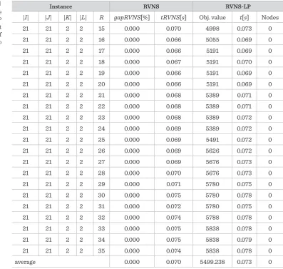
From the results presented in Table 1, it can be seen that for each instance from Data set 1, the solution obtained in RVNS phase coincides with the optimal one. The CPLEX solver that is employed within the LP part quickly proves its optimality, i.e., it is easily confirmed that the solution passed to CPLEX (and taken as a root node of Branch-and-Bound tree) is actually the optimal one. For this reason, in the case of the Data set 1, the number of nodes of the Branch-and-Bound tree generated during the CPLEX run is always equal to 0. The average CPU time of RVNS is 0.070 seconds, while the average CPU time of RVNS-LP is slightly longer – 0.073 seconds. Average gap of the RVNS solution is 0 %, meaning that the RVNS found optimal solution in each of the 20 runs.
Information Technology and Control 2017/1/46 108
Table 1
Results of the RVNS-LP for Data set 1 – the case of Montenegro
Instance RVNS RVNS-LP
|I| |J| |K| |L| R gapRVNS[%] tRVNS[s] Obj. value t[s] Nodes
21 21 2 2 15 0.000 0.070 4998 0.073 0
21 21 2 2 16 0.000 0.066 5055 0.069 0
21 21 2 2 17 0.000 0.066 5191 0.069 0
21 21 2 2 18 0.000 0.067 5191 0.070 0
21 21 2 2 19 0.000 0.066 5191 0.069 0
21 21 2 2 20 0.000 0.066 5191 0.069 0
21 21 2 2 21 0.000 0.068 5389 0.071 0
21 21 2 2 22 0.000 0.068 5389 0.071 0
21 21 2 2 23 0.000 0.068 5389 0.072 0
21 21 2 2 24 0.000 0.069 5389 0.072 0
21 21 2 2 25 0.000 0.069 5491 0.072 0
21 21 2 2 26 0.000 0.069 5626 0.072 0
21 21 2 2 27 0.000 0.069 5676 0.073 0
21 21 2 2 28 0.000 0.070 5676 0.073 0
21 21 2 2 29 0.000 0.071 5780 0.075 0
21 21 2 2 30 0.000 0.075 5780 0.078 0
21 21 2 2 31 0.000 0.072 5780 0.075 0
21 21 2 2 32 0.000 0.074 5788 0.078 0
21 21 2 2 33 0.000 0.075 5838 0.078 0
21 21 2 2 34 0.000 0.075 5838 0.079 0
21 21 2 2 35 0.000 0.074 5838 0.078 0
average 0.000 0.070 5499.238 0.073 0
showed to be the optimal one, since its optimality was quickly confirmed in the second phase by the LP method (the number of nodes is zero). The exception is the last instance with R = 40, where CPLEX solv-er has visited 7 nodes, starting from the best RVNS solution before finding the optimal solution. From the gapRVNS[%] column, it can be seen that the average
gap of RVNS solutions was 0.710 %, which means that some of the best solutions generated during 20 RVNS runs have small gaps from the optimal one. The aver-age time of the RVNS was 0.138 seconds through 20 runs, while RVNS-LP needed 0.157 seconds of run-ning time (in average) to return optimal solution. In order to analyze the quality of obtained solutions from practical point of view, we compare solutions obtained by the proposed model with the current
schedule of police units in Montenegro. The list of 21 municipalities in Montenegro is given in Table 3. The area of each municipality is observed as a location with a number assigned. In the present situation, all police units of type 2 are located in Podgorica, which is the capital of Montenegro, while police units of type 1 are located in municipalities 1, 3, 4, 5, 6, 12, 15, and 19, representing so-called security centers in Mon-tenegro. We have considered different combinations of parameter values b1, b2 and coverage radius R. For
Table 2
Results of the RVNS-LP for Data set 2 – the case of Serbia
Instance RVNS RVNS-LP
|I| |J| |K| |L| R gapRVNS[%] tRVNS[s] Obj. value t[s] Nodes
145 145 2 2 20 0.026 0.129 34638 0.138 0
145 145 2 2 21 0.250 0.126 34860 0.135 0
145 145 2 2 22 0.483 0.127 35997 0.136 0
145 145 2 2 23 0.210 0.131 37167 0.140 0
145 145 2 2 24 0.789 0.128 38019 0.137 0
145 145 2 2 25 0.642 0.132 38316 0.142 0
145 145 2 2 26 1.014 0.129 38451 0.138 0
145 145 2 2 27 0.898 0.131 38763 0.141 0
145 145 2 2 28 1.317 0.136 39168 0.147 0
145 145 2 2 29 0.894 0.134 39261 0.144 0
145 145 2 2 30 0.788 0.137 39999 0.147 0
145 145 2 2 31 0.446 0.139 40320 0.150 0
145 145 2 2 32 1.008 0.138 40776 0.149 0
145 145 2 2 33 1.400 0.143 40935 0.154 0
145 145 2 2 34 0.630 0.141 40977 0.153 0
145 145 2 2 35 0.674 0.143 41397 0.190 0
145 145 2 2 36 0.628 0.149 41553 0.172 1
145 145 2 2 37 0.898 0.148 41763 0.176 5
145 145 2 2 38 0.506 0.146 42111 0.171 0
145 145 2 2 39 0.704 0.152 42162 0.201 0
145 145 2 2 40 0.702 0.149 42285 0.226 7
average 0.710 0.138 39472.286 0.157 0.619
is given in Table 4. The number of police units of type 1 is fixed to 8, since all of them are located in security
Table 3
Municipalities in Montenegro
no. municip. no. municip. no. municip.
1 Podgorica 8 Žabljak 15 Plevlja
2 Andrijevica 9 Kolašin 16 Rožaje
3 Bar 10 Kotor 17 Tivat
4 Berane 11 Mojkovac 18 Ulcinj
5 Bijelo Polje 12 Nikšić 19 Herceg Novi
6 Budva 13 Plav 20 Cetinje
7 Danilovgrad 14 Plužine 21 Šavnik
centers. The number of units of type 2 that are cur-rently all located in Podgorica varies from 1 to 4, while covering radius R varies from 15 to 35 km.
Information Technology and Control 2017/1/46 110
Table 4
Comparisons of current locations and optimal locations of police units in Montenegro
Data Current solution Optimal solution
b1 b2 R locations of police units of type 1 locations of police units of type 2
Obj.
value locations of police units of type 1
locations of police units of type 2
Obj.
value Impr.[%]
8 1 15 1, 3, 4, 5, 6, 12 ,15, 19 1 3956 1, 3, 4, 6, 10, 12, 18, 19 13 4528 14.459
8 1 25 1, 3, 4, 5, 6, 12 ,15, 19 1 4727 1, 2, 3, 6, 12, 18, 19, 20 5 5207 10.154
8 1 35 1, 3, 4, 5, 6, 12 ,15, 19 1 5556 2, 3, 4, 6, 7, 9, 15, 19 14 5810 4.572
8 2 15 1, 3, 4, 5, 6, 12 ,15, 19 all in 1 3956 1, 3, 4, 6, 10, 12, 18, 19 5, 13 4638 17.240
8 2 25 1, 3, 4, 5, 6, 12 ,15, 19 all in 1 4727 1, 2, 3, 6, 12, 18, 19, 20 5, 15 5309 12.312
8 2 35 1, 3, 4, 5, 6, 12 ,15, 19 all in 1 5556 3, 4, 6, 7, 11, 13, 15, 19 8, 14 5825 4.842
8 3 15 1, 3, 4, 5, 6, 12 ,15, 19 all in 1 3956 1, 3, 4, 6, 10, 12, 18, 19 5, 13, 15 4740 19.818
8 3 25 1, 3, 4, 5, 6, 12 ,15, 19 all in 1 4727 1, 2, 3, 6, 12, 18, 19, 20 5, 15, 16 5397 14.174
8 3 35 1, 3, 4, 5, 6, 12 ,15, 19 all in 1 5556 2, 3, 4, 6, 7, 9, 15, 19 8, 14, 21 5838 5.076
8 4 15 1, 3, 4, 5, 6, 12 ,15, 19 all in 1 3956 1, 3, 4, 6, 10, 12, 18, 19 5, 13, 15, 16 4828 22.042
8 4 25 1, 3, 4, 5, 6, 12 ,15, 19 all in 1 4727 1, 2, 3, 6, 12, 18, 19, 20 5, 11, 15, 16 5459 15.486
8 4 35 1, 3, 4, 5, 6, 12 ,15, 19 all in 1 5556 2, 3, 4, 6, 7, 9, 15, 19 8, 12, 14, 21 5838 5.076
Figure 1
Current and optimal schedule of PSFUs for b1 = 8, b2 = 1 and R = 25
to 22.042 %. By analyzing the positions of police units in the current and optimal solution, we may notice the difference in locations of units of both types. For ex-ample, locations 2 (Andrijevica), 18 (Ulcinj) are often suggested by our model for establishing police units of type 1. For smaller values of covering radius R, location 10 (Kotor) is suggested, while for larger R, the model proposes location 15 (Pljevlja) for establishing police units of type 1. It is interesting that our model suggests relocation of police units of type 2, which are current-ly all situated at location 1 (Podgorica). For different values of b1, b2 and R, different locations are obtained;
however, locations 5 (Biljelo Polje) and 15 (Pljevlja) appear the most often. In Figure 1, we present current and optimal locations of police units for b1 = 8, b2 = 1,
and R = 25. Current locations of police units of types 1
and 2 are marked with blue digits, while locations in optimal solution are marked with red digits 1 and 2. The objective value of the solution corresponding to present situation is equal to 4727, while the objective value of the optimal solution provided by our model is 5207 (the improvement is around 10 %).
and security experts to improve the efficiency of po-lice system by relocating some popo-lice units. However, it is important to note that the decision where to lo-cate police units is not only driven by distances and statistical data on the number of criminal acts. In a real-life situation, it is important to take into account some additional conditions, such as the existence of adequate infrastructure, configuration of the terrain, possibility to observe larger geographical areas, etc. The decision making, including some of the men-tioned additional conditions, may be the subject of investigation in our future work.
Results on generated instances
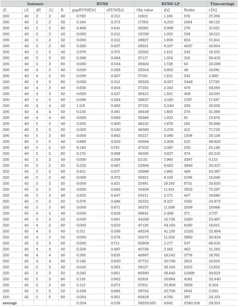
We have further benchmarked the RVNS-LP We have further benchmarked the RVNS-LP meth-od on generated instances from Data set 3, involving |I| = 200, 250 user nodes and |J| = 40, 45 potential lo-cations for emergency units. Differently from Data sets 1 and 2, in Data set 3, the number of incident types and the number of emergency unit types may be different, i.e., |K| ≠ |L| in general. The results are pre-sented in Table 5 in the same way as in Tables 1–2. In order to confirm that a good-quality RVNS solution that is passed as the initial solution to the LP method may significantly reduce the total running time, we add one more column ∆t[%] in Table 5. This column shows time savings (in percents) achieved by using the best RVNS solution from the first phase as the ini-tial solution in the LP phase.
From the results presented in Table 5, it can be seen that for larger problem instances with |I| = 200, 250 users, the RVNS phase produces high-quality solu-tions in short CPU times. The average running time of RVNS phase for instances in Table 5 is tRVNS = 0.536
seconds. The average gap of the objective value of the best solution produced by multi-start RVNS from the optimal one is low – 0.204 %, meaning that the best RVNS solution is close to the optimal one. Howev-er, the CPLEX solver applied within the LP part still needs additional effort to reach optimal solution starting from the best RVNS solution from the first phase, and to confirm its optimality. On average, the CPLEX solver visits 2340.104 nodes of the Branch-and-Bound tree until the optimal solution is found. The average running time that RVNS-LP needed to detect optimal solution and to confirm its optimality is quite short (9.641 seconds). Data presented in
col-umn ∆t[%] shows the advantage of the hybrid RVNS-LP method in respect to running times. Significant time savings (up to 75.597 %) are obtained when using solution from the RVNS phase as the initial solution for the CPLEX solver. In average, time savings are 29.353 % for instances from Table 5.
Information Technology and Control 2017/1/46 112
Instance RVNS RVNS-LP Time savings
|I| |J| |K| |L| R gapRVNS[%] tRVNS[s] Obj. value t[s] Nodes t [%]
200 40 2 2 40 0.760 0.313 15915 1.195 576 37.356
200 40 2 2 50 0.184 0.373 17363 4.232 1694 49.119
200 40 2 2 60 0.408 0.441 18383 0.999 276 31.621
200 40 3 2 40 0.000 0.312 24799 1.052 236 18.513
200 40 3 2 50 0.000 0.312 26937 1.606 654 31.841
200 40 3 2 60 0.280 0.437 28551 8.107 4037 18.954
200 40 3 3 40 0.578 0.375 25592 1.413 243 19.333
200 40 3 3 50 0.288 0.484 27117 1.334 318 58.432
200 40 3 3 60 0.000 0.544 28402 1.728 63 22.098
200 40 4 2 40 0.000 0.368 35504 0.855 49 19.081
200 40 4 2 50 0.000 0.407 37161 1.915 542 2.890
200 40 4 2 60 0.000 0.513 39329 9.307 3446 17.739
200 40 4 3 40 0.639 0.404 37255 2.163 479 59.565
200 40 4 3 50 0.000 0.437 38412 1.501 406 43.091
200 40 4 3 60 0.098 0.564 38827 4.160 1787 17.197
200 40 4 4 40 1.118 0.493 37133 2.240 339 19.339
200 40 4 4 50 0.216 0.591 38448 1.805 274 31.368
200 40 4 4 60 0.000 0.680 39386 1.933 91 13.474
200 40 5 3 40 0.305 0.460 48132 1.879 182 35.668
200 40 5 3 50 0.000 0.540 49380 2.276 412 71.720
200 40 5 3 60 0.000 0.662 50217 5.080 1208 20.126
200 40 5 5 40 0.869 0.502 45594 2.928 523 46.620
200 40 5 5 50 0.140 0.781 47233 3.097 250 55.148
200 40 5 5 60 0.179 0.688 48166 3.627 474 62.516
250 45 2 2 40 0.000 0.358 21151 7.963 3397 0.113
250 45 2 2 50 0.232 0.467 22884 9.482 3846 20.437
250 45 2 2 60 0.421 0.517 23990 1.865 499 54.387
250 45 3 2 40 0.000 0.372 30921 8.105 2196 15.949
250 45 3 2 50 0.000 0.431 33481 19.193 6731 35.620
250 45 3 2 60 0.000 0.482 35406 11.431 3832 75.597
250 45 3 3 40 0.535 0.447 34211 2.171 407 19.680
250 45 3 3 50 0.376 0.496 35332 9.327 1562 24.873
250 45 3 3 60 0.000 0.671 36370 11.098 2058 19.668
250 45 4 2 40 0.000 0.428 39841 2.499 371 3.737
250 45 4 2 50 0.000 0.491 44289 14.738 2580 23.487
250 45 4 2 60 0.000 0.622 47126 34.150 8190 19.915
250 45 4 3 40 0.311 0.509 48534 41.130 13181 22.894
250 45 4 3 50 0.000 0.579 50275 11.326 3882 20.424
250 45 4 3 60 0.000 0.711 50908 2.177 547 68.018
250 45 4 4 40 0.328 0.497 45739 3.162 463 31.283
250 45 4 4 50 0.395 0.635 46887 19.243 3778 18.765
250 45 4 4 60 0.149 0.820 47722 20.708 3915 19.833
250 45 5 3 40 0.043 0.563 58127 38.164 9353 13.853
250 45 5 3 50 0.345 0.661 60580 59.445 12499 30.623
250 45 5 3 60 0.118 0.802 61918 16.684 4183 32.440
250 45 5 5 40 0.112 0.673 57911 23.806 2858 8.354
250 45 5 5 50 0.328 0.865 59754 23.708 3041 2.053
250 45 5 5 60 0.054 0.951 60826 4.765 397 24.153
average 0.204 0.536 39529.563 9.641 2340.104 29.353
Table 5
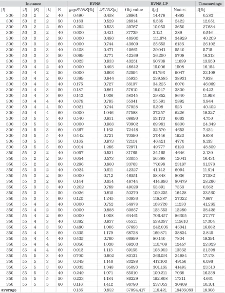
Table 6
Results of the RVNS-LP for Data set 3 – randomly generated large instances with |I| = 300 and |I| = 350 user nodes
Instance RVNS RVNS-LP Time savings
|I| |J| |K| |L| R gapRVNS[%] tRVNS[s] Obj. value t[s] Nodes t[%]
300 50 2 2 40 0.490 0.458 26961 14.478 4893 0.282
300 50 2 2 50 0.163 0.529 28914 8.585 2422 12.851
300 50 2 2 60 0.292 0.523 29767 10.953 3650 27.684
300 50 3 2 40 0.000 0.421 37739 2.121 289 0.516
300 50 3 2 50 0.000 0.496 40900 111.674 34929 40.209
300 50 3 2 60 0.000 0.744 43609 25.653 6136 26.102
300 50 3 3 40 0.408 0.471 40661 29.041 5540 5.715
300 50 3 3 50 0.099 0.771 42269 26.250 5708 16.313
300 50 3 3 60 0.023 0.933 43251 50.739 11699 13.550
300 50 4 2 40 0.000 0.493 48642 15.006 1508 16.154
300 50 4 2 50 0.000 0.603 52594 61.793 9047 32.108
300 50 4 2 60 0.399 0.844 55935 239.585 38931 7.838
300 50 4 3 40 0.175 0.727 56107 34.225 6070 46.069
300 50 4 3 50 0.187 0.861 57810 19.047 3800 0.422
300 50 4 3 60 0.142 1.036 58345 29.852 8640 11.998
300 50 4 4 40 0.679 0.795 55341 25.591 2892 3.944
300 50 4 4 50 0.021 0.744 57028 5.398 523 40.402
300 50 4 4 60 0.000 1.046 57588 37.257 6226 19.327
300 50 5 3 40 0.540 0.851 68690 53.170 6663 4.750
300 50 5 3 50 0.000 0.968 70902 69.981 8800 24.349
300 50 5 3 60 0.367 1.162 72448 32.570 4653 7.424
300 50 5 5 40 0.442 0.721 70590 27.446 1920 8.638
300 50 5 5 50 0.165 0.973 72114 46.421 4770 9.133
300 50 5 5 60 0.014 1.286 72971 49.777 6120 48.809
350 55 2 2 40 0.057 0.531 31765 24.165 4646 2.130
350 55 2 2 50 0.054 0.573 33055 56.398 12041 16.431
350 55 2 2 60 0.296 0.860 33763 77.698 23187 31.578
350 55 3 2 40 0.024 0.611 42327 41.142 6094 11.614
350 55 3 2 50 0.000 0.712 46551 58.848 8036 37.582
350 55 3 2 60 0.144 0.654 48744 414.896 80479 28.266
350 55 3 3 40 0.202 0.789 49029 53.891 7353 0.562
350 55 3 3 50 0.026 0.815 50270 109.235 16428 33.560
350 55 3 3 60 0.120 1.245 50936 118.387 27022 7.867
350 55 4 2 40 0.000 0.752 54878 108.720 11230 41.265
350 55 4 2 50 0.000 0.888 60857 123.553 12280 38.428
350 55 4 2 60 0.000 1.008 64461 706.457 86305 27.177
350 55 4 3 40 0.382 0.837 65511 538.097 115610 17.304
350 55 4 3 50 0.480 1.006 67693 242.005 45341 16.682
350 55 4 3 60 0.335 1.179 68728 169.871 38834 2.845
350 55 4 4 40 0.435 0.760 66899 80.140 7804 19.391
350 55 4 4 50 0.056 1.030 68203 110.708 12457 22.029
350 55 4 4 60 0.012 1.113 69155 108.952 13562 21.398
350 55 5 3 40 0.700 0.902 80131 266.091 24984 17.478
350 55 5 3 50 0.349 1.140 83288 417.100 49156 6.096
350 55 5 3 60 0.033 1.348 85093 301.165 41495 23.513
350 55 5 5 40 0.249 1.071 85010 100.211 7039 16.238
350 55 5 5 50 0.223 1.184 86229 192.808 17311 4.661
350 55 5 5 60 0.116 1.412 86780 237.053 30409 10.101
Information Technology and Control 2017/1/46 114
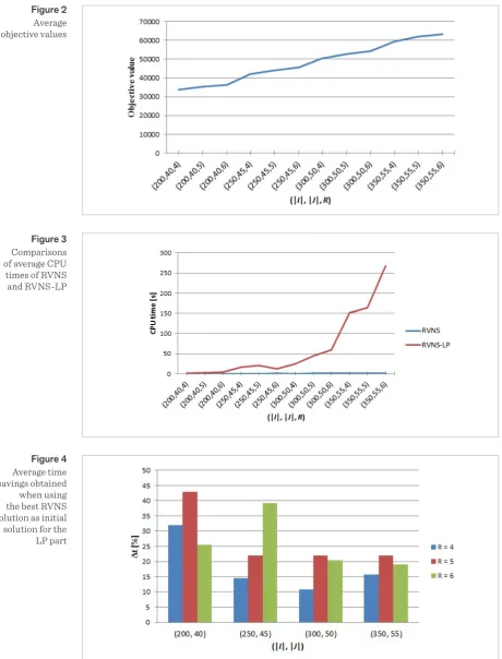
Figure 2
Average objective values
Figure 3
Comparisons of average CPU times of RVNS and RVNS-LP
Figure 4
Average time savings obtained when using the best RVNS solution as initial solution for the LP part
Figure 2. Average objective values
Figure 2. Average objective values
R = 60 is around 270 seconds, which is relatively short considering problem dimension and the fact that the optimal solution is provided. Finally, in Figure 4, we present the average time savings (in percents) obtained when using the best RVNS solution as the starting point for the LP part. Note that time-savings depend on the quality of the RVNS solution from the first phase as well as on the nature of the considered instances. As it can be seen in Figure 4, the average time-savings vary between 11 % an 43 % for the con-sidered groups of generated instances with fixed pa-rameters |I|, |J| and R.
Conclusions
This paper introduces the Multi-Type Maximal Cov-ering Location Problem (MTMCLP) in emergency service networks, representing a generalization of the well-known Maximal Covering Location Problem (MCLP). In the proposed MTMCLP, different types of incidents and emergency units are considered, and it is assumed that limited number of emergency units of each type is available. A hierarchy among emergency units is introduced, meaning that an emergency unit of a certain type can cover the same incident types as emergency units of lower level, as well as additional incident types. The objective of the MTMCLP is to find optimal locations for establishing emergency units of each type, so that the total sum of covered incidents is maximized. An efficient two-phase optimization algorithm (RVNS-LP) is designed to solve the con-sidered problem. In the first phase of the optimization algorithm, a variant of Reduced Variable Neighbor-hood Search (RVNS) is applied, producing high-qual-ity solution in very short CPU time. The RVNS uses neighborhood structures that are appropriate for the considered MTMCLP. The neighborhoods of the cur-rent solution are explored in an efficient manner by using a time-saving strategy in the procedure for ob-jective function calculation. The RVNS is run on the
set of randomly generated initial solutions, and the best solution obtained through multiple RVNS runs is used as the starting point for the Linear Program-ming method in the second phase. The LP method is used within the framework of commercial CPLEX software, and it was showed that significant savings of CPLEX running times may be obtained when using high-quality solution from the RVNS phase as the ini-tial solution for the LP part.
The proposed RVNS-LP was benchmarked on two sets of real-life instances and on the set of randomly generated instances of larger dimensions. Our exper-imental evaluation shown that the RVNS-LP solves all real-life instances to optimality in very short CPU times. On generated test instances, the RVNS-LP provided optimal solutions in reasonably short running times, having in mind problem dimensions. From practical point of view, solutions obtained by using the proposed model and RVNS-LP approach show significant improvement compared to current solutions regarding objective values, i.e., the increase of the total number of covered incidents. However, relocation of police units requires additional costs, but on the other side, it may lead to better efficiency of a security system. The solutions proposed in this study have a potential to be considered when creat-ing a long-term security system strategy. Future work may involve a modification of the proposed MTMCLP model in order to include some specific emergency system requirements, as well as adapting the RVNS-LP in order to solve similar covering problems relat-ed to emergency networks. The development of some metaheuristic methods for MTMCLP and testing their performances against the RVNS-LP is another future work direction.
Acknowledgement
This research was partially supported by Serbian Ministry of Education, Science and Technological Development under the grants nos. 174010, 044006, and 47017.
References
1. M. Abdolrazzagh-Nezhad, S. Abdullah. A Robust Intel-ligent Construction Procedure for Job-Shop Schedul-ing. Information Technology and Control, 2014, 43(3), 217–229. https://doi.org/10.5755/j01.itc.43.3.3536
Information Technology and Control 2017/1/46 116
3. O. Berman, D. Krass. The generalized maximal covering location problem. Computers and Operations Research, 2002, 29, 563–581. https://doi.org/10.1016/S0305-0548(01)00079-X
4. C. Blum, J. Puchinger, G. R. Raidl, A. Roli. Hybrid meta-heuristics in combinatorial optimization: A survey. Ap-plied Soft Computing, 2011, 11, 4135–4151. https://doi. org/10.1016/j.asoc.2011.02.032
5. R. L. Church, C. ReVelle. The maximal covering location problem. Papers of the Regional Science Association, 1974, 32, 101–118. https://doi.org/10.1007/BF01942293 6. R. L. Church. The planar maximal covering location
problem. Journal of Regional Science, 1984, 24(2), 185– 201. https://doi.org/10.1111/j.1467-9787.1984.tb01031.x 7. F. Colombo, R. Cordone, G. Lulli. The multimode cov-ering location problem. Computers and Operations Research, 2016, 67, 25–33. https://doi.org/10.1016/j. cor.2015.09.003
8. M. S. Daskin. Network and discrete location: Models, algorithms and applications. John Wiley & Sons: New York, US, 1995. https://doi.org/10.1002/9781118032343 9. Z. Drezner. The p-cover problem. European Journal of
Operational Research, 1986, 26, 312–313. https://doi. org/10.1016/0377-2217(86)90196-7
10. R. Z. Farahani, N. Asgari, N. Heidari, M. Hosseininia, M. Goh. Covering problems in facility location: A review. Computers & Industrial Engineering, 2012, 62(1), 368– 407. https://doi.org/10.1016/j.cie.2011.08.020
11. R. L. Francis, J. A. White. Facility layout and location an analytical approach (1st ed.). Prentice-Hall: Englewood Cliffs, NJ, USA, 1974.
12. P. Hansen, N. Mladenović. Variable neighborhood
search: Principles and applications. European Journal of Operational Research, 2001, 130, 449–467. https:// doi.org/10.1016/S0377-2217(00)00100-4
13. D. S. Hochbaum, A. Pathria. Analysis of the greedy ap-proach in the problems of maximum k-coverage. Na-val Research Logistics, 1998, 45, 615–627. https://doi. org/10.1002/(SICI)1520-6750(199809)45:6<615::AID-NAV5>3.0.CO;2-5
14. T. D. Klastorin. On the maximal covering location prob-lem and the generalized assignment probprob-lems. Man-agement Science, 1979, 25(1), 107–112. https://doi. org/10.1287/mnsc.25.1.107
15. A. Kolen, A. Tamir. Covering problems. In: P. Mirchan-dani, R. L. Francis (eds.), Discrete Location Theory, Wi-ley: New York, US, 1990, 263–304.
16. M. Marić, Z. Stanimirović, S. Božović. Hybrid
meta-heuristic method for determining locations for
long-term health care facilities. Annals of Operations Research, 2015, 227, 3–23. https://doi.org/10.1007/ s10479-013-1313-8
17. N. Megiddo, E. Zemel, S. L. Hakimi. The maximum coverage location problem. SIAM Journal of Algebraic and Discrete Methods, 1983, 4(2), 253–261. https://doi. org/10.1137/0604028
18. S. Mišković, Z. Stanimirović. A Memetic Algorithm
for Solving Two Variants of the Two-Stage Un-capacitated Facility Location Problem. Informa-tion Technology And Control, 2013, 42(2), 178–190. https://doi.org/10.5755/j01.itc.42.2.1768
19. N. Mladenovic´, P. Hansen. Variable neighborhood search. Computers Operations Research, 1997, 24, 1097–1100. https://doi.org/10.1016/S0305-0548(97)00031-2
20. S. Pirkwieser, G. R. Raidl, J. Puchinger. Combining Lagrangian decomposition with an evolutionary algo-rithm for the knapsack constrained maximum spanning tree problem. In: C. Cotta, J. I. van Hemert (eds.), Evolu-tionary Computation in Combinatorial Optimization, Springer: Berlin Heidelberg, 2007, 176–187. https://doi. org/10.1007/978-3-540-71615-0_16
21. C. ReVelle, J. Schweitzer, S. Snyder. The maximal con-ditional covering problem. INFOR, 1996, 34(2), 77–91. https://doi.org/10.1080/03155986.1996.11732294 22. G. R. Raidl, J. Puchinger, J. Combining (integer)
lin-ear programming techniques and metaheuristics for combinatorial optimization. In: C. Blum, M. J. B. Agu-ilera, A. Roli, M. Sampels (eds.), Hybrid Metaheuristics, Springer: Berlin, Heidelberg, 2008, 31–62. https://doi. org/10.1007/978-3-540-78295-7_2
23. C. ReVelle, K. Hogan. The maximum availability loca-tion problem. Transportaloca-tion Science, 1989, 23, 192– 200. https://doi.org/10.1287/trsc.23.3.192
24. D. A. Schilling, J. Vaidyanathan, R. Barkhi. A review of covering problems in facility location. Location Sci-ence, 1993, 1(1), 25–55.
25. Z. Stanimirović, I. Grujičić, D. Trifunović. Modeling the
Emergency Service Network of Police Special Forc-es Units for High-Risk Law Enforcement Operations. INFOR: Information Systems and Operational Re-search, 2014, 52(4), 206–226. https://doi.org/10.3138/ infor.52.4.206
26. P. Stanimirović, M. Marić, Z. Stanimirović. A
27. E. G. Talbi. Combining metaheuristics with mathemat-ical programming, constraint programming and ma-chine learning. 4OR, 2013, 11(2), 101–150.
28. C. D. T. Watson-Gandy. Heuristic procedures for the m-partial cover problem on a plane. European Journal
of Operation Research, 1982, 11, 149–157. https://doi. org/10.1016/0377-2217(82)90109-6
29. J. A. White, K. E. Case. On covering problems and the central facilities location problem. Geo-graphical Analysis, 1974, 6, 281–293. https://doi. org/10.1111/j.1538-4632.1974.tb00513.x
Summary / Santrauka
This study introduces the Multi-Type Maximal Covering Location Problem (MTMCLP) that arises from the design of emergency service networks, and represents a generalization of the well-known Maximal Covering Location Problem (MCLP). Differently from the basic MCLP, several types of incidents and emergency units are considered and hierarchy of emergency units of different types is assumed in the MTMCLP. The numbers of available emergency units of each type are limited to some constants. The objective of the MTMCLP is to choose locations for establishing emergency units of each type, such that the total number of covered incidents is maximized. In order to provide a decision maker with optimal solutions in an efficient manner, a two-phase optimization approach to the MTMCLP is designed. In the first phase, a variant of Reduced Variable Neigh-borhood Search (RVNS) is applied to quickly find a high-quality solution. The obtained RVNS solution is used as a good starting point for the Linear Programming method in the second phase, which returns the optimal solution to the MTMCLP. All constructive elements of the proposed two-phase method, denoted as RVNS-LP, are adapted to the characteristics of the considered problem. The RVNS-LP approach is evaluated on real-life instances obtained from two networks of police units in Montenegro and Serbia, and randomly generated test instances of larger dimensions. Experimental evaluation shows that the proposed RVNS-LP reached all opti-mal solutions on all real-life test instances in very short CPU time. On generated test instances, the RVNS-LP also returned optimal solutions in all cases, within short running times and significant time savings compared to CPLEX solver. The mathematical model and the proposed two-phase optimization method may be applicable in the design and management of various emergency-service networks.