A Time-Constrained Algorithm for Integration Testing in a Data Warehouse Environment

(1)

5

Information Technology and Control 2018/1/47

A Time-Constrained Algorithm

for Integration Testing in a Data

Warehouse Environment

ITC 1/47

Journal of Information Technology and Control

Vol. 47 / No. 1 / 2018 pp. 5-25

DOI 10.5755/j01.itc.47.1.18171 © Kaunas University of Technology

A Time-Constrained Algorithm for Integration Testing in a Data Warehouse Environment

Received 2017/05/11 Accepted after revision 2018/01/22

http://dx.doi.org/10.5755/j01.itc.47.1.18171

Corresponding author: [email protected]

Ljiljana Brkić, Igor Mekterović

University of Zagreb, Faculty of Electrical Engineering and Computing, Unska 3, 10000 Zagreb, Croatia, e-mail: [email protected], [email protected]

A data warehouse should be tested for data quality on regular basis, preferably as a part of each ETL cycle. That way, a certain degree of confidence in the data warehouse reports can be achieved, and it is generally more likely to timely correct potential data errors. In this paper, we present an algorithm primarily intended for integration testing in the data warehouse environment, though more widely applicable. It is a generic, time-constrained, metadata driven algorithm that compares large database tables in order to attain the best global overview of the data set’s differences in a given time frame. When there is not enough time available, the algorithm is capable of producing coarse, less precise estimates of all data sets differences, and if allowed enough time, the algorithm will pinpoint exact differences. This paper presents the algorithm in detail, presents algorithm evaluation on the data of a real project and TPC-H data set, and comments on its usability. The tests show that the algorithm outperforms the relational engine when the percentage of differences in the database is relatively small, which is typical for data warehouse ETL environments.

KEYWORDS: Data Warehouse Testing, ETL, Integration Testing, Data Quality.

1. Introduction

Data quality is a key factor in data warehouse (DW) and business intelligence solutions. Continuous test-ing of a DW can provide a solid assessment of the data quality. DW testing process should be implemented at very early stages of DW system development, leading to early error detection and correction which will, in

turn, increase DW’s credibility and decrease opera-tional costs in the long run.

(2)

at-Information Technology and Control 2018/1/47 6

tributes [38]. These attributes are called data quality dimensions. Each dimension covers a specific aspect of quality. For quantitative assessment of quality di-mensions, it is necessary to define metrics and mea-surement methods. Researchers have recognized the importance of this issue and many research papers (some of which are [13], [18], [21], [30], [38]) deal with methods of measuring or quantifying dimensions of data quality.

Apart from the source data, the quality of DW data is also affected by the ETL process used to integrate and transfer the data. Faulty ETL process, whether be-cause of the faulty logic, inappropriate data refresh-ment strategy or just plain programming errors, can cause data not to be transferred to the DW or not to be transferred in a timely fashion. With that in mind, it is important to assess how accurate and complete data are: whether all required data from the data sources are extracted, stored in the staging area, transformed and subsequently loaded into the DW and whether the data in the DW are accurate with regards to the source data. We adopt the accuracy definition from [3] “Accuracy is defined as the closeness between a value v and a value v’, considered as the correct rep-resentation of the real-life phenomenon that v aims to represent” and completeness definition from [2]: “Presence of all defined content at both data element and data set levels.” The assessment of accuracy and completeness of the data in a DW imposes comparing large data sets which is at the core of the DW’s inte-gration testing [24].

This paper is concerned with those very issues – we present an algorithm for integration testing of accu-racy and completeness of the DW data in the sense of the aforementioned definitions. Integration testing is an approach to software testing where software components are combined and tested as a group, with the purpose of ensuring that interacting components or subsystems interface correctly with one another. Integration testing in DW environment usually only includes testing the ETL application, which compris-es of numerous packagcompris-es. ETL packagcompris-es are tcompris-ested by examining data at the endpoints (input and output) of those packages. In DW environment, we can identify three typical subsystems that ETL application deals with: data source(s), data staging area and DW pro-duction tables (typically dimension and fact tables). We perform integration testing by comparing

vari-ous corresponding data sets from those three sourc-es using the proposed TCFC (Time-Constrained Fragment and Compare) algorithm. The algorithm is generic and widely applicable, not limited to DW en-vironment. It provides an overview of the differenc-es between two data sets depending on the assigned time frame, from performing shallow comparisons to pinpointing exact differing tuples. We present the algorithm in detail, comment on its features, evaluate it on data of a real project as well as on mock data and comment on the results.

2. Motivation

The primary objective of the integration testing and TCFC algorithm presented in this paper is to get a global overview of the data quality in the DW with a focus on accuracy and completeness measures. These measures are considered with respect to the source systems, as we assume that the data in the source sys-tem are accurate and complete. In this generic test in-tegration scenario, involving source, staging and DW subsystems, testing should provide answers to the following questions:

a whether all required data from the data sources been extracted and transferred to the staging area (completeness), and whether staging area attri-bute values are equal to corresponding values in source systems (accuracy);

b whether all required data from the staging area been transferred to the DW (completeness), and whether corresponding attribute values are equal (accuracy).

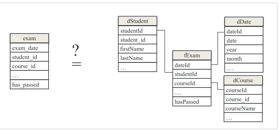
To answer the first question, the data from the data sources must be compared to the data stored in the staging area, where they are stored in the identical or similar schemas. To answer the second question, data from the staging area must be compared to the data in the DW, where they may be stored in different (though mappable) structures, e.g., dimensional mod-el. In both cases, the problem boils down to comparing two sets of database tables having identical or differ-ent but mappable schemas to find missing or excess tuples on either side, and/or matching tuples with dif-ferent values of non-key attributes.

(3)

7

to that problem, since they are highly optimized for set operations on data: Two tables can be compared for differences with a single SQL statement. This approach, however, which will be referred to as ref-erence implementation hereafter, has two serious drawbacks that motivated our research:

3 It is not possible to span a single SQL query across heterogeneous platforms. That is a common sce-nario in DW environment, especially between source systems and staging area. To compare ta-bles from different environments, table from one server would have to be transferred to a (tempo-rary) table on the other server or some sort of da-tabase integration software would have to be used that would abstract that operation. Either way, the very operation of moving the data from one DBMS to another is subject to error. Transfer errors can occur for various reasons. For instance, IBM Infor-mix’s DATE type has a wider DATE range than SQL Server’s, and rows with such dates simply cannot be inserted into the SQL Server table having the exact same schema.

4 It is an all-or-nothing approach. It is not possible to perform a “shallow comparison” – a compar-ison that would take much less time to execute but would not be completely accurate (i.e. detect all differences in all tables) and/or precise (i.e. pinpoint the exact tuples causing differences). All rows from one table are compared to all rows from the other table and in the case when there is a substantial number of rows (tens of millions and more), such a comparison can also take a substan-tial resources to execute. A large table comparison could block all others and take up all available time. In other words, such queries cannot be appropri-ately time-managed to fit into a given time frame. Time managing queries is very important because testing procedures have to fit into the ETL’s ac-ceptable time frame. It is unacac-ceptable to query the data sources at arbitrary times, inflicting addition-al burden on the production systems.

Sometimes, when comparing two tables via a sin-gle SQL statement, it is handy to use a hash function (e.g., MD5) to produce the checksum of the tuple. This shortens the SQL statement, but, in general, calcu-lating checksums additionally slows the comparison and is not suitable for large data sets, especially if checksums cannot be stored (e.g., ETL has read only

access to source systems). Checksums are applicable to TCFC with similar properties, as commented in Section 3.1.

In terms of complexity, comparing two data sets is O(n2_{) complex, where every record from the first set} has to be compared with records from the second set. Another valid approach, used by some commercial tools (e.g., SQL Data Examiner [35]), is to fetch re-cords sorted by the primary key from the databases and perform a less complex merge-sort style compari-son; however – it must be taken into account that sort-ing data at the sources incurs additional costs. Both approaches suffer from the 2nd_{drawback described} above: they are prone to blocking the entire compari-son when large tables are examined. In addition, such approaches rely heavily on the client’s resources (disk and memory) as both sets must be retrieved in their entirety. Time-managing testing (queries) is what makes this problem difficult, and, to the best of our knowledge, has not been addressed in the literature so far (see the section “Related Work” for more). This motivated us to develop an algorithm that will surpass these limitations, yet remain comparable to the reference implementation in terms of speed. Since the expected number of differences between the tables is relatively small when compared to the to-tal number of rows, we formulate the TCFC algorithm requirements as follows:

_ When applied to large data sets with a small number of differences, the algorithm should be comparable in terms of speed with the reference implementation. One could argue that having 10k or 100k faulty tuples is “the same” because such a large number of errors is either a sign of systemic error or an unmanageable number of data errors that cannot be manually corrected. Therefore, the algorithm should work well for a manageable number of differing rows, hundreds or thousands of errors, not millions.

_ Must be suitable for comparing data across heterogeneous platforms.

_ Must be time manageable, to fit into a configured time frame, at the expense of precision. In other words, it must be able to perform “shallow comparisons” and, consequently, has to be configurable.

(4)

break-Information Technology and Control 2018/1/47 8

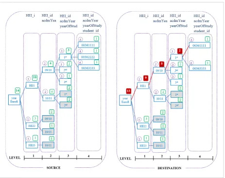
ing down the exhausting reference query into many faster queries that search for potential errors in a greedy fashion. This is done by subsequently break-ing data into horizontal fragments and comparbreak-ing fragment counts (and/or other aggregated values) of corresponding fragments. As the algorithm progress-es, fragmentation filters are refined, so that the frag-ments become smaller. Fragfrag-ments where inequali-ties are detected are examined with higher priority. Eventually, if so configured and if time allows it, the comparison could be brought to the primary key level, thus yielding the exact missing or excess tuples. When designing the TCFC algorithm, we were guided by the thought that, given a limited time, it is better to acquire a possibly not completely accurate overview

of all tables rather than an accurate comparison of

some tables, while leaving others not examined. We denote this approach as “good enough global over-view”. In other words, if there is a large set of table pairs with only several containing differences, it is considered better to report that there are some

differ-ences in all of the pairs actually containing

differenc-es, than to pinpoint exact differences in just a few of them, and leave the rest of the tables unexamined. It is a position that we have attained after participating in few real world projects and, though it might not be the best strategy for all applications, we believe that it is the best one in the most of DW ETL scenarios.

3. TCFC Algorithm

The TCFC algorithm is designed to be as generic as possible and to work on heterogeneous platforms and with large data sets. To apply the proposed algorithm to a DW, the following conditions must be met: _ Data sources are relational databases, since the

algorithm leverages relational engine. Other sources of data (text files, spreadsheets or other office documents, XML files, etc.) are not supported. As a workaround to this limitation, data from other sources can be processed and stored in a relational database (“piped through”).

_ Each record in the destination table corresponds to exactly one record in the source table. This requirement can be worked around by adding an additional metadata layer to describe the acceptable differences. For instance, with slowly

changing dimensions, the number of regular “duplicates” can be kept. Furthermore, a generic system of human reviewing and (dis)approving differences could be put in place, where an analyst would mark the correct differing tuples and they would be taken into account in the future comparisons. We do not describe such system in more detail here, though. As a side note, our real-world project use-case required for a 100% match between the source and DW (students’ exams, year and course enrollments, etc.).

_ Data lineage [4-5] must be established, there must be a way to determine the source for each tuple in data warehouse tables. To do so, it might be necessary to make minor modifications to existing ETL procedures. The procedure for establishing data lineage in existing systems, which is used in this paper, is described in detail in [26].

In the following two sections, we formally describe the table-level part of the TCFC algorithm for com-paring tables with identical and non-identical sche-mas, then present the overall algorithm in a pseudo code, provide a running example, present and discuss the performance testing and the associated results. 3.1. Determining Inequalities in the Content of Tables Having Identical Schemas

.

The algorithm works by fragmenting tables accord-ing to a fragmentation set, then one or more aggre-gate functions are evaluated upon each fragment, and finally, the results from the corresponding fragments are compared. Any differences, if found, indicate not only that the contents of � and � are different, but also point out to the group of tuples, i.e. fragment of the relation to which the problem pertains. What follows is a formal description of the stated.

Let � and � be the tables (relations) having the sche-ma �. Let � denote a relation with schema � = {��, … , ��}. Domain for attribute � is denoted by ��(�). Let � be a (possibly empty) subset of �. Let � denote a tuple. Let �� denote an X-value of �, i.e. tuple � restricted to �.

Let ℰ(�, �) denote the equivalence relation on � de-rived from equivalency of tuple’s X-values. We say that tuples ��, ��∈ � are equivalent under ℰ(�, �) iff the tuples have equal X-values, i.e. (��, ��) ∈ ℰ(�, �) � �� = ��. It should be noted that if � = � then �� = �� for each (��, ��) ∈ �, ren-dering all tuples in � equivalent under ℰ(�, �). Different X-values of � correspond with X-values of tuples in ��(�) (projection on the attributes con-tained in �). Each tuple � ∈ ��(�) unambiguously identifies an equivalence class, i.e. fragment ℱ(�, �, �) = {� ∈ � | �� = �}.

Consequently, equivalence relation ℰ(�, �) partitions relation � into the set of fragments ℱ(�, �) = {ℱ(�, �, �) | � ∈ ��(�)}. Because the set � deter-mines the fragmentation strategy of the �, hereinaf-ter we will refer to the set � as to the fragmentation set. In the specific case when fragmentation set � is empty, ��(�) produces a single-tuple zero-degree relation, with the effect that ℰ(�, �) partitions � into exactly one fragment which is equal to �.

Let �ℱ be the set of available aggregate functions, where �� denotes an aggregate function (e.g., count, sum, max, min). Let ℬ be the set of arbitrary attribute names ��, ��, …, subjected to the constraint that none of the attribute names appears in �. Relation ��,� is a set of triplets (��, �, �) which relates ag-gregate functions from �ℱ, attributes from � � � and attribute names from ℬ in the following way: if (��, �, �) ∈ ��,�, then aggregate function �� is evaluated for attribute � and the result is named �. Henceforth, we will refer to the relation ��,� as the aggregation set.

Aggregate function �� must be applicable to the do-main of the attribute �. More than one aggregate function �� can be applied upon each attribute � and each � ∈ ℬ appears exactly in one triplet. Formally, ��,�= {(��, �, �) | (��, �, �) ∈ �ℱ × (� � �) ×

ℬ � �� (�)} ∀(��, ��, ��), ��, ��, �� ∈ ��,�� = ��

� ��= �� = ��

Designated aggregate functions from ��,� are ap-plied upon fragment ℱ(�, �, �), the results of aggre-gate functions are renamed and concatenated to tu-ple �. The overall result of the operation is a single-tuple relation ��, �, ��,�, �� with schema

� � {��, ��, … ��}, where � = ��,��: ��, �, ��,�, �� = � � ��(�)

��{��(�) | (��, A,�)∈ ��,�}ℱ(�, �, �)�.

Applying the aggregate functions upon each frag-ment, ℱ(�, �, �) ∈ ℱ(�, �) would yield a set of rela-tions ��, �, ��,�, ��, exactly one relation per each � ∈ ��(�). Union of these relations, denoted as ��, �, ��,��, can be effectively evaluated with rela-tional algebra grouping operator:

��, �, ��,�� = ⋃�∈��(�)��, �, ��,�, ��= ��(�)� �� {��(�) | (��, A,�)∈ ��,�}��.

Given the relation schema �, relations �(�) and �(�), beforehand determined sets � and ��,�, one can eas-ily evaluate ��, �, ��,�� and ��, �, ��,��.

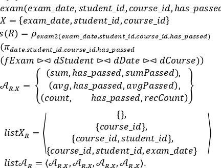
For instance, only consider the relation “exam” in the left part of the Figure1, and suppose that we want to compare it with the identical-schema relation in an-other database. One possible fragmentation setup could be:

r(R)=exam(exam_date, student_id, course_id, has_passed)

s(R)=exam(exam_date, student_id, course_id, has_passed)

X={exam_date,student_id,course_id}

��,�= �

(��, ��, ��), (��, ��, ��),

(��, ��, ��)�.

(5)

9

.

Let � and � be the tables (relations) having the sche-ma �. Let � denote a relation with schema � = {��, … , ��}. Domain for attribute � is denoted by ��(�). Let � be a (possibly empty) subset of �. Let � denote a tuple. Let �� denote an X-value of �, i.e. tuple � restricted to �.

Let ℰ(�, �) denote the equivalence relation on � de-rived from equivalency of tuple’s X-values. We say that tuples ��, ��∈ � are equivalent under ℰ(�, �) iff the tuples have equal X-values, i.e. (��, ��) ∈ ℰ(�, �) � �� = ��. It should be noted that if � = � then �� = �� for each (��, ��) ∈ �, ren-dering all tuples in � equivalent under ℰ(�, �). Different X-values of � correspond with X-values of tuples in ��(�) (projection on the attributes con-tained in �). Each tuple � ∈ ��(�) unambiguously identifies an equivalence class, i.e. fragment ℱ(�, �, �) = {� ∈ � | �� = �}.

Consequently, equivalence relation ℰ(�, �) partitions relation � into the set of fragments ℱ(�, �) = {ℱ(�, �, �) | � ∈ ��(�)}. Because the set � deter-mines the fragmentation strategy of the �, hereinaf-ter we will refer to the set � as to the fragmentation set. In the specific case when fragmentation set � is empty, ��(�) produces a single-tuple zero-degree relation, with the effect that ℰ(�, �) partitions � into exactly one fragment which is equal to �.

Let �ℱ be the set of available aggregate functions, where �� denotes an aggregate function (e.g., count, sum, max, min). Let ℬ be the set of arbitrary attribute names ��, ��, …, subjected to the constraint that none of the attribute names appears in �. Relation ��,� is a set of triplets (��, �, �) which relates ag-gregate functions from �ℱ, attributes from � � � and attribute names from ℬ in the following way: if (��, �, �) ∈ ��,�, then aggregate function �� is evaluated for attribute � and the result is named �. Henceforth, we will refer to the relation ��,� as the aggregation set.

Aggregate function �� must be applicable to the do-main of the attribute �. More than one aggregate function �� can be applied upon each attribute � and each � ∈ ℬ appears exactly in one triplet. Formally, ��,�= {(��, �, �) | (��, �, �) ∈ �ℱ × (� � �) ×

ℬ � �� (�)} ∀(��, ��, ��), ��, ��, �� ∈ ��,�� = ��

� ��= �� = ��

Designated aggregate functions from ��,� are ap-plied upon fragment ℱ(�, �, �), the results of aggre-gate functions are renamed and concatenated to tu-ple �. The overall result of the operation is a single-tuple relation ��, �, ��,�, �� with schema

� � {��, ��, … ��}, where � = ��,��: ��, �, ��,�, �� = � � ��(�)

��{��(�) | (��, A,�)∈ ��,�}ℱ(�, �, �)�.

Applying the aggregate functions upon each frag-ment, ℱ(�, �, �) ∈ ℱ(�, �) would yield a set of rela-tions ��, �, ��,�, ��, exactly one relation per each � ∈ ��(�). Union of these relations, denoted as ��, �, ��,��, can be effectively evaluated with rela-tional algebra grouping operator:

��, �, ��,�� = ⋃�∈��(�)��, �, ��,�, ��= ��(�)� �� {��(�) | (��, A,�)∈ ��,�}��.

Given the relation schema �, relations �(�) and �(�), beforehand determined sets � and ��,�, one can eas-ily evaluate ��, �, ��,�� and ��, �, ��,��.

s(R)=exam(exam_date, student_id, course_id, has_passed) X={exam_date,student_id,course_id} ��,�= � (��, ��, ��), (��, ��, ��), (��, ��, ��)�.

Tuples ��∈ ��, �, ��,�� and ��∈ ��, �, ��,��, where �� = �� = � contain the results of aggre-gate functions applied on fragments ℱ(�, �, �) and ℱ(�, �, �), respectively. The inequality of the tuples implies the difference between the corresponding fragments, i.e. ��≠ ��⇒ ℱ(�, �, �) ≠ ℱ(�, �, �), .

Let � and � be the tables (relations) having the sche-ma �. Let � denote a relation with schema � =

{��, … , ��}. Domain for attribute � is denoted by

��(�). Let � be a (possibly empty) subset of �. Let � denote a tuple. Let �� denote an X-value of �, i.e. tuple � restricted to �.

Let ℰ(�, �) denote the equivalence relation on �

de-rived from equivalency of tuple’s X-values. We say that tuples ��, ��∈ � are equivalent under ℰ(�, �) iff

the tuples have equal X-values, i.e. (��, ��) ∈

ℰ(�, �) � �� = ��. It should be noted that if

� = � then �� = �� for each (��, ��) ∈ �,

ren-dering all tuples in � equivalent under ℰ(�, �). Different X-values of � correspond with X-values of tuples in ��(�) (projection on the attributes

con-tained in �). Each tuple � ∈ ��(�) unambiguously

identifies an equivalence class, i.e. fragment

ℱ(�, �, �) = {� ∈ � | �� = �}.

Consequently, equivalence relation ℰ(�, �) partitions relation � into the set of fragments ℱ(�, �) =

{ℱ(�, �, �) | � ∈ ��(�)}. Because the set �

deter-mines the fragmentation strategy of the �, hereinaf-ter we will refer to the set � as to the fragmentation set. In the specific case when fragmentation set � is empty, ��(�) produces a single-tuple zero-degree

relation, with the effect that ℰ(�, �) partitions � into exactly one fragment which is equal to �.

Let �ℱ be the set of available aggregate functions, where �� denotes an aggregate function (e.g., count, sum, max, min). Let ℬ be the set of arbitrary attribute names ��, ��, …, subjected to the constraint that

none of the attribute names appears in �. Relation ��,� is a set of triplets (��, �, �) which relates

ag-gregate functions from �ℱ, attributes from � � � and attribute names from ℬ in the following way: if

(��, �, �) ∈ ��,�, then aggregate function �� is

evaluated for attribute � and the result is named �. Henceforth, we will refer to the relation �_�,� as the aggregation set.

Aggregate function �� must be applicable to the do-main of the attribute �. More than one aggregate function �� can be applied upon each attribute � and each � ∈ ℬ appears exactly in one triplet. Formally,

��,�= {(��, �, �) | (��, �, �) ∈ �ℱ × (� � �) ×

ℬ � �� (�)}

∀(��, ��, ��), ��, ��, �� ∈ ��,�� = ��

� ��= �� = ��

Designated aggregate functions from ��,� are

ap-plied upon fragment ℱ(�, �, �), the results of aggre-gate functions are renamed and concatenated to tu-ple �. The overall result of the operation is a single-tuple relation ��, �, ��,�, �� with schema

� � {��, ��, … ��}, where � = ��,��:

��, �, ��,�, �� = � � ��(�)

��{��(�) | (��, A,�)∈ ��,�}ℱ(�, �, �)�.

Applying the aggregate functions upon each frag-ment, ℱ(�, �, �) ∈ ℱ(�, �) would yield a set of rela-tions ��, �, ��,�, ��, exactly one relation per each

� ∈ ��(�). Union of these relations, denoted as

��, �, ��,��, can be effectively evaluated with

rela-tional algebra grouping operator:

��, �, ��,�� = ⋃�∈��(�)��, �, ��,�, ��=

��(�)� �� {��(�) | (��, A,�)∈ ��,�}��.

Given the relation schema �, relations �(�) and �(�), beforehand determined sets � and �_�,�, one can eas-ily evaluate ��, �, ��,�� and ��, �, ��,��.

Tuples ��∈ ��, �, ��,�� and ��∈ ��, �, ��,��,

where �� = �� = � contain the results of

aggre-gate functions applied on fragments ℱ(�, �, �) and ℱ(�, �, �), respectively. The inequality of the tuples implies the difference between the corresponding fragments, i.e. ��≠ ��⇒ ℱ(�, �, �) ≠ ℱ(�, �, �),

.

Let � and � be the tables (relations) having the sche-ma �. Let � denote a relation with schema � =

{��, … , ��}. Domain for attribute � is denoted by

��(�). Let � be a (possibly empty) subset of �. Let � denote a tuple. Let �� denote an X-value of �, i.e. tuple � restricted to �.

Let ℰ(�, �) denote the equivalence relation on �

de-rived from equivalency of tuple’s X-values. We say that tuples ��, ��∈ � are equivalent under ℰ(�, �) iff

the tuples have equal X-values, i.e. (��, ��) ∈

ℰ(�, �) � �� = ��. It should be noted that if

� = � then �� = �� for each (��, ��) ∈ �,

ren-dering all tuples in � equivalent under ℰ(�, �). Different X-values of � correspond with X-values of tuples in ��(�) (projection on the attributes

con-tained in �). Each tuple � ∈ ��(�) unambiguously

identifies an equivalence class, i.e. fragment ℱ(�, �, �) = {� ∈ � | �� = �}.

Consequently, equivalence relation ℰ(�, �) partitions relation � into the set of fragments ℱ(�, �) =

{ℱ(�, �, �) | � ∈ ��(�)}. Because the set �

deter-mines the fragmentation strategy of the �, hereinaf-ter we will refer to the set � as to the fragmentation set. In the specific case when fragmentation set � is empty, ��(�) produces a single-tuple zero-degree

relation, with the effect that ℰ(�, �) partitions � into exactly one fragment which is equal to �.

Let �ℱ be the set of available aggregate functions,

where �� denotes an aggregate function (e.g., count, sum, max, min). Let ℬ be the set of arbitrary attribute names ��, ��, …, subjected to the constraint that

none of the attribute names appears in �. Relation ��,� is a set of triplets (��, �, �) which relates

ag-gregate functions from �ℱ, attributes from � � � and attribute names from ℬ in the following way: if

(��, �, �) ∈ ��,�, then aggregate function �� is

evaluated for attribute � and the result is named �. Henceforth, we will refer to the relation ��,� as the

aggregation set.

Aggregate function �� must be applicable to the do-main of the attribute �. More than one aggregate function �� can be applied upon each attribute � and each � ∈ ℬ appears exactly in one triplet. Formally,

��,�= {(��, �, �) | (��, �, �) ∈ �ℱ × (� � �) ×

ℬ � �� (�)}

∀(��, ��, ��), ��, ��, �� ∈ ��,�� = ��

� ��= �� = ��

Designated aggregate functions from ��,� are

ap-plied upon fragment ℱ(�, �, �), the results of aggre-gate functions are renamed and concatenated to tu-ple �. The overall result of the operation is a single-tuple relation ��, �, �_�,�, �� with schema

� � {��, ��, … ��}, where � = ��,��:

��, �, ��,�, �� = � � ��(�)

��{��(�) | (��, A,�)∈ ��,�}ℱ(�, �, �)�.

Applying the aggregate functions upon each frag-ment, ℱ(�, �, �) ∈ ℱ(�, �) would yield a set of rela-tions ��, �, ��,�, ��, exactly one relation per each

� ∈ ��(�). Union of these relations, denoted as

��, �, ��,��, can be effectively evaluated with

rela-tional algebra grouping operator:

��, �, ��,�� = ⋃�∈��(�)��, �, ��,�, ��=

��(�)� �� {��(�) | (��, A,�)∈ ��,�}��.

Given the relation schema �, relations �(�) and �(�), beforehand determined sets � and ��,�, one can

eas-ily evaluate ��, �, ��,�� and ��, �, ��,��.

Tuples ��∈ ��, �, ��,�� and ��∈ ��, �, ��,��,

where �_�� = �� = � contain the results of

aggre-gate functions applied on fragments ℱ(�, �, �) and ℱ(�, �, �), respectively. The inequality of the tuples implies the difference between the corresponding fragments, i.e. ��≠ ��⇒ ℱ(�, �, �) ≠ ℱ(�, �, �),

which leads to the conclusion that ��

�� .

Actually, any difference between �� and

�� implies the inequality of � and �.

Unfor-tunately, the inverse is not true, i.e. even when

�� = �� , it is still possible that �

and � are not equal. This happens in very rare cases when differences of attribute values cumulatively nullify each other during aggregate function evalua-tion [26]. Opportunely, already low probability of such an event can be further reduced to the accepta-ble level by applying larger set of aggregate functions. This is the reason why the equiva-lence �� = �� = �, alt-hough not strictly correct, will be considered as ade-quate for practical purpose of comparing fragments. As a side note, an interesting approach that would also almost guarantee the equivalence would be to use a single aggregate function that aggregates tuple hashes. Such an aggregate function should be com-mutative, because ordering tuples would incur addi-tional costs. For instance, SQL Server provides CHECKSUM_AGG function (which, though undoc-umented, we suspect is a simple XOR function) that can be used to that purpose. Similar remarks apply here as for the reference implementation – this is not suitable for large tables because calculating hashes on the fly is costly, and storing and maintaining addi-tional hash data is often not possible, especially at source data systems.

The reason why the aggregate functions are applied only upon attributes in � � � is straightforward. Ap-plying aggregate functions upon an attribute from � would be unproductive because X-values of tuples in corresponding fragments of � and � are identical by definition, so are the results of aggregate functions. The number of fragments in ℱ(�� ) depends on the contents of the fragmentation set �. Generally, in-creasing the cardinality of �, increases the cardinali-ty of ��(�), which in turn increases the number of tuples in �� , hence decreasing the average number of tuples per fragment. There is a trade-off in selection of attributes for the fragmentation set �. Using larger fragmentation set provides more precise determination of relation’s subset which is the source of differences, but simultaneously degrades the performance due to increased number of groups for which aggregate functions have to be evaluated and their results compared. On the other hand, the contents of the aggregation set �� do not signifi-cantly affect the performance, because the cost of aggregate function evaluation is negligible compared

with the cost of grouping operation. Obviously, the main issue is to appropriately determine the content of the fragmentation set. The two extreme cases are: to use empty fragmentation set, which will produce exactly one fragment, or, to use one of the keys or superkeys for �, which will produce altogether

��(�) single-tuple fragments.

Taking into account the aforementioned trade-off and presuming that only a relatively small number of pairs of relations is expected to be actually different, we concluded that the process of comparing rela-tions should start with the empty or nearly empty fragmentation set ��. If �� =

�� , then the pair can be left out of further

inspection. Otherwise, in order to determine the group of tuples incurring differences more precisely, procedure can be iteratively carried out. In each step of the procedure, fragmentation set is augmented with additional attributes, thus increasing the num-ber of fragments and decreasing the fragment’s tuple count. The process is repeated until maximal frag-mentation set (with all intended attributes) has been inspected or allotted time frame has expired.

In order to carry out the described procedure, the following information has to be defined (and stored in a metadata repository) for each pair of relations r(R) and s(R):

1. Nonempty list of fragmentation sets, denoted as

��:

��= 〈�� 〉,

where �� .

�� can be an empty set. Only the last fragmentation set in the list is allowed (but not required) to be a key or superkey of the relation �, because grouping by the key or superkey of the relation is the identity operator. Fragmentation sets should also fulfil the constraint that none of antecedent fragmentation sets functionally determines its descendants in the

��, i.e. � �� ∈�� . The latter

constraint is quite easy to justify: If tuples �� and �� pertain to the fragment ℱ(�� ), then �� = ��. If �� , then �� = ��  �� = ��, making �� and �� members of ℱ�� as well. As fragmenting sets ��and �� produce the same set of fragments, either �� or �� is superfluous

in ��.

2. Nonempty list of aggregation sets, denoted as

��, whose members correspond to the

mem-bers of ��:

(6)

Information Technology and Control 2018/1/47 10

�� .

The reason why the aggregate functions are applied only upon attributes in � � � is straightforward. Ap-plying aggregate functions upon an attribute from � would be unproductive because X-values of tuples in corresponding fragments of � and � are identical by definition, so are the results of aggregate functions. The number of fragments in ℱ(�� ) depends on the contents of the fragmentation set �. Generally, in-creasing the cardinality of �, increases the cardinali-ty of ��(�), which in turn increases the number of tuples in �� , hence decreasing the average number of tuples per fragment. There is a trade-off in selection of attributes for the fragmentation set �. Using larger fragmentation set provides more precise determination of relation’s subset which is the source of differences, but simultaneously degrades the performance due to increased number of groups for which aggregate functions have to be evaluated and their results compared. On the other hand, the contents of the aggregation set �� do not signifi-cantly affect the performance, because the cost of aggregate function evaluation is negligible compared

��:

��= 〈�� 〉,

where �� .

��, i.e. � �� ∈�� . The latter

constraint is quite easy to justify: If tuples �� and �� pertain to the fragment ℱ(�� ), then �� = ��. If �� , then �� = ��  �� = ��, making �� and �� members of ℱ�� as well. As fragmenting sets ��and �� produce the same set of fragments, either �� or �� is superfluous

in ��.

mem-bers of ��:

��= 〈�� 〉.

�� .

��:

��= 〈�� 〉,

where �� .

��, i.e. � �� ∈�� . The latter

constraint is quite easy to justify: If tuples �� and �� pertain to the fragment ℱ(�� ), then �� =

��. If �� , then �� = �� _��_{�� =}

��, making �� and �� members of ℱ�� as well. As fragmenting sets �� and �� produce the same set of fragments, either �� or �� is superfluous

in ��.

mem-bers of ��:

��= 〈��_�� _�� _�〉.

�� .

�� _��, then the pair can be left out of further

��:

��= 〈�� 〉,

where �� .

��, i.e. � �� ∈�� . The latter

constraint is quite easy to justify: If tuples �� and �� pertain to the fragment ℱ(�� ), then �� =

��. If �� , then �� = �� _��_{�� =}

��, making �� and �� members of ℱ�� as well. As fragmenting sets �� and �� produce the same set of fragments, either �� or �� is superfluous

in ��.

mem-bers of ��:

��= 〈�� 〉.

Nonempty list of fragmentation sets, denoted as

��:

��= 〈��, ��, � , ��〉,

where �� .

�� can be an empty set. Only the last fragmenta-tion set in the list is allowed (but not required) to be a key or superkey of the relation �, because grouping by the key or superkey of the relation is the identity operator. Fragmentation sets should also fulfil the constraint that none of antecedent fragmentation sets functionally determines its de-scendants in the ��, i.e. � ��, ��∈ ��, � �

�� . The latter constraint is quite easy to

justify: If tuples �� and �� pertain to the fragment

ℱ��, ��, ��, then �� = ��. If �� , then

�� = �� _��_{�� = ��}_��, making �� and ��

members of ℱ��, ��, �� as well. As fragmenting sets �� and �� produce the same set of fragments, either �� or �� is superfluous in ��.

Nonempty list of aggregation sets, denoted as

mem-bers of ��:

��= 〈��,�_�, ��,�_�, � , ��,�_�〉.