Volume -2, Issue-4, July – August 2016, Page No. 20 - 29
Pag
e
20
ISSN: 2455 - 1597
Improvement in Image Compression ratio using proposed Algorithm
Shabbir Ahmad M.Tech. Scholar
Email id: [email protected]
Abstract
This paper presents a neural network based technique that may be applied to image compression. Conventional techniques such as Huffman coding and the Shannon Fano method, LZ Method, Run Length Method, LZ-77 are more recent methods for the compression of data. A traditional approach to reduce the large amount of data would be to discard some data redundancy and introduce some noise after reconstruction. We present a neural network based Growing self-organizing map technique that may be a reliable and efficient way to achieve vector quantization. Typical application of such algorithm is image compression. Moreover, Kohonen networks realize a mapping between an input and an output space that preserves topology. This feature can be used to build new compression schemes which allow obtaining better compression rate than with classical method as JPEG without reducing the image quality .the experiment result show that proposed algorithm improve the compression ratio in BMP, JPG and TIFF File.
Keywords: Neural Network, Image Compression, Kohonen network.
1. Introduction
With the rapid development of digital technology in consumer electronics, the demand to preserve raw image data for further editing or repeated compression is increasing. In the context of image processing, compression schemes are aimed to reduce the transmission rate for images, while maintaining a good level of visual quality. Compressing an image is significantly different than compressing raw binary data. General purpose compression programs can be used to compress images, but the result is less than optimal. [14]
Image compression is a problem of reducing the amount of data required to represent a digital image. It is a process intended to yield a compact representation of an image, thereby reducing the image storage/transmission requirements. The reduction in image size allows more images to be stored in a given amount of disk or memory space. It also reduces the time required for images to be sent over the Internet or downloaded from Web pages. Compression is achieved by the removal of one or more of the three basic data redundancies
1. Coding Redundancy
2. Inter pixel Redundancy
3. Psycho visual Redundancy
Coding redundancy is present when less than optimal code words are used. Inter pixel redundancy results from correlations between the pixels of an image. Psycho visual redundancy is due to data that is ignored by the human visual system (i.e. visually non essential information). Image compression techniques reduce the number of bits required to represent an image by taking advantage of these redundancies. [14]
2. Related Work for Data Compression
2.1 Huffman Coding
21
21
21
21
21
21
21
21
21
21
21
21
21
21
21
21
21
21
21
21
21
The main disadvantages of Huffman Coding are
1. The Compression ratio is low at higher size of image file 2. The efficiency is lowest
3. The redundancy is not reduced
In Huffman coding, the binary strings or codes in the encoded data are all different lengths. This makes it difficult for decoding software to determine when it has reached the last bit of data and if the encoded data is corrupted. in other words it contains spurious bits or has bits missing it will be decoded incorrectly and the output will be nonsense.
2.2. Shannon-Fano Method
Shannon–Fano coding is a technique for constructing a prefix code based on a set of symbols and their probabilities
(estimated or measured). It is suboptimal in the sense that it does not achieve the lowest possible expected code word length like Huffman Coding; however unlike Huffman coding, it does guarantee that all code word lengths are within one bit of their theoretical ideal [15].
In Shannon–Fano coding, the symbols are arranged in order from most probable to least probable, and then divided into two sets whose total probabilities are as close as possible to being equal
The main disadvantage of Shannon-Fano Coding is following
1. In Shannon-Fano coding, we cannot be sure about the codes generated. There may be two different codes for the same symbol depending on the way we build our tree.
2. Also, here we have no unique code i.e. a code might be a prefix for another code. So in case of errors or loss during data transmission, we have to start from the beginning.
3. Shannon-Fano coding does not guarantee optimal codes.
Hence, Shannon-Fano coding is not very efficient
2.3. Arithmetic Coding
Arithmetic coding [4] bypasses the idea of replacing input symbols with a single floating point output number. More bits are needed in the output number for longer, complex messages. This concept has been known for some time, but only recently were practical methods found to implement arithmetic coding on computers with fixed sized-registers. The output from an arithmetic coding process is a single number less than 1 and greater than or equal to 0. The single number can be uniquely decoded to create the exact stream of symbols that went into construction. Arithmetic coding seems more complicated than Huffman coding, but the size of the program required to implement it, is not significantly different. Runtime performance is significantly slower than Huffman coding. If performance and squeezing the last bit out of the coder is important, arithmetic coding will always provide as good or better performance than Huffman coding. But careful optimization is needed to get performance up to acceptable levels.
There are a few disadvantages of arithmetic coding. One is that the whole codeword must be received to start decoding the symbols, and if there is a corrupt bit in the codeword, the entire message could become corrupt. Another is that there is a limit to the precision of the number which can be encoded, thus limiting the number of symbols to encode within a codeword
2.4 LZ-77
Pag e
22
Pag e22
Pag e22
Pag e22
Pag e22
Pag e22
Pag e22
Pag e22
Pag e22
Pag e22
Pag e22
Pag e22
Pag e22
Pag e22
Pag e22
Pag e22
Pag e22
Pag e22
Pag e22
Pag e22
Pag e22
The main disadvantage of LZ-77 is 1. This algorithm is time consuming
2. LZ77 is the limited size. When the data size is high for compression then mostly data reduced or corrupt during compression
2.5 LZW Method
The most popular technique for data compression is Lempel Ziv Welch (LZW) [8]. LZW is a general compression algorithm capable of working on almost any type of data. It is generally fast in both compressing and decompressing data and does not require the use of floating-point operations. LZW technique also has been applied for text file. This technique is very efficient to compress image file such tiff and gif. However, this technique not efficient for compress text file because it require many bits and data dictionary.
The main disadvantage of LZW-77 is
1. This technique is most expensive other compression technique 2. Mostly content are lost during compression step
2.6 Run Length Method
One of the techniques for data compression is “run length encoding”, which is sometimes knows as “run length limiting” (RLL) [5, 6]. Run length encoding is very useful for solid black picture bits. This technique can be used to compress text especially for text file and to find the repeating string of characters. This compression software will scan through the file to find the repeating string of characters, and store them using escape character (ASCII 27) followed by the character and a binary count of he number of items it is repeated.
The main disadvantage of Run length algorithm is
1. First problem with this technique is the output file is bigger if the decompressed input file includes lot of escape characters.
2. Second problem is that a single byte cannot specify run length greater than 256.
3. they disconnect the outer error-correcting code from the bit-by-bit likelihoods that come out of the channel
So, we apply the proposed approach such as GSOM Algorithm that can remove the above disadvantage of various traditional algorithms GSOM Provide optimal value of compression ratio of image file. It require no more time for compression.
3. Neural Network Based Method for Image Compression
Artificial Neural Networks have been applied to many problems [3][11], and have demonstrated their superiority over classical methods when dealing with noisy or incomplete data. One such application is for data compression. Neural networks seem to be well suited to this particular function, as they have an ability to preprocess input patterns to produce simpler patterns with fewer components[16],[9]. This compressed information (stored in a hidden layer) preserves the full information obtained from the external environment. The compressed features may then exit the network into the external environment in their original uncompressed form. The main algorithms that shall be discussed in ensuing sections are the Back propagation algorithm and the Kohonen self-organizing maps.
3.1 Back propagation Neural Network
23
23
23
23
23
23
23
23
23
23
23
23
23
23
23
23
23
23
23
23
23
The main disadvantage of Back propagation algorithm is
1. In this technique, the error rate is high during image compression 2. It take more time for image compression and decompression 3. It is expensive technique
4. This technique is apply only for specific image format such as BMP,JPG,GIF
So, we apply the proposed approach such as GSOM Algorithm that will remove the above disadvantage and improve the compression ratio with quality and provide better result compared to traditional compression algorithm.
4. Proposed Techniques For Image Compression
4.1 Growing Self Organizing Map Algorithm
A growing self-organizing map (GSOM) is a growing variant of the popular self organizing map (SOM). The GSOM was developed to address the issue of identifying a suitable map size in the SOM. It starts with a minimal number of nodes (usually 4) and grows new nodes on the boundary based on a heuristic. By using the value called Spread Factor (SF), the data analyst has the ability to control the growth of the GSOM.
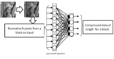
All the starting nodes of the GSOM are boundary nodes, i.e. each node has the freedom to grow in its own direction at the beginning. New Nodes are grown from the boundary nodes. Once a node is selected for growing all its free neighboring positions will be grown new nodes. In GSOM, input vectors are organized into categories depending on their similarity to each other. For data compression, the image or data is broken down into smaller vectors for use as input. For each input vector presented, the Euclidean distance to all the output nodes is computed. The weights of the node with the minimum distance, along with its neighboring nodes are adjusted. This ensures that the output of these nodes is slightly enhanced. This process is repeated until some criterion for termination is reached. After a sufficient number of input vectors have been presented, each output node becomes sensitive to a group of similar input vectors, and can therefore be used to represent characteristics of the input data. This means that for a very large number of input vectors passed into the network, (uncompressed image or data), the compressed form will be the data exiting from the output nodes of the network (considerably smaller number). This compressed data may then be further decompressed by another network. We take 50 neuron as a one input hidden layer and one output layer we take learning rate 0.5.the compression and decompression figure of GSOM Algorithm are following
Figure 1: GSOM Architecture compression
Pag e
24
Pag e24
Pag e24
Pag e24
Pag e24
Pag e24
Pag e24
Pag e24
Pag e24
Pag e24
Pag e24
Pag e24
Pag e24
Pag e24
Pag e24
Pag e24
Pag e24
Pag e24
Pag e24
Pag e24
Pag e24
4.2 The Learning Algorithm of the GSOM
The GSOM process is as follows:
1.Initialization phase
1. Initialize the weight vectors of the starting nodes (usually four) with random numbers between 0 and 1.
2. Calculate the growth threshold ( ) for the given data set of dimension according to the spread factor ( ) using the formula
2 . G r o w i ng Ph a s e
1. Present input to the network.
2. Determine the weight vector that is closest to the input vector mapped to the current feature map (winner), using
Euclidean distance. This step can be summarized as: find such that where , are the input and weight vectors respectively, is the position vector for nodes and is the set of natural numbers.
3. The weight vector adaptation is applied only to the neighborhood of the winner and the winner itself. The neighborhood is a set of neurons around the winner, but in the GSOM the starting neighborhood selected for weight adaptation is smaller compared to the SOM (localized weight adaptation). The amount of adaptation (learning rate) is also reduced exponentially over the iterations. Even within the neighborhood, weights that are closer to the winner are adapted more than those further away. The weight adaptation can be described by
where the Learning Rate , is a sequence of positive parameters converging to zero as . , are the weight vectors of the node before and after the adaptation and
is the neighborhood of the winning neuron at the th iteration. The decreasing value of in the GSOM depends on the number of nodes existing in the map at time .
4. Increase the error value of the winner (error value is the difference between the input vector and the weight vectors). 5. When (where is the total error of node and is the growth threshold). Grow nodes if i is a boundary
node. Distribute weights to neighbors if is a non-boundary node.
6. Initialize the new node weight vectors to match the neighboring node weights. 7. Initialize the learning rate ( ) to its starting value.
8. Repeat steps 2 – 7 until all inputs have been presented and node growth is reduced to a minimum level.
3. Smoothing phase.
Reduce learning rate and fix a small starting neighborhood. Find winner and adapt the weights of the winner and neighbors in the same way as in growing phase
4.2.1 Encoding
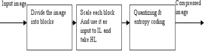
The trained network is now ready to be used for image compression which, is achieved by dividing or splitting the input images into blocks after that scaling and applying each block to the input of Input Layer (IL) then the output of Hidden layer HL is quantized and entropy coded to represent the compressed image. Entropy coding is lossless compression that will further squeeze the image; for instance, Huffman coding code be used here. Fig. (3) Show the encoding steps.
Figure 3: Encoding process of image compression
4.2.2 Decoding
25
25
25
25
25
25
25
25
25
25
25
25
25
25
25
25
25
25
25
25
25
Figure 4: Decoding process of image compression
5. Result Analysis
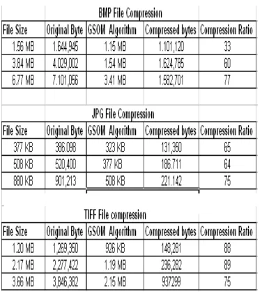
In order to test the compression engine, several files of various formats were run through the scheme. This system uses three metrics such as compression ratio, transmission time. Compression ratios are defined as [9].
Compression Ratio = 100 – Z
Table (1) show the compression ratio of various file such as BMP, JPG, TIFE
Table 1: Compression ratio of BMP, JPG, TIFE file
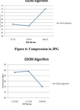
The graph for different compression ratio is
BMP File Size
Pag
e
26
Pag
e
26
Pag
e
26
Pag
e
26
Pag
e
26
Pag
e
26
Pag
e
26
Pag
e
26
Pag
e
26
Pag
e
26
Pag
e
26
Pag
e
26
Pag
e
26
Pag
e
26
Pag
e
26
Pag
e
26
Pag
e
26
Pag
e
26
Pag
e
26
Pag
e
26
Pag
e
26
Figure 6: Compression in JPG
Figure 7: Compression in TIFF
Identifying files as belonging to particular classes offers a quicker way of encoding and decoding the files. The GSOM Algorithm offers us a way of encoding knowledge as a set of training examples rather than by a set of rules and is an effective technique for problem domains where there are many rules or the rules cannot be easily devised. This research also shows that conventional computing and artificial neural networks are not in conflict with each other but each can be exploited for the advantages they offer
6. Future Enhancement
• Artificial Neural Networks is currently a hot research area in Data compression.
• GSOM algorithm for data compression being a wide field which is rapidly finding use in many applied fields and technologies
• GSOM has some limitation. They cannot compress higher size of audio and video file. So To Improve the Compression Ratio of higher size of audio and video file in future enhancement
7. Conclusion
Our main work is focused on the data compression by using Growing Self Organizing Map algorithm, which exhibits a clear-cut idea on application of multilayer perceptron with special features compare to Hoffman code. By using this algorithm we can save more memory space, and in case of web applications transferring of images and download should be fast. The propose approach (Gsom) are used to compressed the various image file such as BMP,JPG,TIFE etc and compression ratio is batter then other traditional algorithm such as Huffman ,LZW, Arithmetic etc.
27
27
27
27
27
27
27
27
27
27
27
27
27
27
27
27
27
27
27
27
27
8. References
[1]. R. C.Gonzales, R. E. Woods, Digital Image Processing, Second Edition, Prentice-Hall, 2002.
[2]. Veisi H., Jamzad M., Image Compression Using Neural Networks, Image Processing and Machine Vision Conference (MVIP), Tehran, Iran, 2005.
[3]. Missing Data Estimation Using Principle Component Analysis and Auto associative Neural Networks. Jaisheel Mistry, Fulufhelo V. Nelwamondo, Tshilidzi Marwala. 3, s.l. : iiisci.org, Journal of Systemics, Cybernatics and Informatics, Vol. 7, pp. 72-79, 2009,
[4]. B. Verma, M. Blumenstein, S. Kulkarni, "A new compression technique using an artificial neural network". Faculty of Information and Communication Technology, Griffith University, Australia, 2004.
[5]. M. Egmont-Petersen, D. de Ridder, H. Handles, "Image processing with neural networks- a review", Pattern Recognition , 35, pp. 2279- 2301, 2002.
[6]. J. Jiang, "Image compression with neural networks – A survey, Signal Processing": Image Communication, 14, pp. 737 – 760, 1999.
[7]. S. Anna Durai and E. Anna Saro “Image Compression with Back-Propagation Neural Network using Cumulative Distribution Function” World Academy of Science, Engineering and Technology 17, 2006.
[8]. Martin Riedmiller and Heinrich Braun “A Direct Adaptive Method for Faster Back propagation Learning: The RPROP Algorithm” Institute fur Logic, Komplexitat und Deduktionssyteme, University of Karlsruhe, W-7500 Karlsruhe, FRG, 1993.
[9]. Md. I. Bhuiyan, Md. K. Hassan, "Image compression with neural network using DC algorithm", Journal of signal processing, vol. 5, no. 6, pp. 445 -459, 2001
[10]. S.S Panda, M.S.R.S Prasad Ch.SKVR Naidu”Image compression using backpropagation neural network”, International journal of engineering science and advance technology volume -2,issue-1,2012 pp:74-78 ISSN:2250-3676.
[11]. Neelmani chhedaiya, prof. Vishal Moyal “Implementation of Backpropagation algorithm in Verilog”,International Journal Computer Technology and application volume-3,issue-1,2012, pp:340-343:ISSN:2229-6093.
[12]. K.Siva Nagi Reddy, Dr. B.R.Vikram, L. Koteswara Rao”Image Compression and reconstruction using a new approach by artificial neural network”, International journal of image processing “, volume -6, Issue-2, 2012, pp:68-85.
[13].Anuj Sharma & Mahendra Pratap Panigraphy” neural network and image compression”, VSRD-International journal of computer science and information technoology”,volume-2,Issue-9,2012,pp:746-755.
[14]. P.Nirupama 1 Senior Assistant Professor in CSE Dept, BVRIT 2 . Associate Professor in SE Dept ”Analysis of Various Image Compression Techniques” . vol,2no.4, May 2012. ARPN Journal of science and Technology
[15]. Mamta Sharma S.L. Bawa D.A.V. college Compression Using Huffman Coding IJCSNS International Journal of Computer Science and Network Security, VO .10 No.5, May 2010
Pag
e
28
Pag
e
28
Pag
e
28
Pag
e
28
Pag
e
28
Pag
e
28
Pag
e
28
Pag
e
28
Pag
e
28
Pag
e
28
Pag
e
28
Pag
e
28
Pag
e
28
Pag
e
28
Pag
e
28
Pag
e
28
Pag
e
28
Pag
e
28
Pag
e
28
Pag
e
28
Pag
e