An Optimization-Simulation
Approach to Chance-Constraint
Programming
ITC 2/47
Journal of Information Technology and Control
Vol. 47 / No. 2 / 2018 pp. 310-320
DOI 10.5755/j01.itc.47.2.18712 © Kaunas University of Technology
An Optimization-Simulation Approach to Chance-Constraint Programming
Received 2017/07/31 Accepted after revision 2018/05/11
http://dx.doi.org/10.5755/j01.itc.47.2.18712
Stefan Marković, MirkoVujošević, Dragana Makajić-Nikolić
Faculty of organisational sciences, University of Belgrade, Jove Ilića 154, Belgrade, SerbiaCorresponding author: [email protected]
This paper considers a stochastic programming problem with a number of random parameters in the set of constraints. The method used for solving the problem is the iterative optimization-simulation approach. It consists of two phases: optimization phase, which includes solving a deterministic counterpart of the original chance-constrained problem, and a simulation phase in which the original constraints are checked using Mon-te Carlo simulation. One iMon-teration corresponds to one scenario. If the decision maker is dissatisfied with the results, a new scenario is generated in which the deterministic values of stochastic parameters are changed in the direction that will provide a more robust solution. The deterministic counterpart in the new scenario is for-mulated depending on the result of the previous iteration. To that end, different heuristics are considered. The main goal is to provide a good insight on the optimization problem under uncertainty by performing a relatively small number of iterations. The general approach and results of the proposed framework are illustrated on an example of advertisement placement.
KEYWORDS: Stochastic programming, Simulation, Chance-constraints, Heuristics, Scenario generation.
1. Introduction
Chance-constrained programming (CCP) is a well-known approach to solving stochastic problems. It was first introduced in 1959 [8], where the optimization problem is formulated so that the probability of meet-ing a constraint is above a certain acceptable level. This changes the nature of the stochastic problem from one
Therefore, a novel optimization-simulation approach to solving CCP problem is proposed. Optimiza-tion-simulation approaches are not new to optimiza-tion, and their aim is to integrate optimization methods with Monte Carlo simulation experiments for solving stochastic problems [33, 18, 19, 45, 16, 7, 1, 32, 31]. Their number has increased significantly only recently, due to increased computational abilities of computers. Simulation is generally used as input for the other part of the framework ‒ optimization, to create determinis-tic models and solve them.
The novelty in the approach proposed in this paper is that the power of simulation is used to find the prob-ability of satisfying chance-constraints. Simulation is used to solve the hardest part of the CCP problem, by finding the probability of satisfying the constraints, which is often why CCP problems are intractable. The first phase of the approach ‒ the optimization phase, relies on generating appropriate deterministic counterparts of the original problem to be optimized. The efficient generation of such scenarios is the cen-tral problem in stochastic programming in general [9, 17, 41], so some simple heuristics are proposed. The proposed approach is illustrated using the problem of advertisement placement.
The paper is organized as follows: Section 2 formulates the advertisement placement model, i.e. the mathemat-ical model, notation, and a gives a short explanation of the optimization task; Section 3 is reserved for a de-tailed description of the proposed optimization-simu-lation approach; Section 4 shows the heuristics used to generate scenarios. Research results are presented in Section 5. Concise results are given in tables and dia-grams for every scenario used. Section 6 summarizes the conclusions.
2. Advertisement Placement
Problem
Operational research (OR) techniques were first ap-plied in marketing with the emergence of the famous theorem for marketing mix optimization in 1954 [15]. Linear programming and goal programming became first choices when talking about OR in marketing, and Markov models and various simulation
tech-niques, including game theory, were applied in the 1960’s and 1970’s [29,34]. Even in these early days of interaction between OR and marketing, researchers observed the stochastic nature of marketing prob-lems through utilizing the theory of decision mak-ing under uncertainty [38]. Not much was done in the upcoming years in the field. But recently, due to substantially increased computational capacities of computers, modeling uncertainty through various estimation techniques has found its place in OR ap-plications in marketing [39, 26, 3].
Consequently, stochastic programming is not new to marketing, but generally was not the main focus of researchers in the beginning. Nevertheless, it has sparked a new interest among researchers in various fields of marketing problems.
As part of the marketing mix, advertising was partic-ularly researched. However, researchers deemed its effects on sales and market share to be doubtful. This particular opinion was formed due to concerns that advertising might have no effect on sales. But, since [10, 30, 43, 14, 23] confirmed that advertising has a positive influence on sales, all suspicions on the ef-fectiveness of these models and its application in de-cision making were dismissed. Naturally, significant effort was put into developing models that could op-timize the allocation of an advertising budget, which is also the task of this paper.
The problem considered in this paper is the selection of the optimal number of advertisements to be placed in different newspapers. Apart from the obvious task of determining the number of advertisements, their positions and size for every newspaper have to be determined as well, while reaching the needed views and scores both in total population, and within target groups. The goal is to achieve all the aforementioned with the lowest cost possible. Daily, weekly and monthly newspapers, their total views and ratings for the targeted groups are considered. Ratings are data with a stochastic nature and are assumed to have a Gaussian distribution. The problem is formulated as a mixed-integer stochastic programming model. Notation
T - Set of target groups
S - Minimum number of unique advertisement views cij - Price for j-th position in i-th newspaper
vi - Number of i-th newspaper views
rik - i-th newspaper rating for k-th target group
pj - Visibility percentage for j-th advertisement position
tk - Wanted rating for k-th target group
mi- Minimum number of advertisement in i-th
news-paper
hi - Maximum number of advertisement in i-th
news-paper
gj - Minimum number of advertisement on j-th position
dj - Maximum number of advertisement on j-th position
xij- Number of j-th advertisement in i-th newspaper
Mathematical model
With reference to the introduced notation, the adver-tisement placement model follows:
Minimize
( )
i
ij ij i I j P
f x c x
∈ ∈
=
∑ ∑
(1)subject to constraints
, i
i j ij i I j P
v p x S ∈ ∈
≥
∑ ∑
(2)Pr , ,
i
ik ij k k i I j P
r x t p k T
∈ ∈
≥ ≥ ∈
∑ ∑
(3), ,
i
ij i j P
x m i I
∈
≥ ∈
∑
(4), ,
i
ij i j P
x h i I ∈
≤ ∈
∑
(5), ,
i
ij j i I j P
x g j J
∈ ∈
≥ ∈
∑
(6), .
i
ij j i I j P
x d j J
∈ ∈
≤ ∈
∑
(7)Constraint (2) ensures the minimum required ad-vertisement views; constraint (3) is a stochastic con-straint that sets the wanted rating for every target group; constraints (4) and (5) set the minimum and maximum number of possible advertisement for
ev-ery newspaper, respectively; and constraints (6) and (7) set the minimum and maximum total number of advertisement that can be placed on the assigned po-sitions in newspapers, respectively.
The stochastic nature of the model is reflected in equation (3), and in its set of constraints. The obvi-ous reason is the stochastic parameter rik, which
rep-resents the newspaper rating for target groups. These ratings are calculated based on the number of copies printed, newspaper reputation and tradition, and the position of advertisement placed in those newspa-pers. The method used to calculate these parameters is not the focus of this paper. For the purpose of the model, we considered a case where uncertain param-eters have a Gaussian distribution with expected val-ue - μ and variance - σ.
There are 14 different target groups, which gives us a set of 14 stochastic constraints to be considered. Target groups, and consequently the set of stochastic constraints, can be classified in four groups:
_ Gender: the first two constraints define the
minimum wanted rating achieved within male and female population,
_ Age: six different age categories are considered,
and consequently the same number of constraints that define minimum wanted ratings within every age group,
_ Geographic location: the model differentiates
between three geographic locations where newspapers are sold, hence the minimum ratings that need to be achieved within the assigned geographic region are set,
_ Education: three education levels are considered,
make further groups of constraints, but these are the general guidelines on how this specific problem was modeled in this paper.
3. Optimization-Simulation Approach
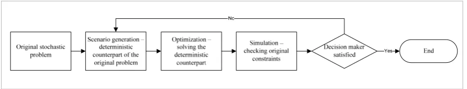
The approach consists of two phases ‒ the optimiza-tion phase, where scenarios are generated and the de-terministic model is solved to optimality using GLPK (GNU Linear Programming Kit - https://www.gnu. org/software/glpk/),and a simulation phase, where the validity of the scenario is tested by checking the chance-constraints through simulation.The main idea is to replace the original, stochastic problem with a new, deterministic model that will provide the best solution under the condition that constraints are satisfied with a predefined probabili-ty. Generating a new deterministic counterpart of the original model corresponds to one scenario. Obvious-ly, this approach will require defining a considerable number of scenarios that need to be checked in order to find a scenario that will achieve the wanted proba-bility of satisfying the constraints. The upside is that every iteration provides further understanding of the original problem.
The second phase of the method uses the power of simulation to check the generated scenario.
Upon solving the deterministic counterpart of the original problem in the first phase, an optimal solu-tion is obtained. This is needed to determine the prob-ability of satisfying the chance-constraints. Next, a random deterministic value for every stochastic pa-rameter is set. The values are determined from each stochastic parameter’s predefined set with assigned distribution. This way a matrix of random determin-istic values from stochastic parameters is generated,
or in other words, the randomness of stochastic data is simulated. Whether the constraints are satisfied or not is checked by taking into account the determinis-tic values of stochasdeterminis-tic parameters and optimal solu-tions of the scenario generated in the first phase. These simulations are repeated N times, generating N of these matrices, inserting the numbers into the constraints and then calculating if they are satis-fied or not. The probability for satisfying stochastic constraints can be calculated by counting how many times constraints were satisfied, using the following formula:
Number of cases when constraint was satisfied Total number of cases N
∗ 100
This is done for every constraint in model.
This approach is valid under the presumption that the decision maker is willing to accept a certain risk of constraints not being satisfied. In return, the value of the criterion function would be better than if the decision maker removed all uncertainty and accepted
a robust approach. If the decision maker is dissatisfied with the results, a new scenario is created, i.e. a new deterministic counterpart of the original problem, and the whole procedure is repeated. The new scenario is formulated depending on the results of the previous one, and the goal is to find a scenario that meets the minimum criteria set by the decision maker.
The whole approach is summarized in Figure 1.
Figure 1.Optimization-simulation approach
The main issue of the procedure is scenario generation, namely, how to define a new deterministic counterpart of the original problem. There is no strict rule in scenario generation, and it is strongly suggested to use different heuristics. The particular heuristics used will depend on the nature of the problem, the assumed distribution of the random data, and the experience of the decision maker. The heuristics used in this paper are explained in the following section.
4. Heuristics Used for Scenario
Generation
Effectiveness and efficiency of the optimization-simulation method relies heavily on heuristics. The reason for this is the infinite number of possible scenarios to be considered. Heuristics are the cornerstone of the whole method.
Heuristic strategies are simple rules of thumb that solve complex uncertain situations [12]; they are “efficient cognitive processes that ignore information” [20] and “cognitive shortcuts that emerge when information, time and processing capacity are limited” [36].
Heuristics play a key role when facing complex problems under conditions of high uncertainty [35,24]. Simple-rules strategy of few heuristics are desirable in predictable environments, but are indispensable in unpredictable environments [13, 21, 4, 6, 11].
Nevertheless, heuristics are not shortcuts to solving complex problems at the expense of reduced processing time, but rely heavily on environmental
information [2, 25, 37]. By acknowledging these facts, heuristics can be ecologically rational. Ecological rationality is determined by two key factors, structure of the environment and lack of computing speed and power to solve the problem exactly due to a bounded rationality [42].
Ecological rationality lies in the foundation of the fast-and-frugal paradigm that provides a positive view on the heuristics, which is also the standpoint in this paper.
Fast and frugal heuristics will enable finding the right scenario by generating a relatively small number of scenarios, which is key to efficiency and effectiveness of the whole method. Considering the observed problem of advertisement placement, the distribution of the stochastic parameters and the desired pk levels, we present heuristics used to
efficiently search through the scenarios.
4.1. Heuristic 1
The first two scenarios to be generated correspond to deterministic doubles whose stochastic parameters are set to μ and μ-3σ respectively.
The μ-3σ scenario represents the robust scenario and, consequently, pk levels expected for this scenario are
1. Constraints are satisfied regardless of the realizations of the stochastic parameters. The reason this scenario is first checked is that the decision maker expects high pk levels (above 0.9 and 0.95) for
the acceptable scenario, which means that the wanted scenario is expected to be somewhere near the robust one.
The scenario with expected values μ gives the first insight into the nature of the observed problem. After checking the scenario using simulation, pk levels are This is done for every constraint in model.
This approach is valid under the presumption that the decision maker is willing to accept a certain risk of constraints not being satisfied. In return, the value of the criterion function would be better than if the decision maker removed all uncertainty and accept-ed a robust approach. If the decision maker is dis-satisfied with the results, a new scenario is created, i.e. a new deterministic counterpart of the original problem, and the whole procedure is repeated. The new scenario is formulated depending on the results of the previous one, and the goal is to find a scenario that meets the minimum criteria set by the decision maker.
The whole approach is summarized in Figure 1. The main issue of the procedure is scenario genera-tion, namely, how to define a new deterministic coun-terpart of the original problem. There is no strict rule in scenario generation, and it is strongly suggested to use different heuristics. The particular heuristics
Figure 1
Optimization-simulation approach
Number of cases when constraint was satisfied Total number of cases N
∗ 100
This is done for every constraint in model.
This approach is valid under the presumption that the decision maker is willing to accept a certain risk of constraints not being satisfied. In return, the value of the criterion function would be better than if the decision maker removed all uncertainty and accepted
a robust approach. If the decision maker is dissatisfied with the results, a new scenario is created, i.e. a new deterministic counterpart of the original problem, and the whole procedure is repeated. The new scenario is formulated depending on the results of the previous one, and the goal is to find a scenario that meets the minimum criteria set by the decision maker.
The whole approach is summarized in Figure 1.
Figure 1.Optimization-simulation approach
The main issue of the procedure is scenario generation, namely, how to define a new deterministic counterpart of the original problem. There is no strict rule in scenario generation, and it is strongly suggested to use different heuristics. The particular heuristics used will depend on the nature of the problem, the assumed distribution of the random data, and the experience of the decision maker. The heuristics used in this paper are explained in the following section.
4. Heuristics Used for Scenario
Generation
Effectiveness and efficiency of the optimization-simulation method relies heavily on heuristics. The reason for this is the infinite number of possible scenarios to be considered. Heuristics are the cornerstone of the whole method.
Heuristic strategies are simple rules of thumb that solve complex uncertain situations [12]; they are “efficient cognitive processes that ignore information” [20] and “cognitive shortcuts that emerge when information, time and processing capacity are limited” [36].
Heuristics play a key role when facing complex problems under conditions of high uncertainty [35,24]. Simple-rules strategy of few heuristics are desirable in predictable environments, but are indispensable in unpredictable environments [13, 21, 4, 6, 11].
Nevertheless, heuristics are not shortcuts to solving complex problems at the expense of reduced processing time, but rely heavily on environmental
information [2, 25, 37]. By acknowledging these facts, heuristics can be ecologically rational. Ecological rationality is determined by two key factors, structure of the environment and lack of computing speed and power to solve the problem exactly due to a bounded rationality [42].
Ecological rationality lies in the foundation of the fast-and-frugal paradigm that provides a positive view on the heuristics, which is also the standpoint in this paper.
Fast and frugal heuristics will enable finding the right scenario by generating a relatively small number of scenarios, which is key to efficiency and effectiveness of the whole method. Considering the observed problem of advertisement placement, the distribution of the stochastic parameters and the desired pk levels, we present heuristics used to efficiently search through the scenarios.
4.1. Heuristic 1
The first two scenarios to be generated correspond to deterministic doubles whose stochastic parameters are set to μ and μ-3σ respectively.
The μ-3σ scenario represents the robust scenario and, consequently, pk levels expected for this scenario are 1. Constraints are satisfied regardless of the realizations of the stochastic parameters. The reason this scenario is first checked is that the decision maker expects high pk levels (above 0.9 and 0.95) for the acceptable scenario, which means that the wanted scenario is expected to be somewhere near the robust one.
used will depend on the nature of the problem, the as-sumed distribution of the random data, and the expe-rience of the decision maker. The heuristics used in this paper are explained in the following section.
4. Heuristics Used for Scenario
Generation
Effectiveness and efficiency of the optimization-sim-ulation method relies heavily on heuristics. The rea-son for this is the infinite number of possible scenari-os to be considered. Heuristics are the cornerstone of the whole method.
Heuristic strategies are simple rules of thumb that solve complex uncertain situations [12]; they are “ef-ficient cognitive processes that ignore information” [20] and “cognitive shortcuts that emerge when in-formation, time and processing capacity are limited” [36].
Heuristics play a key role when facing complex prob-lems under conditions of high uncertainty [35, 24]. Simple-rules strategy of few heuristics are desirable in predictable environments, but are indispensable in unpredictable environments [13, 21, 4, 6, 11].
Nevertheless, heuristics are not shortcuts to solving complex problems at the expense of reduced pro-cessing time, but rely heavily on environmental in-formation [2, 25, 37]. By acknowledging these facts, heuristics can be ecologically rational. Ecological ra-tionality is determined by two key factors, structure of the environment and lack of computing speed and power to solve the problem exactly due to a bounded rationality [42].
Ecological rationality lies in the foundation of the fast-and-frugal paradigm that provides a positive view on the heuristics, which is also the standpoint in this paper.
Fast and frugal heuristics will enable finding the right scenario by generating a relatively small number of scenarios, which is key to efficiency and effective-ness of the whole method. Considering the observed problem of advertisement placement, the distribu-tion of the stochastic parameters and the desired pk levels, we present heuristics used to efficiently search through the scenarios.
4.1. Heuristic 1
The first two scenarios to be generated correspond to deterministic doubles whose stochastic parameters are set to μ and μ-3σ respectively.
The μ-3σ scenario represents the robust scenario and, consequently, pk levels expected for this scenario are
1. Constraints are satisfied regardless of the realiza-tions of the stochastic parameters. The reason this scenario is first checked is that the decision maker ex-pects high pk levels (above 0.9 and 0.95) for the
accept-able scenario, which means that the wanted scenario is expected to be somewhere near the robust one. The scenario with expected values μ gives the first in-sight into the nature of the observed problem. After checking the scenario using simulation, pk levels are
calculated for all of the 14 chance-constraints. It is to be expected that all active constraints will have pk
lev-els at around0.5, while inactive ones will be at around 0.9 or above. There will be a third group of constraints between active and inactive ones.
This heuristic indicates the existing constraints: ac-tive - stochastic parameters in these constraints need to be moved in the subsequent scenarios towards the robust solution to get the desired pi; inactive - con-straints which already meet the set pi and whose stochastic parameters should not be changed; con-straints between the previous two - whose stochastic parameters need to be moved to some extent towards the robust solution, depending on the results of the simulation for the scenarios.
4.2. Heuristic 2
Exploit the positive correlation between the constraints within the groups when generating new scenarios. Positive correlation between the constraints with-in groups is hypothesized, but to a different extent among groups. Therefore, three heuristics are derived from this general one:
Heuristic 2.1:
There is a strong positive correlation within the con-straints in the age group.
little to no positive correlation between age groups 12-19 and 66+. The positive correlation between con-straints within an age group increases or decreases correspondingly.
Heuristic 2.2:
There is no positive or negative correlation within the gender group of constraints.
Since the male and female population have differ-ent interests in newspapers and magazines, there is no significant correlation to be expected to be of use when generating scenarios.
Heuristic 2.3:
For the remaining two groups of constraints, geograph-ic region and education, there is a moderate positive correlation to be expected and taken into account when generating new scenarios.
The most important knowledge obtained through this second group of heuristics is that it gives further in-sight into the problem and indicates the relations that exist between the stochastic constraints.
This means that it will not be necessary to create scenarios that will be closer to a robust one for all the parameters in every constraint in consecutive it-erations, but only for some constraints. In exchange, one can still expect an increase in pk levels for all
constraints within groups. By applying this heuris-tic, both of the prerequisites for a good scenario are achieved: high probability levels for constraint satis-faction, and a better value of criterion function.
4.3. Heuristic 3
Determine the “simulation step”.
The simulation step is defined as the value for which the stochastic parameters are adjusted when gener-ating a new deterministic equivalent of the original problem. In this paper, the simulation step is fixed to 0.1σ, meaning that when generating a new scenario, deterministic values of the stochastic parameters are adjusted by 0.1σ towards the robust parameters, rela-tive to the previous scenario.
The first heuristic indicated the constraints whose parameters need to be changed and to what extent; the second heuristic provided an insight into the re-lations of constraints within groups, further reducing the need to linearly change all of the parameters in
the designated constraints; and the final heuristic de-termined the concrete value for which the stochastic parameters are adjusted.
It provides consistency when generating new scenar-ios and enables the decision maker to get an insight into the sensitivity of the constraints when changing stochastic parameters through consecutive scenari-os.
Simulation step can be defined as declining, meaning that it decreases as scenarios get closer to a robust scenario, or it can be mixed, which is the combination of the fixed and declining step. Since heuristics are idiosyncratic by its very nature, [4], decision makers can use simulation steps best suited for their problem. This concludes the list of heuristics used and is fol-lowed by the results.
5. Computational Testing and Results
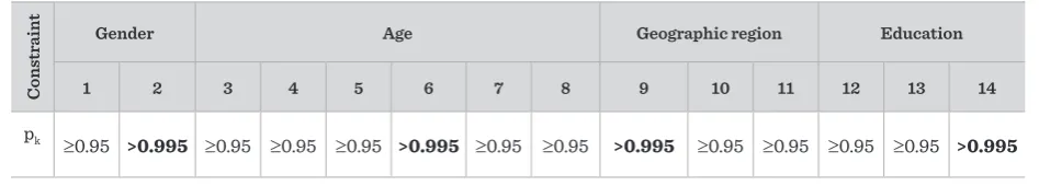
The set of 14 stochastic constraints, defined by equa-tion (3) in the model formulaequa-tion, are chance-con-straints with a predefined probability level of satis-faction pk.The decision maker sets the pk level for every
con-straint. The decision maker owns a chain of super-markets and therefore wants to target a specific group through advertising. His target group are women aged between 40 and 49, from the geographical region G1, with a university degree. This means that second, sixth, ninth and fourteenth constraint need to have the highest pk level. The decision maker is willing to
accept less than 0.005 risk that these constraints will not be satisfied, which means that pk levels for these
four constraints need to be higher than 0.995. For all other constraints, the decision maker is willing to ac-cept a 0.05 risk, namely, pk levels are equal or higher
than 0.95. This is presented in Table 1.
In return, the decision maker demands at least 15% in currency less spent than if the robust approach was to be used on this model. So the tradeoff is described by accepting certain levels of risk in return for a better value of criterion function.
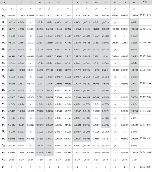
The columns denote14 target groups, TGk, k=1,…,14
as presented in the model formulation in Section 3. The last column represents the value of the criterion function. Changes in its value can be tracked through different scenarios. Rows of the table represent the scenario, with allocated deterministic values of the stochastic parameters, and for each scenario there is a pk level indication that shows the probability of
sat-isfying the constraints.
Scenario with expected value (Sexp) and robust
sce-nario (Srob) are two marginal cases designated by the
heuristic 1, and scenarios are generated between these two cases. For each scenario there is an indi-cation what the new deterministic equivalent is set to, and the following row presents the probability of satisfying chance-constraints of the scenario. Each scenario is run through 10,000 simulations and ap-propriate probabilities are calculated and presented in the table. Shaded cells indicate that changes were made to the scenario for the assigned constraint, rel-ative to the previous scenario. The desired scenario is S10 as it meets the wanted pk levels and the value of
criterion function set by the decision maker.
The value of the criterion function is the worst for the robust scenario Srob, which is expected, since it
removes all uncertainty from the model. The lowest and the best value of the criterion function is for the scenario with the expected values, but chances that constraints are satisfied are the lowest. The value of the criterion function increases slowly as we move towards the desired scenario S10 that gives us the
de-sirable probabilities for chance-constraints, keeping them within the risk accepted by the decision maker. By comparing the values of the criterion functions between the robust scenario and the desirable S10,
there is an 18,4% decrease in the value of the function, which meets the limit set by the decision maker.
We draw your attention to the fact that only ten sce-narios are presented in the results section due to the limited space of the paper, and with the aim of a clear-er presentation of results.
Note that the number of possible scenarios (itera-tions) in the observed stochastic problem is infinite. Even a simple discretization of the probability dis-tributions for stochastic parameters leads to an ex-ponential growth of the number of iterations and scenarios to be checked. The main goal of the optimi-zation-simulation approach is to reduce the number of scenarios to a reasonable level.
We would like to refer our readers to the following book [40], especially Chapter 6, which considers the issue of generating and checking scenarios of sto-chastic programming problems with Monte-Carlo simulation to full extent.
As for our problem, scenarios are generated and checked until minimal requirements of the decision maker are met. In our case, it meant generating exact-ly 112 different scenarios before reaching the desired probabilities for constraints and the wanted value of the criterion function. Having in mind that the CPU time for the optimization part is 10.5 seconds and for the simulation part 2 seconds (RAM: 4.00GB; Proces-sor: Intel (R) Core (TM) i3-2310M 2.10GHz), reach-ing the desired scenario for such a complex problem was not time consuming.
For the sake of clarity, only ten key scenarios are pre-sented. The results presented show the general ap-proach, how the heuristics were checked, and new heuristic rules acquired and applied when solving this problem.
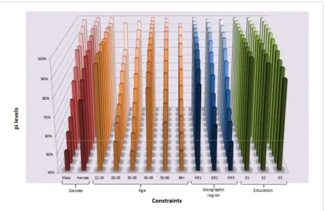
Figure 2 graphically summarizes the results of the computational testing of scenarios:
Each group of constraints has its own color, and a to-Table 1
Probability levels for soft constraints
Cons
tr
ain
t
Gender Age Geographic region Education
1 2 3 4 5 6 7 8 9 10 11 12 13 14
pk Srob pk S10 pk S9 pk S8 pk S7 pk S6 pk S5 pk S4 pk S3 pk S2 pk S1 pk Sexp TGk 1 μ-3σ 0.9864 μ-0.9σ 0.9658 μ-0.9σ 0.9432 μ-0.8σ 0.8896 μ-0.7σ 0.8923 μ-0.6σ 0.8151 μ-0.5σ 0.7640 μ-0.4σ 0.6881 μ-0.3σ 0.6184 μ-0.2σ 0.5715 μ-0.1σ 0.5061 μ 1 1 μ-3σ 0.9981 μ-0.9σ 0.995 μ-0.9σ 0.99 μ-0.8σ 0.9933 μ-0.7σ 0.9724 μ-0.6σ 0.9618 μ-0.5σ 0.9336 μ-0.4σ 0.9273 μ-0.3σ 0.8864 μ-0.2σ 0.8531 μ-0.1σ 0.7769 μ 2 1 μ-3σ 0.9994 μ 0.9838 μ 0.9822 μ 0.9961 μ 0.9921 μ 0.9774 μ 0.9818 μ 0.9921 μ 0.973 μ 0.9883 μ 0.9648 μ 3 1 μ-3σ 0.9666 μ-1.5σ 0.8214 μ-0.9σ 0.8048 μ-0.8σ 0.7848 μ-0.7σ 0.7661 μ-0.6σ 0.72 μ-0.5σ 0.6859 μ-0.4σ 0.6595 μ-0.3σ 0.6231 μ-0.2σ 0.6222 μ-0.1σ 0.5549 μ 4 1 μ-3σ 0.9772 μ-1σ 0.9431 μ-0.9σ 0.9079 μ-0.8σ 0.8795 μ-0.7σ 0.8455 μ-0.6σ 0.7776 μ-0.5σ 0.7208 μ-0.4σ 0.6687 μ-0.3σ 0.6189 μ-0.2σ 0.5646 μ-0.1σ 0.5021 μ 5 1 μ-3σ 0.999 μ-0.5σ 0.9988 μ-0.5σ 0.9985 μ-0.5σ 0.9969 μ-0.5σ 0.9903 μ-0.5σ 0.9808 μ-0.5σ 0.9684 μ-0.4σ 0.9602 μ-0.3σ 0.9231 μ-0.2σ 0.8944 μ-0.1σ 0.8416 μ 6 1 μ-3σ 0.9942 μ-0.5σ 0.9902 μ-0.5σ 0.9816 μ-0.5σ 0.9783 μ-0.5σ 0.9514 μ-0.5σ 0.9185 μ-0.5σ 0.8775 μ-0.4σ 0.837 μ-0.3σ 0.7733 μ-0.2σ 0.7297 μ-0.1σ 0.658 μ 7 1 μ-3σ 0.9621 μ-0.9σ 0.9627 μ-0.9σ 0.9323 μ-0.8σ 0.9057 μ-0.7σ 0.8539 μ-0.6σ 0.8038 μ-0.5σ 0.7379 μ-0.4σ 0.6876 μ-0.3σ 0.6255 μ-0.2σ 0.5659 μ-0.1σ 0.506 μ 8 1 μ-3σ 0.9995 μ-0.9σ 0.9985 μ-0.9σ 0.9963 μ-0.8σ 0.9962 μ-0.7σ 0.9917 μ-0.6σ 0.9847 μ-0.5σ 0.9727 μ-0.4σ 0.9609 μ-0.3σ 0.9358 μ-0.2σ 0.9084 μ-0.1σ 0.8594 μ 9 1 μ-3σ 0.9909 μ-0.6σ 0.9898 μ-0.6σ 0.9787 μ-0.6σ 0.9722 μ-0.6σ 0.944 μ-0.6σ 0.902 μ-0.5σ 0.8610 μ-0.4σ 0.8251 μ-0.3σ 0.7492 μ-0.2σ 0.706 μ-0.1σ 0.6457 μ 10 1 μ-3σ 0.9881 μ-0.8σ 0.9722 μ-0.8σ 0.9502 μ-0.8σ 0.9379 μ-0.7σ 0.8981 μ-0.6σ 0.8503 μ-0.5σ 0.7843 μ-0.4σ 0.74 μ-0.3σ 0.6662 μ-0.2σ 0.6291 μ-0.1σ 0.5541 μ 11 1 μ-3σ 1 μ 1 μ 1 μ 1 μ 1 μ 1 μ 0.9999 μ 0.9998 μ 0.9994 μ 0.9993 μ 0.997 μ 12 1 μ-3σ 0.9999 μ 0.9991 μ 0.9984 μ 0.9992 μ 0.9986 μ 0.9953 μ 0.9934 μ 0.9952 μ 0.983 μ 0.9858 μ 0.9673 μ 13 1 μ-3σ 0.9985 μ-0.7σ 0.9969 μ-0.7σ 0.9939 μ-0.7σ 0.9936 μ-0.7σ 0.9892 μ-0.6σ 0.9777 μ-0.5σ 0.9662 μ-0.4σ 0.9583 μ-0.3σ 0.9315 μ-0.2σ 0.9208 μ-0.1σ 0.8899 μ 14 29.737.023 24.261.686 23.986.632 23.774.668 23.575.284 23.397.780 23.202.696 23.001.124 22.822.944 22.666.504 22.507.346 22.355.928 f (x) Table 2
Computational results – target groups and scenarios
tal of 11 scenarios are presented here, all but the ro-bust one. This chart shows how pk levels increase with
every new scenario.
The optimization simulation approach proposed in this paper is absolutely dependent on heuristics. Heuristics are what drive this method from the be-ginning until the end. On the other hand, the approach provides a perfect platform for the validation of the proposed heuristics. Hogarth and Karelaia show that simulation with computer-generated data is an ex-cellent way to evaluate a heuristic [25], meaning that whilst checking the generated scenarios, heuristics are being validated simultaneously. Heuristics also capitalize on learning processes [44]. This way the decision maker gets an insight into the problem and learns about the nature of the problem itself. This win-win situation provides a perpetual checking and learning process for both ends of the method ‒ sce-nario checking and heuristic validation.
Figure 2
Graphical representation of computational resultsFigure 2 graphically summarizes the results of the computational testing of scenarios: Figure 2Graphical representation of computational results
Each group of constraints has its own color, and a total of 11 scenarios are presented here, all but the robust one. This chart shows how pk levels increase
with every new scenario.
The optimization simulation approach proposed in this paper is absolutely dependent on heuristics. Heuristics are what drive this method from the beginning until the end. On the other hand, the approach provides a perfect platform for the validation of the proposed heuristics. Hogarth and Karelaia show that simulation with computer-generated data is an excellent way to evaluate a heuristic [25], meaning that whilst checking the generated scenarios, heuristics are being validated simultaneously. Heuristics also capitalize on learning processes [44]. This way the decision maker gets an insight into the problem and learns about the nature of the problem itself. This win-win situation provides a perpetual checking and learning process for both ends of the method ‒ scenario checking and heuristic validation.
Short computation time and memory, limited number of simulations considered and the speed with which the method is run makes it ideal for generating and testing new heuristics on similar problems.
6. Conclusion
In this paper, an original approach for tackling uncertainty in chance-constraint programming was put forward and general guidelines on how to use an optimization-simulation approach were given. Advertisement placement model, which is by nature a stochastic problem, was used to show how the optimization-simulation model could be applied in practice. The approach relies on heuristics when generating new scenarios. Heuristics are obtained through scenario testing, and the goal of the paper was to confirm them so they could be used in solving similar problems.
Computational testing shows that the approach is valid under the assumptions given in this paper. It also shows that we can obtain valid approximate solution to chance-constraint programming problem of advertisement placement by following the guidelines of the method. Knowledge obtained in solving this particular problem can be used as a basis for solving similar problems.
Short computation time and memory, limited number of simulations considered and the speed with which the method is run makes it ideal for generating and testing new heuristics on similar problems.
6. Conclusion
Computational testing shows that the approach is valid under the assumptions given in this paper. It also shows that we can obtain valid approximate solu-tion to chance-constraint programming problem of
advertisement placement by following the guidelines of the method. Knowledge obtained in solving this particular problem can be used as a basis for solving similar problems.
References
1. Arnold, U., Yildiz, Ö. Economic Risk Analysis of Decen-tralized Renewable Energy Infrastructures – A Monte Carlo Simulation Approach. Renewable Energy, 2015, 77, 227–239. doi:10.1016/j.renene.2014.11.059
2. Asta S., Özcan E., Parkes, A. J. CHAMP: Creating heu-ristics Via Many Parameters for online Bin Packing. Expert Systems with Applications, 2016, 63, 208–221. https://doi.org/10.1016/j.eswa.2016.07.005
3. Beltran-Royo, C., Escudero, L. F., Zhang, H. Multipe-riod Multiproduct Advertising Budgeting: Stochastic Optimization Modeling. Omega, 2016, 59, 26–39. doi. org/10.1016/j.omega.2015.02.013
4. Bingham, C. B., Eisenhardt, K. M. Rational Heuristics: The “Simple Rules” That Strategists Learn From Pro-cess Experience. Strategic Management Journal, 2011, 32, 1437–1464. doi:10.1002/smj.965
5. Birge, J., Louveaux, F. Introduction to Stochastic Pro-gramming. Springer, Berlin, 1997.
6. Bruni, M. E., Beraldi, P., Conforti, D. A Stochastic Pro-gramming Approach for Operating Theatre Schedul-ing Under Uncertainty. IMA Journal of Management Mathematics, 2015, 26, 99–119. https://doi.org/10.1093/ imaman/dpt027
7. Buyukada, M. Co-Combustion of Peanut Hull and Coal Blends: Artificial Neural Networks Modeling, Parti-cle Swarm Optimization and Monte Carlo Simula-tion. Bioresource Technology, 2016, 216, 280–286. doi. org/10.1016/j.biortech.2016.05.091
8. Charnes, A., Cooper, W. W. Chance-Constrained Pro-gramming. Management Science, 1959, 6, 73–79. https://doi.org/10.1287/mnsc.6.1.73
9. Chen M, Mehrotra S, Papp D. Scenario Generation for Stochastic Optimization Problems Via The Sparse Grid Method. Computational Optimization and Ap-plications, 2015, 62, 669–692. https://doi.org/10.1007/ s10589-015-9751-7
10. Clarke, D. G. Econometric Measurement of the Dura-tion of Advertising Effect on Sales. Journal of Market-ing Research, 1976, 13, 345–357. doi:10.2307/3151017
11. Crainic, T. G, Gobbato, L., Perboli, G., Rei, W. Logistics Capacity Planning: A Stochastic Bin Packing Formula-tion and a Progressive Hedging Meta-Heuristic. Euro-pean Journal of Operational Research, 2016, 253, 404– 417. https://doi.org/10.1016/j.ejor.2016.02.040
12. Czerlinski, J., Gigerenzer, G., Goldstein, D. G. How Good Are Simple Heuristics? Simple Heuristics That Make Us Smart, Oxford University Press, New York, 1999. 13. Davis, J. P., Eisenhardt, K. M., Bingham, C. B. Optimal
Structure, Market Dynamism, and the Strategy of Sim-ple Rules. Administrative Science Quarterly, 2009, 54, 413–452. https://doi.org/10.2189/asqu.2009.54.3.413 14. de Vries, L., Gensler, S., Leeflang, P. S. H. Effects of
Traditional Advertising and Social Messages on Brand-Building Metrics and Customer Acquisition. Journal of Marketing, 2017, 81, 1–15. doi.org/10.1509/ jm.15.0178
15. Dorfman, R., Steiner, P. O. Optimal Advertising and Op-timal Quality. The American Economic Review, 1954, 44, 826–836.
16. Dufo-Lopez, R., Pérez-Cebollada, E., Bernal-Agustín, J. L., Martinez-Ruiz, I. Optimisation of Energy Supply at Off-Grid Healthcare Facilities Using Monte Carlo Sim-ulation. Energy Conversion and Management, 2016, 113, 321–330. doi.org/10.1016/j.enconman.2016.01.057 17. Dupačová, J., Growe-Kuska, N., Romisch, W.
Scenar-io ReductScenar-ion in Stochastic Programming. Mathe-matical Programming, 2003, 95, 493–511. https://doi. org/10.1007/s10107-002-0331-0
18. Fu, M. C, Price, C. C, Zhu, J., Hillier, F. S. Handbook of Simulation Optimization. Springer-Verlag, New York, 2015.
19. Ge, H., Nolan, J., Gray, R., Goetz, S., Han, Y. Supply Chain Complexity and Risk Mitigation – A Hybrid Op-timization–Simulation Model. International Journal of Production Economics, 2016, 179, 228–238. https://doi. org/10.1016/j.ijpe.2016.06.014
Cog-nitive Science, 2009, 1, 107–143. doi:10.1111/j.1756-8765.2008.01006.x
21. Goldstein, D. G., Gigerenzer, G. Models of Ecological Ra-tionality: The Recognition Heuristic. Psychological Re-view, 2002, 109, 75–90. http://dx.doi.org/10.1037/0033-295X.109.1.75
22. Hanasusanto, G. A., Kuhn, D., Wiesemann, W. A Comment on “Computational Complexity of Stochastic Program-ming Problems.” Mathematical ProgramProgram-ming, 2016, 159, 557–569. https://doi.org/10.1007/s10107-015-0958-2 23. Hartnett, N., Kennedy, R., Sharp, B., Greenacre, L.
Cre-ative that Sells: How Advertising Execution Affects Sales. Journal of Advertising, 2016, 45, 102–112. https:// doi.org/10.1080/00913367.2015.1077491
24. Helfat, C., Peteraf, M. Managerial Cognitive Capabili-ties and the Microfoundations of Dynamic CapabiliCapabili-ties. Strategic Management Journal, 2014, 36, 831-850. doi: 10.1002/smj.2247
25. Hogarth, R. M., Karelaia, N. Heuristic and Linear Mod-els of Judgment: Matching Rules and Environments. Psychological Review, 2007, 114, 733–758. http://dx.doi. org/10.1037/0033-295X.114.3.733
26. Illner, R., Ma, J. An SIS-type Marketing Model on Ran-dom Networks. Communications in Mathematical Sci-ences, 2016, 14, 1723–1740. http://dx.doi.org/10.4310/ CMS.2016.v14.n6.a12
27. Kall, P., Mayer, J. Stochastic Linear Programming. Springer, Berlin, 2005.
28. Kendall, J. W. Hard and Soft Constraints in Linear Programming. Omega, 1975,3, 709–715. https://doi. org/10.1016/0305-0483(75)90073-0
29. Kotler P. The Use of Mathematical Models in Mar-keting. Journal of Marketing, 1963, 27, 31–41. doi:10.2307/1248643
30. Leone, R. P., Schultz, R. L. A Study of Marketing Gen-eralizations. Journal of Marketing, 1980, 44, 10–28. doi:10.2307/1250029
31. Mavrotas, G., Pechak, O., Siskos, E., Doukas, H., Psar-ras, J. Robustness Analysis in Multi-Objective Mathe-matical Programming Using Monte Carlo Simulation. European Journal of Operational Research, 2015, 240, 193–201. https://doi.org/10.1016/j.ejor.2014.06.039 32. Meeds, E., Welling, M. Optimization Monte Carlo:
Effi-cient and Embarrassingly Parallel Likelihood-Free
In-ference. Neural Information Processing Systems Con-ference, 2015, 1–9.
33. Mokhtari, H., Salmasnia, A. A Monte Carlo Simulation Based Chaotic Differential Evolution Algorithm for Scheduling a Stochastic Parallel Processor System. Ex-pert Systems with Applications, 2015, 42, 7132–7147. dx.doi.org/10.1016/j.eswa.2015.05.015.
34. Montgomery, D. B. Applications of Management Sci-ence in Marketing. Prentice-Hall, Englewood Cliffs (N.J.), 1970.
35. Mousavi, S., Gigerenzer, G. Risk, Uncertainty, and Heu-ristics. Journal of Business Research, 2014, 67, 1671– 1678. doi:10.1016/j.jbusres.2014.02.013
36. Newell, A., Simon, H. A. Human Problem Solving. Pren-tice Hall, Englewood Cliffs (N.J.), 1971.
37. Payne, J. W., Bettman, J. R., Johnson, E. J. The Adaptive Decision Maker, Cambridge University Press, Cam-bridge, 1993.
38. Pratt, J., Raiffa, H., Schlaifer, R. Introduction to Statisti-cal Decision Theory, 1995.
39. Rossi, P. E., Allenby, G. M. Bayesian Statistics and Mar-keting. Marketing Science, 2003, 22, 304–328. https:// doi.org/10.1287/mksc.22.3.304.17739
40. Ruszczyński, A., Shapiro, A. Stochastic Programming, Handbooks in Operations Research and Management Science. Elsevier, Amsterdam, 2003.
41. Shapiro, A., Dentcheva, D., Ruszczyński, A. Lectures on Stochastic Programming. MOS-SISAM Series on Opti-mization, Philadelphia, 2009.
42. Simon, H. A. Invariants of Human Behavior. Annu-al Review of Psychology, 1990, 41, 1–19. https://doi. org/10.1146/annurev.ps.41.020190.000245
43. Vidale, M. L., Wolfe, H. B. An Operations-Research Study of Sales Response to Advertising. Operations Research, 1957, 5, 370–381. https://doi.org/10.1287/opre.5.3.370 44. Wübben, M., Wangenheim F. V. Instant Customer Base
Analysis: Managerial Heuristics Often “Get It Right.” Journal of Marketing, 2008, 72, 82–93. http://www. jstor.org/stable/30162213