Magnetic airborne survey – geophysical flight
Erick de Barros Camara1and Suze Nei Pereira Guimarães2 1Brucelandair, Ontario, Canada
2Prospectors Aerolevantamentos e Sistemas Ltda, Rio de Janeiro, Brazil
Correspondence to:Erick de Barros Camara (erickcamara@msn.com)
Received: 16 December 2015 – Published in Geosci. Instrum. Method. Data Syst. Discuss.: 2 February 2016 Revised: 9 May 2016 – Accepted: 19 May 2016 – Published: 6 June 2016
Abstract.This paper provides a technical review process in the area of airborne acquisition of geophysical data, with em-phasis for magnetometry. In summary, it addresses the cali-bration processes of geophysical equipment as well as the aircraft to minimize possible errors in measurements. The corrections used in data processing and filtering are demon-strated with the same results as well as the evolution of these techniques in Brazil and worldwide.
1 Introduction
Geophysics is the branch of science that involves the study of the Earth’s physical measurements. There are many types of geophysical measurements that can be made. Airborne geo-physics deals with one of them. It uses data acquired in air-borne surveys in assessment of mineral exploration potential over large areas. Measurements are usually made at an early stage of the exploration process, which can be of consider-able help also in classification of soil types in the area.
The first geophysical airborne research method was the magnetic method. Discovered by Faraday, Sect. XIX, the method was initially employed by the USSR (currently Rus-sia) in 1936 (Hood and Ward, 1969) and adapted later with better modifications by the United States in 1940 (Hood and Ward, 1969). Both countries had vested interests in military and technology, particularly for submarine applica-tions. After some improvements, another early airborne sur-vey was made in the US in 1944 using the Beech Stagger-wing NC18575 (Morrison, 2004).
The first geophysical airborne survey in Brazil was carried out 60 years ago (1953) in the city of Sao Joao Del Rey, state of Minas Gerais (Hildebrand, 2004). It was conducted by the Prospec Company, which later became Geomag. The survey
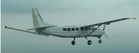
utilized both magnetic and radiometric methods. The fixed-wing aircraft PBY-5 (Catalina) was used in the survey. It was equipped with a Fluxgate magnetometer in the tail of the air-craft, which measured the total magnetic field (Hildebrand, 2004). The system was entirely analogue type, constructed using electromechanical units and an infinite series of valves. All the data processing was done manually because, at that time, analogue data were recorded, tabulated, corrected, in-terpolated, and plotted on a cartographic base. The data were then presented in the form of a profile overlay on contour maps. All tracing was also manually carried out. In Fig. 1 an example of aircraft used in the geophysical data acquisition is shown.
The acquisition methods more commonly used in airborne surveys are the magnetometric and gamma spectrometric methods. Both methods require a data acquisition at low al-titudes to allow the survey to show the study area in great detail. The acquired data are processed to obtain images or maps of a region, where the key areas are those with anoma-lous magnetic fields (magnetometric case) and radioelement levels (gamma spectrometric case). The features depicted can then be used to determine intrusions, faults, and lineaments associated with subsurface geology. They can also provide indications of depth anomalies and possible mineralization areas. Therefore, these methods have significant economic value, particularly for mineral exploration.
Figure 1. Example of the C208B model geophysical acquisition aircraft (source: E. Camara, author private collection, Septem-ber 2014).
(Hildebrand, 2004). Consequently, the development of auto-matic aeromagnetic compensators, color plotters, and Win-dows software, such as Geosoft from Oasis Montaj, soon fol-lowed.
2 Geophysical method magnetometry
The magnetometry method measures small intensity vari-ations in the Earth’s magnetic field (Reitz and Milford, 1966). Thus, it measures rocks that exhibit variable mag-netism, which are distributed in the Earth’s crust above the Curie surface (Sordi, 2007). These variations are present in different types of ferromagnetic rocks, including magnetite (mineral magnetic more abundance in Earth) and basalt. These magnetic materials present in crust terrestrial exhibit magnetic variations in terrestrial magnetic fields (anoma-lous magnetic), magnetically active regions, and high terrains (Werner, 1953).
Because of these multiple magnetic influences, airborne data must be validated, and both external and internal influ-ences must be removed from the data sets. Data removal is conducted using diurnal variation calculus (diurnal monitor-ing) and the internal terrestrial magnetic field (based on the International Geomagnetic Reference Field (IGRF) mathe-matical model) (Ernesto et al., 1979).
The IGRF model is approved by the International Associa-tion for Geomagnetism and Aeronomy (IAGA). It is a group of coefficients developed using spherical harmonics (Gaus-sian coefficients and Legendre polynomials), and is semi-normalized to the 10th degree. Every 5 years, this model undergoes a recalculation process until a definitive model is developed for the next 5 years. This definitive model is called the Definitive Geomagnetic Reference Field (DGRF). The eleventh degree of these equations about the geomag-netic field model can be related to the spatial dimension of the Earth’s surface magnetic anomalies (Backus et al., 1996). Other books and papers dedicated to just these topics can be used for review and reference (Airo, 1999; Barton, 1988; Boyd, 1970; Elo, 1994; Hjelt, 1973; Parkinson, 1983; Pura-nen and PuraPura-nen, 1977; Reford and Sumner, 1964).
Figure 2.Natural localization model for satellites in the GNSS system (source: United States Government public domain, of-ficial US Government information about the Global Position-ing System (GPS) and related topics, 2014, http://www.gps.gov/ multimedia/images/, last access: October 2014).
3 Air localization system or navigation
In the early stages, air navigation for airborne surveys was performed using an aerial topographic map or aerial pho-tographs and a video camera, which aided in future planning and management analyses.
Now, new and improved equipment is available for geo-physics applications. Since the 1950s, large companies have had access to microwave signal emitters. Multiple emitters were installed on aircrafts, eventually becoming the Inertial Navigation System (INS) for large aircrafts. Combined with a gyroscope, INSs calculate aircraft position.
However, the INS has been largely replaced by the GNSS satellite. GNSS satellites are small, highly precise, relatively cheap, widely available, and use little energy, giving them a distinct advantage over other systems (Bullock and Barritt, 1989; Featherstone, 1995; Hakli, 2004; Haugh, 1993).
GNSS
The GNSS is currently composed of 31 satellites, which op-erate in orbit. After 2016, some satellites will provide net-work measurements. In 2000, the US government disabled the selective availability (SA) filter, which controls the GPS, resulting in an improved system precision. See illustation shown in Fig. 2.
Figure 3. Example of a localization system with selective avail-ability(a)and nonselective availability(b)(source: United States Government public domain, official US Government information about the Global Positioning System (GPS) and related topics, 2014, http://www.gps.gov/systems/gps/modernization/sa/data/, last access: October 2014).
Figure 4.Model of a B2 Helibras aircraft with a sensor bird and VTEM antenna (source: S. Guimarães, author private collection, June 2008).
signals rather than only one. Figure 3 illustrates the better acquisition of the GPS signal.
4 Equipment used in geophysical airborne surveys The equipment used in airborne data acquisition includes both on-board and off-board systems. Acquisition tools are extreme sensitive. However, new and improved technologies regularly become available.
On-board systems are known as stinger systems and are typically installed on the tail of the aircraft. The aircraft is then adapted to prevent any materials from influencing the measurements. For example, when conducting magnetic measurements, the aircraft is assembled with the least possi-ble number of metallic substances or surfaces. Sensors are typically installed in the aircraft’s extremes, such as wing
Figure 5.Example of the Earth’s magnetic field components, in-cluding the total magnetic field vector, which is measured by the equipment (source: S. Guimarães, author private collection, March 2006).
tips, so that mechanical or human factors do not affect the measurements. Pilots must be wary of the performance loss caused by the addition of sensors to the wing tips as they affect aerodynamics.
Systems with off-board equipment typically carry the magnetic sensor, often called the bird, below the plane. This requires precise flying and a high level of compensation to attain reliable data. An example of the system offboard is shown in Fig. 4.
4.1 Aeromagnetometer
There are two common types of airborne acquisition. One vectorial type that measures the three components of the magnetic field is called the Fluxgate magnetometer. The other type is a scalar magnetometer that measures the ampli-tude of the magnetic field, and is called the total field magne-tometer. The most common type of the scalar magnetometer is the nuclear precession (Packard and Varian, 1954).
In Fig. 5,Bxis the north magnetic component ofB,Byis
the east component of the magnetic fieldBandBzis the
ver-tical component of the magnetic fieldB. In addition, Ji is the inclination angle in the horizontal plane and Jd is the angle between geographical north and the horizontal compo-nent of the magnetic field, called the magnetic declination. The combination of the north and east magnetic field compo-nents form a new component, deemed the horizontal, which is represented byBhin Fig. 5.
These instruments are highly sensitive to magnetic field. It is regularly used for mineral, oil, and gas prospecting. Nor-mally, it is mounted on the stinger, bird, or wing tips. 4.2 GNSS receptor
The GNSS receptor provides the geographical location of the aircraft based on a global satellite system. It works as a sig-nal receptor. The real-time corrections have a precision of
Figure 6. Model of satellite signal receptors adapted for geo-physical survey aircrafts (source: modified from Product Draw-ing, GPS Source, http://www.gpssource.com/products/search/160, March 2015).
4.3 Altimeter radar
Altimeter radar is used to measure the height of the system above a terrain. It is used to maintain a constant height when collecting measurements. Over rugged terrain, the processor uses the filters to correct for data acquisition inconsisten-cies. The system is used to construct terrestrial digital models to compare with satellite image models, such as the Shut-tle Radar Topography Mission (SRTM). The most common radar altimeter used is illustrated in Fig. 7.
4.4 Navigation, Agnav/FASDAS/Zdas
Navigation devices provide differential GPS correction in real time, allowing for accurate knowledge of the aircraft po-sition and simplified navigation.
Figure 7.FreeFlight TRA-3500 radar altimeter with a height limit of 2500 ft (∼750 m) (source: (n.d.) from http://www.seaerospace. com/terra/tri40.htm, last access: 4 November 2015, reprinted with permission as per email).
4.5 Input and data storage
Data acquisition equipment works as a magnetic processor and compensator. A common unit is the DAARC 500 from RMS, which is both a data collector and a recorder. It allows for a simpler operation and can use up to eight magnetome-ters with three axes each. The magnetomemagnetome-ters are linked to a 32 bit computer and use advanced mathematics to calculate aircraft interference, axis movements, or other factors. Data are visualized in real time via a liquid crystal screen. An ex-ample of the DAARC 500 is shown in Fig. 8.
4.6 Compensation system
The compensation system monitors aircraft movement and magnetic interference. It is commonly fitted on the stinger. It instantaneously improves data due to compensation mea-surements. One sensor-based compensator system is the TFM 100-LN from Billingsley Magnetics, which uses a mag-netic flux sensor. An example of the compensation system is shown in Fig. 9.
4.7 Camera
Cameras are used to record and monitor the flight area. They also help with processing as they often allow system opera-tors to verify interference after data collection.
5 Airborne surveys: the initial calibration process of magnetometry
Survey technologies have specific degrees of precision, based on resolution and other parameters. Therefore, some devices require calibration and stabilization prior to surveying. Thus, each device used in a survey may require a specific calibra-tion method.
Ferro-Figure 8.DAARC 500 in operation (source: E. Camara, private col-lection, September 2015).
Figure 9.RMS DAARC500 compensation system (source: modi-fied from RMS 2015, http://www.rmsinst.com/images/DAARC500. jpg, last access: November 2015).
magnetic materials in the aircraft structure should undergo a demagnetization process and then remain stagnant for a long period of time. This is because the airframe can become static and influence the data acquisition. The calibration and inference compensation of magnetic equipment are typically conducted on a flight known as an FOM.
6 Technical instructions for calibration flight and tests 6.1 Figure of merit (FOM)
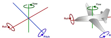
A test flight is conducted to analyze the active magnetism compensation caused by the aircraft and its components, such as engine accessories, engine masses, avionics, current generated on the fuselage, and other factors. It is tested in the project area and must include four selected headings (North, South, West, and East) or different headings based on the project. The test must include parallel control lines and pro-duction lines, according to the project guidelines. The sum of the anomalies in the area is received by the magnetome-ter when the aircraft performs control movements in all three axes. These control movements includes a±20◦roll (longi-tudinal), yaw±10◦(lateral, since it is centered in the vertical
Figure 10.Model of the aircraft maneuvers performed during the FOM test (source: modified from http://www.thevoredengineers. com/2012/05//the-quadcopter-basics, free domain).
axis), and±10◦pitch (vertical, since is around a horizontal axis). Figure 10 illustrates the three movement controls made in the FOM test. At altitudes of 3000 ft (914 m) or 4000 ft (1220 m), the incoming soil variations are typically low so that only the heading and maneuvers affect the test. The vari-ations are stored in the system and used for automatic com-pensation during future data acquisition projects (Hood and Ward, 1969).
If any change is made to aircraft equipment or any project parameters, a new FOM flight must be completed. Examples of the magnetic field by the components and the magnetic compensation are shown in the profiles of Fig. 11.
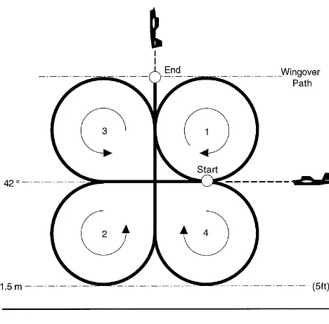
6.2 Clove-leaf
The clove-leaf flight test shows the degree of change experi-enced in the system when the aircraft changes heading during a data acquisition.
Generally, this variation should be zero. However, it can be stored and compensated for throughout the project.
The flight is conducted at specified height based on a planned heading and North–South or East–West directions (Fig. 12). After initial test flights, new headings can be deter-mined and flown via the same coordinates.
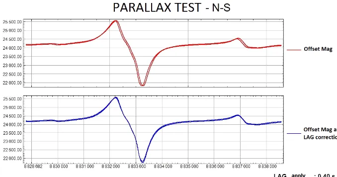
6.3 LAG
This flight test is used for measuring the magnetic field varia-tions in different acquisition direcvaria-tions using a magnetometer sensor. This test also utilizes radar altimeter measurements.
Generally, an anomalous region (magnetic and density) is selected to verify data along two acquisition headings, such as a hangar, ship, steel bridge, or a previously determined anomaly. The annotated acquisition time is taken into ac-count when performing the mapping. Results of the LAG test are shown in Fig. 13.
6.4 Altimeter radar
Figure 11.Example of magnetic field measurement interference caused by aircraft maneuvers (source: S. Guimarães, author private collec-tion, May 2007).
Figure 12.Maneuver model performed by the aircraft in the clove-leaf test (source: modified from https://www.ibiblio.org/hyperwar/ USN/ref/ASW-Convoy/ASW-Convoy-2.html, free domain).
The altimeter radar is important for data acquisition be-cause the elevation can directly interfere with concentrations count in certain situations. In addition, barometric equipment may change with pressure and temperature.
6.5 Drape
In mountainous regions, a drape (predetermined flight height) or relatively flat terrain is recommended for 3-D pro-cessing. This allows high mountain surface data to be more easily attained, superimposed, and mapped at a higher qual-ity. In this case, the height flown to acquire the control lines sets the production lines’ height. This method accounts for the aircraft performance in the flight environment. Each
air-craft climbs and descends at different rates based on size and other factors (Bryant et al., 1997). An example of drape is shown in Fig. 14.
6.6 Contour
Contour flights, often taken by helicopters, use the radar al-timeter for data acquisition and are best suited for flat land or sea (offshore). The pilot uses the radar altimeter to maintain a constant height of 91 m above the ground, reaching 150 m if towing a bird (Hood and Ward, 1969). On terrain with accen-tuated topographical variations, this process makes it difficult to maintain the predetermined altitude. Climbs and descents are based on the pilot’s experience, which is largely based on the craft, equipment, and terrain. Therefore, using multiple pilots for data acquisition will cause data inconsistencies and require manual correction.
7 Geophysical measurement corrections 7.1 Magnetic field
Magnetometric method corrections are necessary in the ac-quired measurements to isolate only the anomalous magnetic field of interest that, in this case, is the crust magnetic field. Therefore, observations are made during aerial acquisition of the total magnetic field (external and internal).
7.1.1 Diurnal magnetic monitoring – BaseMag
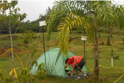
In general, diurnal magnetic monitoring (DMM) uses a ground magnetometer. This equipment is installed at a fixed position, called BaseMag, located as far as possible from magnetic interference. It is typically installed at the airport, at a location outside the predetermined interference, which aids in logistical measures and equipment security. Figure 15 shows the installation of BaseMag in operation.
Figure 13.LAG test results model applied to magnetic measurements (source: S. Guimarães, author private collection, May 2007).
field, which includes the main magnetic field (inside the Earth), external interference (magnetic variation of the sun due to interactions with solar winds), and the crustal mag-netic field.
These are ad hoc measurements, and in a magnetic interference-free area, the crustal magnetic field is negligi-ble. Therefore, the IGRF mathematical model can provide us with values related to the main magnetic field. Thus, mon-itoring must be conducted entirely outside the interference zone of the study area. Note that modern monitoring equip-ment has a range limit of 27 nautical miles (50 km), which is decreased during magnetic storms (Reeves, 2005). Figure 16 illustrates a geomagnetic field by BaseMag.
7.1.2 Magnetic anomalies in the surface
Magnetic anomalies are varied counts peaks. These peaks may be caused by railways, power lines, magnetic storms, large metallic masses, ships, buildings, and hangars. In addi-tion, anomalies can be caused by equipment aboard the air-craft that contains chemical substances, which may be de-tectable by the instrument (Hood and Ward, 1969).
These peaks are clearly observed in the data. However, they must not be confused with magnetic anomalies caused by the subsurface of interest. These peaks should be filtered and removed from the data sets.
7.1.3 Diurnal variations
During the day, the Earth is bombarded with charged mag-netic particles via solar winds. These loads compress from day to night and then expand, causing regular variations in the magnetic field. Nights are calmer for data acquisition, but more impractical in certain regions. These variations are monitored via Basemag.
7.1.4 Magnetic storm
Protons, electrons, and accelerated atomic particles are a re-sult of solar activity and are carried by solar winds, particu-larly during magnetic storms. These events can last for min-utes or hours and may reach 90 km h−1during geomagnetic storms. In some cases, the atmosphere may take days to sta-bilize. They have a larger influence at the Earth’s magnetic poles, affecting GNSS signal reception and radio electronic equipment. This causes major issues for data acquisition.
Weather monitoring equipment provides alerts for large storm events. Generally, monitoring data and forecasts from meteorological research centers shown are consulted prior to flights. The most common weather study centers are the tional Oceanic & Atmospheric Administration (NOAA), Na-tional Aeronautics and Space Administration (NASA), and their interagency branches.
8 Considerations related to geophysical flight
Flights require the extreme attention of the crew. In addition to flying the aircraft, the pilot must monitor instruments and navigate. The pilot must simultaneously note the relation of the aircraft to land, cities, airports, air traffic, animals, and other factors.
Normal flights follow predetermined standards, such as the acquisition speed needed to preserve data resolution. Exceed-ing this lateral limit (cross track) can cause an overlap of the perpendicular line, thus creating a gap on the map.
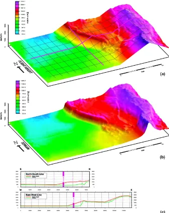
Figure 14. (a)Drape model applied to the acquisition and control lines,(b)topography of the terrain, and(c)results of an acquisition line flight with drape (source: (n.d.), http://www.terraquest.ca/wp-content/uploads/2014/05/surveycontours.jpg, last access: October 2014).
and cause the craft to tend to the right. This relationship is known as theP factor (Hurt Jr., 1965), which affects cross tracking. It is most noticeable in single-engine aircraft. The pilot should be alert to sudden power lever changes, which could lead to oversteering or overcompensation.
8.1 Line interception
The pilot may be given certain control lines to be flown. He may then consider the distances and degrees that allow the lines to be most efficiently flown, e.g., a line on the bow with an N–S curve to the right. It begins to curve 1.8 km away, with a stable tilt of 20 to cross the bow at 090. Note that 900 m is the distance at which the number is lower due to the curve. If it is greater, the pilot can choose to maintain or
decrease the ratio by a few degrees. When flying E–W head to cross bow 0 (360), a distance of 900 m is typically con-sidered. Figure 17 illustrates the flight plan with acquisition lines and tie lines.
8.2 Flight lines
Figure 15.Example of a day monitoring BaseMag station, which measures the magnetic field in parallel to an airborne geophysi-cal acquisition site (source: S. Guimarães, author private collection, January 2015).
Figure 16.Example of the diurnal magnetic field curve acquired at a BaseMag station (source: S. Guimarães, author private collection, May 2007).
8.3 Completing lines
Various lines or line segments may be flown successfully or unsuccessfully. These failures can include control lines or cross lines between control lines, which are the most notable lines due to their typically large flight distance.
9 Examples of results
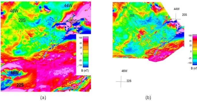
During airborne geophysical acquisitions, it is necessary to conduct data quality checks. In general, quality assessment and quality control (QA-QC) are conducted on all potential methods of geophysics and gamma spectrometry, which are limited by lateral offset and acquisition speed. Parameters that undergo QA-QC analyses include the magnetic field, temperature, spectrum range, and others. In addition, the acquisition area and control area are generally broken into grid blocks. Figure 18 illustrates the quality of two types of data acquisition. Figure 18a was measured during the 1980s, when measurement equipment was much less sophisticated.
Figure 17.Representation of the control and provisional acquisition lines (source: W. Urquhart, 2013, http://www.geoexplo.com/flight_ plan.gif, last access: October 2014, reprinted with permission as per email).
Figure 18b was measured in 2005, with 250 m line spacing and using the latest equipment. Both refer to the same area, located in the southern portion of the Minas Gerais state, Brazil.
Although a complete database was unavailable for Fig. 18b, the observed level of detail is much higher than in Fig. 18a. Note that developments in the airborne geo-physics field have led to exponentially improved data, in terms of both coverage and quality. These data have allowed for significant mineral exploration, geological studies, and geophysical analysis in Brazil and across the globe. For ex-ample, Fig. 19 illustrates a subsurface map of high-resolution aeromagnetic data, where the degree of certainty decreases as the data resolution increases.
Others studies show results of these evolution processes of the airborne data geophysical acquisition. A few examples in the scientific literature include Ravat (1996), LaBrecque and Ghidella (1997), Brozena et al. (2002, 2003), Finn and Morgan (2002), Salem and Ravat (2003), Hinze et al. (2005), Hemant et al. (2007), Bouligand et al. (2014), and Guimarães et al. (2014).
10 Final considerations
Figure 18. (a)Geophysical Brazil–Germany Project acquisition (code 1009 – CPRM, 1980) and(b)area second acquisition in 2005 (source: S. Guimarães, author private collection, November 2012).
exploration worldwide. This is thanks to improved magnetic field maps, radiometric, gravity and electromagnetic data, re-mote sensing, and other data collection and processing meth-ods.
This initial work was aimed at creating a summary of ac-quisition activities, including equipment and technical opera-tions used to enhance geophysical measurements and associ-ated results, as well as minimize problems encountered with these types of measurements.
Acknowledgements. We would like to thank Lev V. Eppelbaum for his immense support and all the colleagues that downloaded the material and commented during the discussion process.
Edited by: L. Eppelbaum
References
Airo, M. L.: Aeromagnetic and petrophysical investigations ap-plied to tectonic analisys in the northern Fennoscandian shield, Geol. Survey of Finland Report of Investigations 145, Geol. Sur-vey of Finland, Finland, p. 51, 1999.
Backus, G., Parker, R. L., and Constable, C.: Foundations of Geo-magnetism, Cambridge University Press, 369 pp., 1996. Barton, C.E., 1988. Global and regional geomagnetic reference
fields, Explor. Geophys., 19, 401–415, 1988.
Bouligand, C., Glen, J. M., and Blakely, R. J.: Distribution of buried hydrothermal alteration deduced from high resolution magnetic surveys in Yellowstone National Park, J. Geophy. Res.-Solid Ea., 119, 2595–2630, 2014.
Boyd, D.: The contribuition of airborne magnetic survey to geo-logical mapping, in: Minig and Groundwater Geophysics, 1967, Economic Geology Report 26, edited by: Morley, F., Geological survey of Canada, Ottawa, 213–227, 1970.
Brozena, J. M., Childers, V. A., Lawver, L. A., Forsberg, R., Faleide, J., and Eldholm, O.: A New Aerogeophysical Study of the Eura-sia Basin and Lomonosov Ridge: Implications for Basin Devel-opment, in: AGU Fall Meeting Abstracts, Vol. 1, p. 01, 2002. Brozena, J. M., Childers, V. A., Lawver, L. A., Gahagan, L. M.,
Forsberg, R., Faleide, J. I., and Eldholm, O.: New aerogeophys-ical study of the Eurasia Basin and Lomonosov Ridge: Implica-tions for basin development, Geology, 31, 825–828, 2003. Bryant, J., Coffin, B., Ferguson, S., and Imaray, M.: Horizontal and
vertical guidance for airborne geophysics, Can. Aeronaut. Space J., 43, 1–134, 1997.
Bullock, S. J. and Barrit, S. D.: Real-Time Navigation and Flight Path Recovery of Aerial Geophysical survey: A Review, Pro-ceedings of Ecploration ’87: Third Decennial International Con-ference on Geophysical and Geochemical Exploration for Min-erals and Groundwater, Ontario, 170–182, 1989.
Featherstone, W. E.: The Global Positioning System (GPS) and its use in geophysical exploration, Explor. Geophys., 26, 1–18, 1995.
Finn, C. A. and Morgan. L. A.: High-resolution aeromagnetic map-ping of volcanic terrain, Yellowstone National Park, J. Volcanol. Geoth. Res., 115.1, 207–231, 2002.
Guimarães, S. N. P., Ravat, D., and Hamza, V. M.: Combined use of the centroid and matched filtering spectral magnetic methods in determining thermomagnetic characteristics of the crust in the structural provinces of Central Brazil, Tectonophysics, 624–625, 87–99, 2014.
Hakli, P.: Practical test on accuracy and usability of Virtual Refer-ence Sation method in Finland, Anais FIG Working Week 2004, Athens, Greece, 2004.
Haugh, A.: DGPS, Doppler, datums and discrepancies – your posi-tions explained, First Break, 11, 485–488, 1993.
Hemant, K., Thébault, E., Mandea, M., Ravat, D., and Maus, S.: Magnetic anomaly map of the world: merging satellite, airborne, marine and ground-based magnetic data sets, Earth Planet. Sc. Lett., 260, 56–71, 2007.
Hildebrand, J. D.: Aerogeofísica no Brasil e a Evoluçaõ das Tec-nologias nos Últimos 50 anos, I Simpósio de Geofísica da SBGf, Brasil, 1–8, 2004.
Hinze, W. J., Aiken, C., Brozena, J., Coakley, B., Dater, D., Flana-gan, G. and Kucks, R.: New standards for reducing gravity data: The North American gravity database, Geophysics, 70, J25–J32, 2005.
Hjelt, S. E.: Experiences with automatic magnetic interpretation using the thick plate model, Geophys. Prospect., 21, 243–265, 1973.
Hood, P. and Ward, S. H.: Airborne Geophysical Methods, Adv. Geophys., 13, 1–112, 1969.
Hurt Jr., H. H.: NAVAIR 00-80T-80, aerodynamics for naval avia-tors, Naval Air Systems Command, University of Southern Cali-fornia, 293–294, 1965.
LaBrecque, J. L. and Ghidella, M. E.: Bathymetry, depth to mag-netic basement, and sediment thickness estimates from aerogeo-physical data over the western Weddell Basin, J. Geophys. Res.-Solid Ea., 102, 7929–7945, 1997.
Morrison, D.: Australian Society of Exploration Geophysicists, Pre-view Journal Issue, 109, 14 pp., 2004.
Packard, M. and Varian, R.: Free nuclear induction in the earth’s magnetic field, in: Physical Review, One Physics Ellipse, Amer-ican Physical Soc., MD, USA, 941–941, 1954.
Parkinson, W. D.: Introduction to Geomagnetism, Scottish Aca-demic Press, Edinburg, 433 pp., 1983.
Puranen, M. and Puranen, R.: Apparatus for the measurement of magnetic susceptibility and its anisotropy, Report of Investiga-tion 28, Geological Survey of Finland, Espoo, 46 pp., 1977. Ravat, D.: Analysis of the Euler method and its applicability in