Frequency domain analysis of transient flow in pipelines; application of the genetic programming to reduce the linearization errors

(1)

SUMMER 2018, Vol 4, Issue 1, JOURNAL OF HYDRAULIC STRUCTURES Shahid Chamran University of Ahvaz

Journal of Hydraulic Structures J. Hydraul. Struct., 2018; 4(1): 75-90

DOI: 10.22055/JHS.2018.25596.1073

Frequency domain analysis of transient flow in pipelines;

application of the genetic programming to reduce the

linearization errors

Mohammad Mehdi Riyahi1 Mostafa Rahmanshahi2

Mohammad Hadi Ranginkman3

Abstract

The transient flow analyzing by the frequency domain method (FDM) is computationally much faster than the method of characteristic (MOC) in the time domain. The FDM needs no discretization in time and space, but requires the linearization of governing equations and boundary conditions. Hence, the FDM is only valid for small perturbations in which the system’s hydraulics is almost linear. In this study, the linearization errors of the FDM applied to a reservoir-pipe-valve system (RPV) are discussed and by using the Genetic Programming (GP), some correction coefficients are defined to reduce them. By applying the correction coefficient at the opening size of the valve, the first frequency of the frequency domain method is modified. Moreover, the responses at higher-order frequencies are evaluated by some new correction factors obtained by the GP. Solving an illustrative example shows that the error of the system can be significantly reduced by using the applied correction factors.

Keywords:Frequency domain, Transient flow, Method of characteristics, Genetic programming

Received: 22 March 2018; Accepted: 08 May 2018

1. Introduction

In addition to the traditional solution for solving the transient flow governing equations in pipelines by using the numerical methods such as the method of characteristic [1], the characteristics wave method [2], the finite element method [3], and the finite differences method [1]; they can also be solved by the transfer matrix method [4] and the impedance method [5] in

1_{M.Sc. graduated, Department of Civil Engineering, Shahid Chamran University of Ahvaz, Ahvaz, Iran,}

[email protected] (Corresponding author)

2_{Ph.D. graduated, Department of Water Science Engineering, Shahid Chamran University of Ahvaz,}

Ahvaz, Iran, [email protected]

3_{Ph.D. graduated, Department of Civil Engineering, Shahid Chamran University of Ahvaz, Ahvaz, Iran,}

(2)

the frequency domain. The numerical methods in time domain need for discretization of the problem into the time and space and this increases the time of computations. While, in the frequency domain method since there is no need for discretization, the speed transit flow analysis is much higher than the time-domain numerical methods. This problem becomes more serious when a system has a complex mesh or needs to be connected to an optimization model. Another advantage of the frequency domain analysis is that the output of the frequency response function (FRF) does not depend on the type of the system excitation [6]. By applying different types of the excitations to a piping system in the time domain, the pressure head signal will result in different shapes. However, if the Fourier transform of the pressure head signal is taken and divided by the Fourier transform of the applied excitation, the FRF is obtained, which does not depend on the type of excitation. Compared to the characteristics method, the linearization of governing equations and boundary conditions in the frequency domain method (FDM) leads to creating errors in the output of this method. Nowadays the frequency domain is used for analyzing the water hammer phenomena [7-9], leak detection [10-12], and blockage detection [13, 14] is spread like the time domain[15] . Despite many conducted studies using the frequency domain a few studies have been carried out on the error of the frequency domain [16-19].

Lee et al. [16] showed that by increasing the valve opening size during the excitation, the system does not act as linear system and the linearization errors are increased. Lee and Vítkovský [17] introduced the dimensionless parameter, k, which was a criterion for measurement of the head loss at the valve, by dividing a pipe system into two states of friction dominant and valve dominant. For large values of k, the state of the valve is called valve dominant and for small k values, it is called the friction dominant. They represented that for the small values of k, the frequency response method (FRM) showed larger values compared to the method of characteristics, and when k has larger values, the FRM showed smaller values than the method of characteristics. They also investigated the generated errors between the characteristics method and the FRM by using a reservoir- pipe- valve (RPV) system. They indicated that in the openings less than 20%, the system did not show too many errors.

Lee [18] demonstrated that in the small excitations using a RPV system, the obtained values from using the transmission line model and characteristics model are similar. By increasing the magnitude of valve excitation, the created errors between the transmission line model and the characteristics model increases. Additionally, this paper demonstrates that the output of the transfer linear model has only one frequency, while the output of the characteristics model has the highest frequencies, causing a difference in the pressure head output at the time domain between two models. In this paper, the energy phase diagram was used to assess the created errors between the transfer linear model and characteristics model.

Riyahi and Haghighi [19] transmitted the linear equations of the frequency domain to the time domain; they replaced these equations in the MOC and compared them with the outputs of the frequency and full nonlinear MOC. It was concluded that the effect of the linearity or nonlinearity of the steady friction term in the frequency domain output is negligible and the main source of the error is the linear term of the valve equation. In addition, they showed that calibration in the frequency domain, unlike time domain, cannot be done with steady friction term; instead, it can be done with reforming of valve opening rate.

(3)

frequencies. Finally, the generality of the proposed modifications is evaluated through solving several different examples and the results are discussed.

2. Governing Equations and Valve Equation

2.1. Governing Equations

For analyzing the transient flow in pipelines, the governing equations must be solved. In many engineering problems, the governing equations on transient flows in elastic pipelines are as follows [20]:

( 1 ) 𝜕𝑄 𝜕𝑡 + 𝑔𝐴 𝜕𝐻 𝜕𝑥 + 𝑓𝑄|𝑄|

2𝐷𝐴 = 0

(2) 𝜕𝐻 𝜕𝑡 + 𝑎2 𝑔𝐴 𝜕𝑄 𝜕𝑥 = 0

where, 𝑄 is the discharge, 𝐻 is the pressure head, 𝑔 is the gravitational acceleration, 𝐴 is the pipe cross-section area, 𝐷 is the pipe diameter, 𝑓 is the Darcy-Weisbach factor, and 𝑥 is the location in pipe length.

There are two methods for the analysis of transient flows in the frequency domain; the transfer matrix method and the impedance method. In this study, the transfer matrix method is used, in order to maintain simplicity and easy understanding. In the transfer matrix method, the pressure head and discharge at the upstream and downstream of the system are related to each other through the transfer matrix.

The produced flows in the frequency domain are considered as oscillatory steady flows; therefore, in order to solve the governing equations on the transient flows in pipelines at the frequency domain, firstly, it must be assumed that the discharge, pressure head, and valve opening are equal to the average values plus their fluctuation values.

(3)

𝑄 = 𝑄0+ 𝑞∗

(4)

𝐻 = 𝐻0+ ℎ∗

( 5 )

𝜏 = 𝜏0+ 𝜏∗

where, 𝑄0, 𝐻0, and 𝜏0 represent the average values and 𝑞∗, ℎ∗ and 𝜏∗ are the fluctuation

values around the average value.

Now, by substituting Eqs. (3) to (5) into Eqs. (1) and (2), and eliminating the non-linear term of the momentum equation, the following equation is obtained.

(6) 𝜕𝑞∗ 𝜕𝑥 + 𝑔𝐴 𝑎2 𝜕ℎ∗

𝜕𝑥 = 0

( 7 ) 𝜕ℎ∗ 𝜕𝑥 + 1 𝑔𝐴 𝜕𝑞∗ 𝜕𝑡 + 𝑓𝑄₀

𝑔𝐷𝐴2𝑞∗= 0

(4)

(8)

𝜕𝑞 𝜕𝑥+

𝑔𝐴

𝑎2ℎ𝑗𝜔 = 0

( 9 ) 𝜕ℎ 𝜕𝑥+ 1 𝑔𝐴𝑞𝑗𝜔 + 𝑓𝑄0

𝑔𝐷𝐴2𝑞 = 0

where, q and h are the Fourier transform of 𝑞∗ and ℎ∗ values. Also, 𝜔 is the angular frequency and 𝑗 = √−1. By solving Eqs. (8) and (9), the following equations are obtained:

(10)

𝑞𝐷= −

ℎ_𝑈

𝑍𝑐sinh(𝜇𝑥) + 𝑞𝑈cosh (𝜇𝑥)

(11)

ℎ_𝐷= −𝑍_𝑐𝑞_𝑈sinh(𝜇𝑥) + ℎ_𝑈cosh (𝜇𝑥)

(12) 𝑧𝑐 = (𝜇𝑎 2₎ (𝑗𝜔𝑔𝐴) ⁄ ( 13 )

𝜇2₌𝑎𝐴𝑗𝜔

𝑎2 (

𝑗𝜔 𝑔𝐴+

𝑓𝑄₀ 𝑔𝐷𝐴2)

where, 𝑍𝑐 and 𝜇 are called the characteristic impedance and the propagation constant,

respectively. The subscripts U and D are also referred to as the upstream and downstream of the pipe, respectively. Thus, the field matrix with respect of Eqs. (10) to (13) can be written as follows:

(14)

F = [ cosh (𝜇𝑥) −

1

𝑍_𝑐sinh(𝜇𝑥) 0

−𝑍𝑐sinh(𝜇𝑥) cosh (𝜇𝑥) 0

0 0 1

]

2.2. Valve Equation

The valve equation can be written as follows [4]:

(

15

)

𝑄 𝑄0=

𝐶_𝑑𝐴 (𝐶𝑑𝐴)0(

𝐻 𝐻0)

1 2 ⁄

in which, 𝐶𝑑 is the coefficient of discharge and (𝐶𝑑𝐴)0 , 𝐶𝑑𝐴 are equal 𝜏0 and 𝜏, respectively.

By replacing Eqs. (6) and (7) into the Eq. (15), the following equation can be achieved:

(

16

)

(1 + 𝑞

∗

𝑄₀) = (1 + 𝜏∗

𝜏₀) (1 + ℎ∗

𝐻₀)

1 2 ⁄

The Expression (1 +ℎ ∗

𝐻0)

1 2 ⁄

(5)

(

17

)

(1 + 𝑞

∗

𝑄0) = (1 +

𝜏∗

𝜏0) (1 +

ℎ∗

𝐻0) 1

2 ⁄

=

(1 +𝜏

∗

𝜏)(1 + 1 2

ℎ∗

𝐻0−

1 8(

ℎ∗

𝐻0) 2

+ 3

48( ℎ∗

𝐻₀)

2

+ ⋯ )

With removing the non-linear terms in Eq. (17), the following equation is obtained.

(

18

)

(1 +𝑞∗

𝑄0) = 1 + (

𝜏∗

𝜏0) + (

1 2

ℎ∗

𝐻0 )

By applying the Fourier transform in Eq. (18), the following equation can be achieved:

(

19

)

ℎ −2𝐻0 𝑄0 𝑞 +

2𝐻₀∆𝜏 𝜏0 = 0

in which, ∆𝜏 indicates the Fourier transform of 𝜏∗ and equals to maximum valve opening. The point matrix can be written using Eq. (19), as follows:

(

20

)

P = [−

1 0 0

2𝐻0

𝑄0 1

2𝐻0∆𝜏

𝜏0

0 0 1

]

2.3. Overall Matrix

The overall matrix can be achieved by multiplying the point matrix to the field matrix. Accordingly, by multiplying Eq. (20) in Eq. (14), the overall matrix can be obtained, as follows:

(21)

𝑈 = [−

1 0 0

2𝐻0

𝑄0 1

2𝐻0∆𝜏

𝜏0

0 0 1

] [ cosh (𝜇𝑥) − 1

𝑍𝑐sinh(𝜇𝑥) 0

0 0 1

]

3. Genetic Programming

(6)

of a system is unknown, and (c) Grey box: they are conceptual systems that create a mathematical relationship between inputs and outputs of a system and make it available for the users. According to the above-mentioned categories, GP and ANNs are considered as the grey and black categories, respectively.

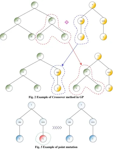
GP is an evolutionary computation method which solves the problem without knowing the solution and/or recognition of it by the user [26]. GP is derived from the genetic algorithm (GA) method and treats according to the genetic rules. This model was first discovered by Carmer [27]; then developed by Koza [28]. The difference between the GA and GP method is that the GA method is used to find the best value for a series of parameters for the model, while the GP provides a structure to associate the input data to the output data [23]. In fact, the GA optimizes the parameters, whereas the GP performs the modelling. In GPfirstly, a population from the computer programs is generated using one of the three, full, Growing, and ramped half-and-half methods. A program, which is formed in the GP method, consists of two main parts, terminals and functions. The terminals include non-numeric and numeric variables and the functions include mathematical operators and functions, Boolean operators, and logical expressions. The output of a program can be illustrated like a tree (Fig. 1). Functions and terminals have been shown in the Fig. 1. Functions are placed in the middle points and terminals in the branches.

Fig. 1 GP structure

(7)

shown in Fig. 3. In the reproduction method, a program is selected based on fitness and it is transferred to the next generation.After creating the new generation, the same cycle as described above is repeated until the number of iterations is finished; then, the best program among the available programs is selected in accordance with fitness.

Fig. 2 Example of Crossover method in GP

(8)

4. Reducing Error with Genetic Programming

In this research, as shown in Fig. 4, a simple RPV system was used. This system is consists of a reservoir with 50 m head at its upstream, a pipe with 1000 m length, 250 mm diameter, Darcy friction factor of 0.021 and wave speed of 1000 ms-1. The excitation is produced by the valve which is sinusoidal excited and is located at the end of RPV system.

Fig. 4 Reservoir-Pipe-Valve system

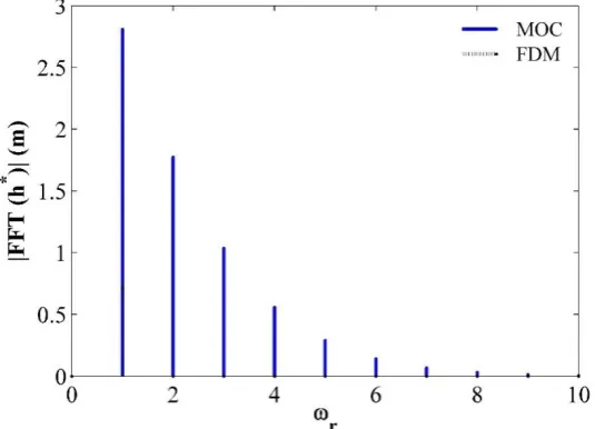
The results of the FDM have been compared with the results of the MOC in Fig. 5, using the provided system in Fig. 4. In this system, the valve has been excited sinusoidal with the theoretical frequency of the system fthr which is equal to a⁄_4L and 𝐶𝑑 is 0.8. The results

have been compared at the location of the valve and the Fast Fourier Transformation (FFT) has been used for transferring the obtained pressure heads from the characteristic method to the frequency domain. Fig. 5 indicates, that the frequency domain only produces the first frequency which is not equal to the output of the characteristic method, due to the large excitation of the valve. Thus, the FDM needs to produce and correct higher-order frequencies in addition to the correction of the first frequency.

Fig. 5 Comparison of the responses between MOC & FDM

(9)

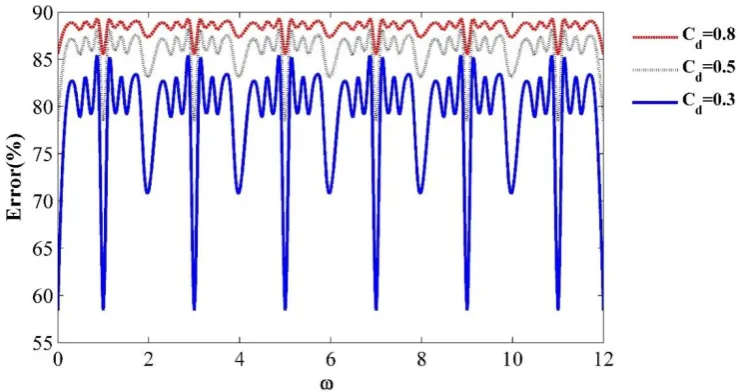
obtained for frequencies 1 to 12 and discharge coefficients 0.3, 0.5, and 0.8 (Fig. 6). Consequently, the corrections can be made for a frequency interval and the other frequencies can also be corrected by the similar corrected frequencies. In this research, the frequency intervals ranging from 1 to 3 have been corrected.

Fig. 6 The linearization error of the FDM for 𝝎𝒓 from 0 to 12 and coefficient of discharge 0.3, 0.5

and 0.8

For correction of the output frequencies, a correction coefficient (𝛼) is multiplied to the valve opening. Since, the correction coefficient is considered in the valve relationships in the transfer matrix method; as a result, the point matrix is changed, and it can be rewritten as follows:

( 22 )

P = [−

1 0 0

2𝐻₀

𝑄₀ 1

2𝛼𝐻₀∆𝜏 𝜏₀

0 0 1

]

Due to the changes in the point matrix, the overall matrix is also changed. The overall matrix can be rewritten as follows.

(23)

𝑈 = [−

1 0 0

2𝐻0

𝑄0 1

2𝛼𝐻0∆𝜏

𝜏0

0 0 1

] [ cosh (𝜇𝑥) − 1

𝑍𝑐sinh(𝜇𝑥) 0

0 0 1

]

According to Eqs. (22) and (23), when the correction coefficient equals 1, the same equations described before, are achieved. The following steps are considered for computing the value of α,. The relevant flowchart is represented in Fig. 7;

a) First, the MOC is applied to the situation that the valve is excited sinusoidal with a specific frequency, a given opening size and discharge coefficient.

(10)

c) Then, each obtained amplitude at each output frequency is set equal to the output of the FDM.

d) The value of q is calculated by the following formula. Notice that the value of h has been calculated from the previous step.

( 24 )

𝑞 = ℎ

−𝑍_𝐶sinh (𝜇𝑥)

e) The value of α is calculated as follows:

( 25 )

𝛼 = 𝑞 (−𝑍𝐶 sinh(𝜇𝑥) −2𝐻_𝑄0

0 cosh(𝜇𝑥)) (

−𝜏0

2𝐻0∆𝜏)

The value of α has been calculated for the values of ∆τ and 𝐶𝑑 from 0.1 to 0.8 and values of ω

from 1 to 3. Then, the data has been divided into two categories of training and test data; afterwards, using the GP method, four equations have been achieved for α based on the input and output frequency, valve opening, and discharge coefficient, these equations are 𝛼₁, 𝛼₂, 𝛼₃and

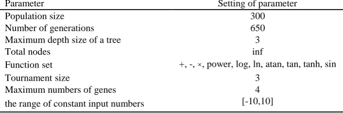
𝛼₄ which are related to the first frequency, frequencies 2 and 3, frequencies 4 to 6 and frequencies 7 to 10, respectively. The determined parameters in the GP method are expressed in Table 1:

Table1. The determined parametersin the GP method

Parameter Setting of parameter

Population size 300

Number of generations 650

Maximum depth size of a tree 3

Total nodes inf

Function set +, -, ×, power, log, ln, atan, tan, tanh, sin

Tournament size 3

Maximum numbers of genes 4

the range of constant input numbers [-10,10]

(11)

In this study, the GP is implemented by means of MATLAB toolbox (GPTIPS2).[29, 30] The equations for the correction coefficients, α, are given as follows. Moreover, the values of determination coefficient for each equation are 0.94, 0.95, 0.93, and 0.90, respectively.

𝛼₁= 12.5 ∗ sin(∆𝜏4.3_{∗ tan(𝐶}

𝑑)) − 0.93 ∗ sin(atan(𝐶𝑑)atan(𝜔𝑖𝑛)) + 1.62

)

26

(

𝛼₂ = 5.4 ∗ tan(tan (∆𝜏)) ∗ tanh(tanh(𝐶_𝑑)) − 4.63 ∗ tan(∆𝜏) ∗ tanh(𝐶𝑑) − 1.5

∗ log (𝜔𝑜𝑢𝑡)tan (tanh (∆𝜏)+ 1.56

)

27

(

𝛼₃ = 7.4 ∗ 𝑥12∗𝜔𝑜𝑢𝑡atan(𝐶

𝑑) + 0.66 ∗ tanh(∆𝜏)𝜔𝑜𝑢𝑡− 2exp (−3)

)

28

(

𝛼4 = 10.7 ∗ ∆𝜏2∗𝜔𝑜𝑢𝑡∗ log(𝜔𝑜𝑢𝑡) ∗ sin(𝐶𝑑) − 2.81 ∗ ∆𝜏 ∗ 𝑥12∗𝜔𝑜𝑢𝑡𝜔𝑜𝑢𝑡∗ sin(𝐶𝑑)

+ 6.15 ∗ 10−4

)

29

(

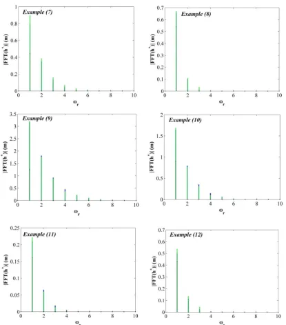
5. Examples

To investigate the efficiency of the obtained correction coefficients and their generality in different situations the provided systems in Table 2 have been used. In these examples, the systems with different properties like the length, wave speed, Darcy- Weisbach factor have been used that are presented in Table 2. In all examples, oscillatory-state flows are generated by sinusoidal exciting the vale.

Each system is implemented one time using the MOC, then the obtained fluctuations of the pressure head are transferred into the frequency domain by the FFT. The pressure head amplitudes obtained by the MOC are adopted as the exact solutions. After that, each system has been implemented by the standard FDM (SFDM) and modified FDM (MFDM). Finally, the results of the SFDM and MFDM are compared with MOC.

Table 2. Examples of the RPV systems

As earlier discussed, the system’s nonlinearities not only cause the FRM to under predict or over predict the system response at the excitation frequency but also produces responses at higher-order frequencies which are completely missed by the SFRM. In this research with introducing correction factor that is named 𝛼1 can reform the first frequency of SFDM. To

generate higher-order frequencies, these frequencies are made like the first frequency. Then by applying correction coefficients that are named 𝛼₂, 𝛼₃and 𝛼₄ they can be approximated to their

Example a (m/s) d (m) L (m) f Hup (m) Cd 𝜔𝑟 ∆𝜏

1 1000 0.25 1000 0.021 50 1 1 0.8

2 1200 0.4 1000 0.022 10 1 2.5 0.8

3 800 0.3 800 0.02 20 0.5 1.5 0.5

4 1000 0.45 1000 0.02 30 0.8 2 0.6

5 1200 0.25 1200 0.022 50 0.3 2.5 0.3

6 1100 0.25 900 0.022 10 0.3 1 0.8

7 1200 0.35 800 0.022 40 1 2 0.6

8 1000 0.15 1000 0.02 20 0.2 2.5 0.2

9 800 0.25 900 0.02 35 0.5 1.4 0.7

10 1000 0.2 800 0.021 22 0.4 2.3 0.6

11 1200 0.1 600 0.018 40 0.95 1.7 0.4

(12)

actual values. The output of SFDM, MFDM and MOC are shown in Fig. 8.

Table 3 represents the errors between the MOC and the SFDM, as well as the errors between the MOC and the MFDM for the first frequency output. This table shows a significant reduction in errors by applying correction coefficients in the SFDM.

Table 3. Error between MOC and SFDM and also MOC and MFDM in the first frequency output

6. Conclusion

Despite the advantages of the FDM, such as fast computations and providing more insight towards the system, it suffers from a big limitation that is the linearization of the non-linear equations. Linearization causes this method to only have an exact response for small excitations and when the system loses its linearization state, it is not able to make accurate predictions. Furthermore, this method is not capable to produce higher-order frequencies. Despite increasing the application growth of the frequency domain in water engineering; Althogh currently, there are few investigations on reducing the frequency domain errors. In this study, by using GP which has been one of the most widely used tools in the recent years in various fields such as water engineering, it is possible to correct the response output of the frequency domain for the first frequency and for higher frequencies, they can be corrected after producing each of them. This correction coefficient depends on the input and output frequencies, valve opening, and discharge coefficient. The coefficient obtained from GP is multiplied to the valve opening; then by correcting the relevant output, the FRM is improved. In accordance with the mentioned examples, in the worst situation, the error value of the first frequency has decreased from 76.98 to 0.3 %.

Example Error between MOC & SFDM (𝜔1) Error between MOC & MFDM (𝜔1)

1 75.67 6.06

2 76.99 0.3

3 33.69 4.16

4 41.29 16.74

5 19.38 3.26

6 59.72 25.59

7 44.64 11.98

8 17.73 1.65

9 60.16 0.016

10 45.32 2.47

11 23.27 5.16

(13)

(14)

Fig. 8 Responses of the examples in the frequency domain

References

1. Izquierdo J, Iglesias P, (2002). Mathematical modelling of hydraulic transients in simple systems. Mathematical and Computer Modelling, pp: 801-812.

2. Wood D.J, et al., (2005). Numerical methods for modeling transient flow in distribution systems. Journal (American Water Works Association), pp: 104-115.

3. Zhao M, Ghidaoui MS, (2004). Godunov-type solutions for water hammer flows. Journal of Hydraulic Engineering, pp: 341-348.

(15)

5. Wylie E.B., Streeter V.L., and Suo L., Fluid transients in systems. Prentice Hall Englewood Cliffs, NJ, Vol. 1. 1993.

6. Lee P.J, et al., (2013). Frequency domain analysis of pipe fluid transient behaviour. Journal of hydraulic research, pp: 609-622.

7. Kim S.-H., (2010). Design of surge tank for water supply systems using the impulse response method with the GA algorithm. Journal of Mechanical Science and Technology, pp: 629-636. 8. Ranginkaman MH, Haghighi A, and Samani H.M.V, (2017). Application of the Frequency

Response Method for Transient Flow Analysis of Looped Pipe Networks. International Journal of Civil Engineering, pp: 677-687.

9. Riasi A, Nourbakhsh A, and Raisee M, (2010). Numerical modeling for hydraulic resonance in hydropower systems using impulse response. Journal of Hydraulic Engineering, pp. 929-934.

10. Capponi C, et al., (2017). Leak Detection in a Branched System by Inverse Transient Analysis with the Admittance Matrix Method. Water Resources Management, pp: 1-15. 11. Ferrante M, et al., (2016). Numerical transient analysis of random leakage in time and

frequency domains. Civil Engineering and Environmental Systems, pp: 70-84.

12. Ranginkaman M, Haghighi A, and Vali Samani H, (2016). Inverse frequency response analysis for pipelines leak detection using the particle swarm optimization. Iran University of Science & Technology, pp: 1-12.

13. Duan H, et al., (2014). Transient wave-blockage interaction and extended blockage detection in elastic water pipelines. Journal of fluids and structures, pp: 2-16.

14. Duan H.-F., et al., (2013). Extended blockage detection in pipes using the system frequency response: analytical analysis and experimental verification. Journal of Hydraulic Engineering, pp: 763-771.

15. Bergant A, et al., (2013). Waterhammer tests in a long PVC pipeline with short steel end sections. Journal of Hydraulic Structures, pp: 24-36.

16. Lee PJ, et al., (2003). Leak detection in pipes by frequency response method using a step excitation: By WITNESS MPESHA, M. HANIF CHAUDHRY, and SARAH L. GASSMAN, Journal of Hydraulic Research, pp: 55-62.

17. Lee PJ, and Vítkovský JP, (2010). Quantifying linearization error when modeling fluid pipeline transients using the frequency response method. Journal of Hydraulic Engineering, pp: 831-836.

18. Lee, PJ, (2013). Energy analysis for the illustration of inaccuracies in the linear modelling of pipe fluid transients. Journal of Hydraulic Research, pp: 133-144.

19. Riyahi M.M, Haghighi A, (2018). Investigation of error resources in the transient flow simulation of pipelines in the frequency domain using the transfer matrix method, Modares Mechanical Engineering, pp: 10-18 (in Persian).

20. Ghidaoui M.S, et al., (2005).A review of water hammer theory and practice. Applied Mechanics Reviews, pp: 49.

21. Bozorg-Haddad O, Soleimani S, and Loáiciga HA, (2017). Modeling Water-Quality

Parameters Using Genetic Algorithm–Least Squares Support Vector Regression and Genetic Programming. Journal of Environmental Engineering, pp: 04017021.

22. Pourzangbar A, et al., (2017). Predicting scour depth at seawalls using GP and ANNs. Journal of Hydroinformatics, pp: 349-363.

(16)

24. Flood I, (2008). Towards the next generation of artificial neural networks for civil engineering. Advanced Engineering Informatics, pp: 4-14.

25. Giustolisi O, et al., (2007). A multi-model approach to analysis of environmental phenomena. Environmental Modelling & Software, pp: 674-682.

26. Poli R, Langdon W, and McPhee N, (2008). A field guide to genetic programming (With contributions by JR Koza). Published via http://lulu.com .

27. Cramer N.L., A representation for the adaptive generation of simple sequential programs. in Proceedings of the first international conference on genetic algorithms. 1985.

28. Koza J.R., Genetic programming: on the programming of computers by means of natural selection, MIT press, 1992.

29. Searson D.P., Leahy D.E. Willis M.J. (2010). GPTIPS: an open source genetic programming toolbox for multigene symbolic regression. in Proceedings of the International multiconference of engineers and computer scientists.