White Noise Path Integral Evaluation of the Characteristic Function of a Modified Wormlike Chain

(1)

White Noise Path Integral

Evaluation of the Characteristic Function

of a Modified Wormlike Chain

1_{Karl Patrick S. Casas and}2_{Jinky B. Bornales} 1_{Cebu Normal University}2_MSU-IIT

Date Submitted: May 25, 2011 Date Revised: July 5, 2011

ABSTRACT

The characteristic function of a wormlike chain is expressed as a Feynman path integral, obtained via the white noise functional approach. In order to describe the model statistically, the following physical assumptions are considered: (i) the wormlike chain curve is analogous to a trajectory of a quantum particle, and (ii) the total contour length L of the Wormlike chain is regarded as “time” t. The mathematical treatment is then facilitated by modifying its “Lagrangian”, given by Fixman and Kovac, wherein the resulting expression of the “Lagrangian” is just similar to the harmonic oscillator in an external electric field. Then, the cosine of the angle between the field vector and the tangent vector is approximated. In order to evaluate the characteristic function in one dimension only, we let this angle be linearly dependent on the contour distance of the chain. The characteristic function is then evaluated via white noise analysis. The result, with the field set to zero, is then compared to a propagator of a harmonic oscillator in an inverse potential.

Keywords: wormlike chain, white noise analysis, lagrangian, harmonic

INTRODUCTION

There has been a vast literature on different models in order to formulate functional integrals related to the statistics of stiff chains. One of these models is the Kratky-Porod wormlike chain model or simply the wormlike chain (WLC) model. This model envisions a homogeneous, isotropic, continuous flexible rod which makes this model the standard model for semiflexible and stiff polymers(Yamakawa, 1976, Taute et al., 2008, Marko et al., 1995).

However, the mathematical treatment is difficult, and one cannot possibly arrive at the expression of the characteristic function in its closed form. Therefore, various modifications must be done. To be able to do that, a physical assumption is considered: the wormlike chain is analogous to a trajectory of a quantum particle, so that the characteristic function can then be expressed in terms of the Feynman path integral. The modifications are then based on its CNU Journal of Higher Education

Volume 5, 2011, p. 19-26

1_{Cebu Normal University}

2_{Mindanao State University-Iligan Institute of Technology}

White Noise Path Integral

Evaluation of the Characteristic Function

of a Modified Wormlike Chain

1_{Karl Patrick S. Casas and}2_{Jinky B. Bornales} 1_{Cebu Normal University}2_MSU-IIT

Date Submitted: May 25, 2011 Date Revised: July 5, 2011

ABSTRACT

The characteristic function of a wormlike chain is expressed as a Feynman path integral, obtained via the white noise functional approach. In order to describe the model statistically, the following physical assumptions are considered: (i) the wormlike chain curve is analogous to a trajectory of a quantum particle, and (ii) the total contour length L of the Wormlike chain is regarded as “time” t. The mathematical treatment is then facilitated by modifying its “Lagrangian”, given by Fixman and Kovac, wherein the resulting expression of the “Lagrangian” is just similar to the harmonic oscillator in an external electric field. Then, the cosine of the angle between the field vector and the tangent vector is approximated. In order to evaluate the characteristic function in one dimension only, we let this angle be linearly dependent on the contour distance of the chain. The characteristic function is then evaluated via white noise analysis. The result, with the field set to zero, is then compared to a propagator of a harmonic oscillator in an inverse potential.

Keywords: wormlike chain, white noise analysis, lagrangian, harmonic

INTRODUCTION

There has been a vast literature on different models in order to formulate functional integrals related to the statistics of stiff chains. One of these models is the Kratky-Porod wormlike chain model or simply the wormlike chain (WLC) model. This model envisions a homogeneous, isotropic, continuous flexible rod which makes this model the standard model for semiflexible and stiff polymers(Yamakawa, 1976, Taute et al., 2008, Marko et al., 1995).

(2)

“Lagrangian”. These modifications arise to different models of different authors which are summarized by H. Yamakawa. Among the models discussed, the Fixman and Kovac (FK) model has a considerable result in which its Fokker-Planck equation is just similar to the Schrodinger equation of a harmonic oscillator in a uniform field. This model also has permitted stretching in the polymer chain and it is still valid for both flexible and rigid limits. Thus, this model reflects a physical property of the polymer. In this paper, the characteristic function of the FK model is obtained via the Hida and Streit formulation of the Feynman path integral where we assume that the chain has observable bending.

The Wormlike Chain, Model

In this section, a brief review of the wormlike chain model as discussed in the paper by H. Yamakawa is presented.

u�s� � ��_�� (1)

We note that,

u�_{� �,} ₍₂₎

and so u is a unit vector. The end-to-end distance is defined as _{R � � u��}_�L , integrated from one end to the other end of the polymer. If � �� , the mean square end-to-end distance_�R�_{� � �� }�_{, and if}_{�� , �R}�_{� � ��}_{. Thus, the} Kratky-Porod chain can interpolate to both extremes, random and rigid coil.

From Eqs. (1) and (2), one can obtain a relation, ��∆u��_{� � � � ∆�}_which tells us that the generation of the curve can be described by a Markov process, which implies that the distribution function satisfies the Fokker-Planck equation. Its Fourier transform is given by (Yamakawa, 1976)

�_�� u� � ��, u��u�� u � u��. (3) where � ��, u��u�� is the characteristic function and also the Green’s function. Note that Eq.(3) is just similar to the Schrodinger equation of a free particle with an external field k.

Now, there is a close analogy between the wormlike chain and a quantal trajectory of a particle, the chain contour length being regarded as “time”. Thus, the unnormalized characteristic function � ��, u��u�� may be written in the form,

(3)

where L is the “Lagrangian” (in units of h),

� �_�� _�� · u, (5)

subject to the condition given by Eq.(2).

Modified Wormlike Chain: Fixman and Kovac (FK) Model

Since it is impossible to find the exact solution of Eq.(3) thus, for

mathematical reasons, there is a need to relax the constraint given in Eq.(2) and the “Lagrangian” must be modified to

� ��_��_�� · u, (6)

where U is an additional true potential associated with the relaxation of the constraint, so that -(iU+k·u) is the “potential energy” of the “particle” and the bending constant _{�� }��_{. Then, eq. (3) takes the form,}

�_�� _� �

�_{� �� · u� � �� u��u}

�� u � u��, (7)

where V is determinable from U.

Depending on the system considered, the expression for U may vary for different models. For the Fixman and Kovac model, the potential is given by �� _{� �}�� _��

�� u. In this case, the characteristic function given in

Eq.(4) is just the path integral expression for a harmonic oscillator in an external force field k-if.

White Noise Path integration of the Characteristic Function

In this section, the evaluation of Eq.(4), with

� ��_��_��

� �� · u, (8)

in the language of white noise analysis is presented. To illustrate the use of white noise analysis, the simple case where the angle between the “field” and the tangent vector, u(s), is very very small, i.e., �� , is considered. The evaluation can be done by first employing a change of variable _{� � � �}��

�� so

that,

� ��_��_��

� �

��

�� (9)

(4)

Consider now the exponential in Eq.(4) with Eq.(9),

exp�� exp �� _��_��

� �

��

�� . (10) The paths U(s) of the Lagrangian must be parametrized by introducing trajectories of U consisting of a sure path _�� plus a Brownian (Streit et al., 1983) fluctuation,

�� _�� , (11)

where _{� � � ��} is the Brownian motion and _� is the white noise variable. With the parametrization in Eq.(11), the first term in Eq.(10) results in

exp �� _� ��_{� � exp��}_ω_,_ω_��_. ₍₁₂₎

Note that using the parametrization in Eq.(11), the second term in Eq.(10), depends at most quadratically on Brownian motion, B(s). By expanding it in terms of Taylor series and setting the initial point _�� _{� �}one can express _{��} (Streit et al., 1983) as

�� _��, ��′′�� (13)

where ��′′�� _�� ′′�� and �′′� �. To be able to express the characteristic function as an integral over the Gaussian white noise measure, we note that the correspondence between _{�� }∞_�_{in which}

�� exp ��_��ω�_{�� }_. ₍₁₄₎

Thus, the white noise function for the characteristic function is � � ��_��exp�� δ_{�� }α

��, (15)

where �� exp ��_��ω��, �� _��

� and the Donsker delta function �� _�� _�� is inserted to fix the endpoint to ��. The characteristic function, Eq.(4), can then be obtained in the framework of white noise analysis, by taking the expectation value of Eq.(15)

� ��, �� _�� _��, �� _��, ��′′�� _��

� ��

(5)

We note that this is just the T-transform of the white noise functional of the form,

�� exp� ��_��ω, �ω� ��_��ω, �ω� � ��ω, ��δ�� (17)

where from Eq.(15) we identify, _{� � �, � � ��}′′_{��, � � � � �, � � �}�

��. Its

corresponding T-transform is given by,

�� , ��_{��det�� }��_��_�_{exp ��} �

��,��_��_√��

�� , ��_��_{� � exp ��}�

�� , �� , (18)

where � � � � � � �, � � ��_{��,��} is a unit vector, � is an operator and

�det ��_{� exp��}_{. Thus, using Eq.(18), the characteristic function given}

in Eq.(4) yields the results

��, �� _��, �� _��′′�� _�

exp ��α��

�� e, ��

�

��V′′�U��

��_{� � exp ��}�

��

�

��V′′�U�� exp ��

��

� ��. (19)

The next step is to diagonalize the term ��, �� _��′′�U��

�� which give

the result �

��t�� and the �det��

� ��

′′_�U

�� _�

is just��, where� �

��_�.

Therefore, the final expression for the characteristic function of a wormlike chain is

��, �� _{��}�� exp ��α��

�� t�� exp ��

� �

��

β ��, (20)

where _�� _{� ��}_��

� . Note that when k = f = 0, Eq.(20) reduces to a

propagator of an inverted oscillator.

Doing the same steps as in the previous case leads us to the characteristic function in Eq.(4) would become

��, �� _{��}�� exp ��α��

�� t�� exp ��

� �

��

(6)

where �� _� . The expression in Eq. (21) is still consistent if we set k

= f = 0, it reduces to a propagator of a harmonic oscillator in an inverse potential.

Lastly, Eq.(8) with observable bending in reads as

�_��

��

Γ ��

�

�Γ��

Γ�

�� (22)

where we let � � ��, where c is some constant in units of radians per length. The first three terms are evaluated, the same as in case (i) and (ii). The fourth term is integrated directly while the fifth term is evaluated using chain rule (Bernido et al., 2003). Evaluation of the T-transform and diagonalization leads to the result

�� _{��}��

� �_{exp �}�

� Γ�

β�� Γ β� �

�

�Γ��

exp ��α��

�� th��

�� tanh�� α ��

��

� ��

��

�� tanh��, (23)

where _�_�_�Γ ��

�

�� is its conjugate, Γ� �� is some constant in units

of radians per length, _{� � �}�

� and ��

(7)

Plots of the Results

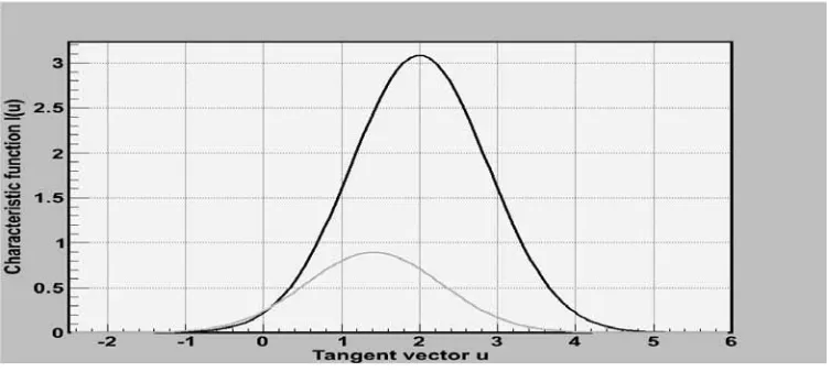
Figure 1 Plot of the characteristic function I(u) versus the tangent vector u.

The Blue color shows the behavior of the characteristic function with the presence of an external field, the Black color is for the characteristic function without the field, and the Red color is the characteristic function in an external field but opposite in direction with respect to the tangent vector.

Figure 2 Plot of the characteristic function I(u) versus the tangent vector u

The Blue color shows the behavior of the characteristic function of the WLC with very very small bending and the Green color is the characteristic function of the WLC with observable bending.

(8)

CONCLUSION AND RECOMMENDATION

The results tell us that introducing an external field to the wormlike chain particularly increases the peak of the probability distribution. When the direction from the external field vector is taken to be opposite in direction of the tangent vector, the peak of the probability distribution is even smaller than when the external field is set to zero. Also, the probability of a certain range of u is higher when we assume that there is more bending in the WLC than the probability when we neglect the bending of the WLC.

We can now also conclude that the application of white noise analysis can be extended to the wormlike chain model. However, we note that the _cosθ, which is due to the operation of the dot product between the tangent vector and the field vector, is approximated to small angle so that _cosθ_{� � �}θ�

�. This approximation implies that we are considering a short wormlike chain polymer. Thus, it is still desirable that this angle is not assumed to be small. In this case, one can consider both short and long wormlike chain polymers.

LITERATURE CITED

Bernido C. C. and M. V. Carpio-Bernido. (2003).White Noise Path Integrals: Applications in Polymer Entanglement, in A Garden of Quanta - Essays in Honor of Hiroshi Ezawa, eds. J. Arafune et. Al (World Scientific, Singapore). 115-129.

Feynman R. P. and A. R. Hibbs. (1965). Quantum Mechanics and Path Integrals. McGraw, New York.

Grosche C. and F. Steiner. (1998). Handbook of Feynman Integrals. Berlin: Springer.

Marko J. and E. Siggia. (1995). Stretching DNA, Macromolecules 28, 8759-8770.

Streit L. and T. Hida. (1983). Generalized Brownian functionals and the Feynman integral, Stoch. Proc. Appl. 16. 55-69.

Taute K.M., F. Pamaloni, E. Frey and E. L. Florin. (2008). Microtubule Dynamics Depart from the wormlike chain model, Phys. Review Letters 100, 028102.

Yamakawa H. (1976). Statistical Mechanics of Wormlike Chains, Pure and Appl. Chem., 46. 135-141.

CONCLUSION AND RECCOMMENDATION

The results tell us that introducing an external field to the wormlike chain particularly increases the peak of the probability distribution. When the direction from the external field vector is taken to be opposite in direction of the tangent vector, the peak of the probability distribution is even smaller than when the external field is set to zero. Also, the probability of a certain range of u is higher when we assume that there is more bending in the WLC than the probability when we neglect the bending of the WLC.

We can now also conclude that the application of white noise analysis can be extended to the wormlike chain model. However, we note that the _cosθ, which is due to the operation of the dot product between the tangent vector and the field vector, is approximated to small angle so that _cosθ_{� � �}θ�

�. This approximation implies that we are considering a short wormlike chain polymer. Thus, it is still desirable that this angle is not assumed to be small. In this case, one can consider both short and long wormlike chain polymers.

LITERATURE CITED

Bernido, CC & MV Carpio-Bernido. (2003).White Noise Path Integrals: Applications in Polymer Entanglement, in A Garden of Quanta - Essays in Honor of Hiroshi Ezawa, eds. J. Arafune et. Al (World Scientific, Singapore). 115-129.

Feynman, RP & AR Hibbs. (1965). Quantum Mechanics and Path Integrals.

McGraw, New York.

Grosche, C & F Steiner. (1998). Handbook of Feynman Integrals. Berlin: Springer.

Marko, J & E Siggia. (1995). Stretching DNA. Macromolecules, 28:8759-8770.

Streit, L & T Hida. (1983). Generalized Brownian functionals and the Feynman integral. Stoch. Proc. Appl., 16:55-69.

Taute, KM, F Pamaloni, E Frey & EL Florin. (2008). Microtubule Dynamics Depart from the wormlike chain model. Phys. Review Letters 100, 028102.

(9)

Some Applications of the

Distribution of the Maximum on Independent

Normal Random Variables

Roberto N. Padua Liceo de Cagayan Date Submitted: February 20, 2011

Date Revised: June 24, 2011

ABSTRACT

The paper deals with the distribution of the maximum of n independent normal random variables and some of its applications in the electricity power industry in the area of peak load estimation and in genetic selection for animal breeding. For small n, the difficulty in finding the value of multiple integrals involved in the distribution function of the maximum order statistics (and hence, in the computation of its expected value) is recognized. The paper provides for simple approximations to the mean of the largest order statistics both in the iid and non-identically distributed cases. Large sample asymptotic results for extreme values of normal random variables are often used in reliability theory and of late, used in the analysis of extreme weather changes in relation to climate change. While the large sample results for the iid case have been treated in the past, we focused on the relatively unexplored non-identical but independent case. Results show that : (a) the simple approximations to the mean of the largest order statistic both for the iid and non-iid cases have good MSE properties, and (b) the large sample distribution for a non-identically distributed case still obeys the Type I Gumbel distribution with shifted parameters.

Keywords: largest order statistic, multivariate normal, error function, peak load, genetic selection, Rayleigh Distribution, Gumbel Distribution

INTRODUCTION

The hourly load demand for electricity as noted by an Electric Cooperative roughly follows a normal distribution so that if Xj represents the demand at hour j, then Xj ~ N(μj,σj2). We seek the probability that the peak demand occurs at hour t, that is, we want to evaluate:

(1) ...Pr(Xt>Y)

where Y=max{Xi},i≠t

Such a practical problem occurs almost daily in most industries in the country so that the need to develop analytic methods to tackle it is almost imperative. In the case that there are only two (2) potential peak hours, X1 and X2, then the Pr(X1>Y2) can be easily calculated. In fact, this is equivalent to

finding the probability, Pr(X1 – X2 > 0) which can be obtained from the

(10)

distribution N(μ1-μ2, σ12 +σ22) by a table look up or actual numerical integration.

When there are n competing hours, then one must resolve Equation (1) which is the focus of the present paper.

The problem of finding the distribution of Y is, by itself, nothing new. In fact, the classical approach would be to consider:

...Pr(Y≤y) = Pr(X1≤y‚ X2≤y‚ … xn≤y) = πPr(Xi≤y) = πφi(y) (2)

where Φi(.) is the cumulative distribution function of a normal distribution with

mean μi and variance σi2. The probability problem given by (1) reduces to:

...Pr(Y≤y)=1-Pr(Xt≤Y|Y)πPr(Y≤Y) (3)

Equation (3) demands a large amount of integration and we shall not approach the problem this way.

A related problem arises out of this basic problem of determining the probability distribution of the maximum of n independent normal random variables. Consider the daily peak loads noted Y1,Y2,...,Yn for a period n. The

distribution of each Yi is given by (2) and will be more explicitly stated in the

body of this paper. We wish to know the joint distribution of these peak loads f(Y1,Y2,..,Yn). Knowledge of the joint distribution f(.) allows us to ask relevant

questions such as, “What is the probability that the daily peak loads do not exceed a capacity limit L?” That is, we seek answer to the probability question:

...Pr(Y1≤L,Y2≤L,...Yn≤L)? (4)

With the passage of the Electricity Power Industry Reform Act (1998), the issues of generation capacity and demand requirements, average and peak load requirements and others had been highlighted because of the unbundling of the electricity charges passed on to the consumers. For instance, distribution utilities have to contend with the issue of determining how much electricity to procure from power generation companies considering both the average demand and the peak load demand in their service areas. A miscalculation on the part of the distribution utilities could mean millions in terms of losses.

Hill (2010) considered a similar problem in relation to the calculation of the probability that a runner wins in an n-player running match. Specifically, he obtained the probability distribution of the minimum of n independent normal random variables. He found that the probability distribution of Y, the minimum of n independent normal random variables obeys a multivariate

normal distribution with mean vector μ and covariance matrix S where:

(11)

... μ = (μ1, μ2,...,μn)’ and S = diag(σi2) is a diagonal matrix

with σi2 on the ith diagonal and zeroes elsewhere. (5)

or

...�� _{√�� √��}� _�� (6)

The application of Hill’s (2010) results in more practical areas such as the power industry sector is obvious. One might be interested in the downtime power load (instead of the peak power load) for purposes of planning and forecasting of a distribution utility’s daily demand requirements.

Finally, a related problem that might be of interest is the probability

distribution of the maximum of the maxima of random variables. Let S1 = {x11,

x12,...,x1n}, S2 = {x21,x22,...,x2n},..., Sp={x1p,x2p,...,xpn} be subsets of independent random variables of equal length n. Let :

… �� (7)

…� � �� … � �

We are interested in computing the probability that Pr(T > a). As a practical application of this problem, consider the hourly demand for electricity on a daily basis over a one-month period. The subsets Si consists of the hourly

demand records (n = 24). The maxima Yi represents the peak demand for the

ith day. The random variable T represents the peak of the peak demands over a one month period. Knowing the probability distribution of the Y’s can be used to calculate the desired probability distribution of T.

Mathematical Derivation of the Distribution of the Maxima of n Normal Random Variables

We are interested in evaluating Pr(X0 > Y) where Y = max { Xj } j = 1,2,..,n with the same assumptions as Hill’s(2010) paper. Following his derivation, we first obtain the probability distribution of Y:

Pr�� (8)

_{� ��}�

��

��√��)

= _� �

√�� _��_… ��

��√�

��

� √��

��_��

��√�

�� dx1...dxn

= � ��

��√��

��_��_��_{��}

��

(12)

Hence, the probability distribution of the maximum of n independent normal random variables is precisely a multivariate normal distribution where:

� � �� .

Let us write down the density function of X0 as:

g(x) = � �_{� √��}��

�

��

We seek the probability _��_�_{� ��.}

��

� ��

= _{� ��}_�� _�_{��}_�_�� and the outer integral is from (-_{�� }. (9)

However, the integral is precisely the integral of an (n+1)-variate normal distribution or the n-variate normal distribution before plus one additional variable. That is,

h(t) = �

�� √��

��_��_��_{��}

(10)

where S is an (n+1) x (n+1) strictly diagonal positive definite matrix whose diagonal elements are σi2 , i = 0,1,...,n and μ = (μ0, μ1,..., μn). The computation of the integral , however, is not a trivial task and we shall return to this issue later when we perform our simulation exercises.

Application 1: Given the hourly data for electricity demand in a given locality, we can ask the question of finding the probability that the peak demand is less than 50MW. If X1,X2,..,X24 are the hourly electricity demands, and Y = max {Xi}, then we can compute P(Y ≤ 50) using Equation (8). Of course, we need the hourly data (24-hour data) over at least one month to establish the distribution of the X’s.

(13)

The animal with score X(n) is to be selected. If X1; . . . ;Xn are independent with mean μ, then the common mean of the observations of offsprings of the selected animal with score X(n) is E(X(n)), and therefore the expected gain in one generation is E(X(n)) - μ. The assumption of independence will be violated if the pigs come from the same stock and so we make sure that the animals to be observed come from different stocks. If Y = max{Xi} we can ask the same probability question as before.

Independent and Identically (IID) Normal Random Variables Case

Often, our interest rests mainly on the mean of the maximum of n random variables. Even in the case where the random variables are normally distributed, the numerical integration required to determine the expected value of the maximum is tedious. It is possible to develop heuristic approximations to the expected value of the maximum of n iid normal random variables.

Let X(n) = max {Xi}. Clearly X(n) > E(Xi) = μ for all i. Suppose that:

X(n) = μ + ε where ε ~ F(ε) , and (11)

F(ε) = 1 – exp(-��

��) , 0 < ε < ∞

The distribution F(.) is called a Rayleigh Distribution used in extreme value analysis and is a special case of the Weibull distribution with α = _√2 b and β = 2.. The Rayleigh distribution has been used to model the distance covered per unit time of a particle whose (x,y) coordinates are each independent standard normal random variables. Model 11 says that the maximum order statistic X(n) exceeds the mean of the component normal random variables by a random amount ε whose expected value is :

E(ε) = _√2 b Γ(1 + ½) (12)

The expected value of X(n) can be obtained from (11):

E(X(n)) = μ + E(ε). (13)

In other words, if we can model the extreme value statistic X(n) as a sum of the common mean plus a Rayleigh distributed random error, then it is possible to estimate its mean as well by (13).

(14)

Procedurally, if x1,x2,..,xn are iid N(μ,σ2) are random samples, then we

first take the maximum likelihood estimators of μ and σ2_{corrected for bias:}

� � = �

�∑xi (14)

s2₌ �

��∑ (xi – � �)2

Put εi = �xi – � �� for i = 1, 2, ...,n, which we now assume obeys the

Rayleigh distribution with mean equal to (13). The maximum likelihood estimator of the parameter b of the Rayleigh distribution is given by:

b = �_�� ∑ �� _��

� (15)

Our estimate for E(X(n)) = μ(n) is thus:

�� = � � + 2√��_�� ∑ �� = � � + √2��_��∑ �� ≈ � � + 2.51 sd(x) (16)

Or heuristically, �� = � � + 3 sd(x) which is intuitively appealing. We verify this error model by using simulation in the next section.

Independent but not Identically Distributed Normal Random Variables

The situation when the random variables Xi are not identically distributed

but independent normal random variables with μi = E(Xi) and σi2 = var(Xi) is

more complicated but also more useful in practice. In the succeeding discussions, we agree on the following notation:

�� = �

� ∑ �� = mean of the means

μ(n) = max { μ1, μ2, ..., μn} = maximum of the means

X(n) = max { X1,X2,...,Xn} = maximum order statistic

Dn = μ(n) - ��

We create a data model similar to (11). We start with the obvious inequality: μ(n) - �� ≥ 0 with equality only if μi = μ for all i. (17) Procedurally, if x1,x2,..,xn are iid N(μ,σ2_{) are random samples, then we}

first take the maximum likelihood estimators of μ and σ2_{corrected for bias:}

� � = �

�∑xi (14)

s2₌ �

��∑ (xi – � �)2

Put εi = �xi – � �� for i = 1, 2, ...,n, which we now assume obeys the Rayleigh distribution with mean equal to (13). The maximum likelihood estimator of the parameter b of the Rayleigh distribution is given by:

b = �_�� ∑ �� _��

� (15)

Our estimate for E(X(n)) = μ(n) is thus:

�� = � � + 2√��_�� ∑ �� = � � + √2��_��∑ �� ≈ � � + 2.51 sd(x) (16)

Or heuristically, �� = � � + 3 sd(x) which is intuitively appealing. We

verify this error model by using simulation in the next section.

Independent but not Identically Distributed Normal Random Variables

The situation when the random variables Xi are not identically distributed

but independent normal random variables with μi = E(Xi) and σi2_{= var(Xi) is}

more complicated but also more useful in practice. In the succeeding discussions, we agree on the following notation:

�� = �

� ∑ �� = mean of the means

μ(n) = max { μ1, μ2, ..., μn} = maximum of the means X(n) = max { X1,X2,...,Xn} = maximum order statistic Dn = μ(n) - ��

We create a data model similar to (11). We start with the obvious inequality:

μ(n) - �� ≥ 0 with equality only if μi = μ for all i. (17)

To see this, consider:

μ(n) = �

�∑ �� > ��

�∑ �� = �� since μ(n) > μi for all i. (18) It follows that Dn ≥ 0.

We now claim that :

X(n) = �� + εi where εi = �xi - ��, i = 1,2,..,n. (19)

and : εi ~ F(ε) is a Rayleigh distribution function.

In practice, the underlying means are unknown and so we replace (19) by its sample counterpart:

X(n) = _��+ �xi - _�_��. (20)

The second term on the right is assumed to obey a Rayleigh distribution with the mean given by Equation (12). However, the MLE of b is now:

�� = �_�� ∑ �� . (21)

Equation (21) is no longer approximately equal to _√2 sd(x). We can argue heuristically to obtain a sense of the magnitude of (21) in relation to the case when the xi’s are properly centered around their means.

Let Y = (x1-μ1)2_{+ (x2 – μ2)}2_{+...+ (xn – μn)}2_{, and Z =(x1-μ(n))}2_{+ (x2 – μ(n))}2 +...+ (xn – μ(n))2_{. If we take expectations:}

E(Y) = σ2_{+ σ}2_{+ ... + σ}2_{= nσ}2_, ₍₂₂₎

assuming equal variances. Next consider one term of the quantity Z:

E(xi – μ(n) )2_{= E(xi – μi + μi – μ(n) )}2_{= E(xi-μi)}2 ₍₂₃₎ + 2E(xi – μi)(μi – μ(n)) + E(μi – μ(n))2

= σ2_{+ 0 + θ1}2_{, since the second term above is zero} and θ12_{= (μi – μ(n))}2

It follows that E(Y) = nσ2_{≤ E(Z) = nσ}2₊_{∑ �} ��

� . Equation (21) is greater than Equation (15), and so we expect a greater additive factor to the expected value of the means than in the IID case. In fact, the inequality provides us an insight on the magnitude of the difference since:

(15)

μ(n) = �

�∑ �� > ��

We now claim that :

X(n) = �� + εi where εi = �xi - �_��, i = 1,2,..,n. (19)

X(n) = ��+ �xi - �_��.

(20)

�� = �_�� ∑ �� . (21)

Let Y = (x1-μ1)2 + (x2 – μ2)2 +...+ (xn – μn)2, and Z =(x1-μ(n))2 + (x2 – μ(n))2

+...+ (xn – μ(n))2. If we take expectations:

E(Y) = σ2_{+ σ}2_{+ ... + σ}2_{= nσ}2_, ₍₂₂₎

E(xi – μ(n) )2 = E(xi – μi + μi – μ(n) )2 = E(xi-μi)2 (23)

+ 2E(xi – μi)(μi – μ(n)) + E(μi – μ(n))2

= σ2_{+ 0 + θ}₁2_{, since the second term above is zero}

and θ12 = (μi – μ(n))2

It follows that E(Y) = nσ2_{≤ E(Z) = nσ}2₊_{∑ �}

��

E(Z) – E(Y) = ∑ �� . (24)

Padua: Some Applications of the Distribution of the Maximum

μ(n) = �

�∑ �� > ��

�∑ �� = �� since μ(n) > μi for all i. (18) It follows that Dn≥ 0.

We now claim that :

X(n) = �� + εi where εi = �xi - �_��, i = 1,2,..,n. (19)

X(n) = ��+ �xi - �_��.

(20)

�� = �_�� ∑ �� . (21)

Let Y = (x1-μ1)2 + (x2 – μ2)2 +...+ (xn – μn)2, and Z =(x1-μ(n))2 + (x2 – μ(n))2

+...+ (xn – μ(n))2. If we take expectations:

E(Y) = σ2₊_σ2_{+ ... +}_σ2_{= n}_σ2_, ₍₂₂₎

E(xi – μ(n) )2 = E(xi – μi + μi – μ(n) )2 = E(xi-μi)2 (23)

+ 2E(xi – μi)(μi – μ(n)) + E(μi – μ(n))2

= σ2_{+ 0 +}_θ₁2_{, since the second term above is zero}

and θ12 = (μi – μ(n))2

It follows that E(Y) = nσ2_≤_{E(Z) = n}_σ2₊_{∑ �}

��

E(Z) – E(Y) = ∑ �� . (24)

μ(n) = �

�∑ �� > ��

We now claim that :

X(n) = �� + εi where εi = �xi - ��, i = 1,2,..,n. (19)

X(n) = _��+ �xi - _�_��. (20)

�� = �_�� ∑ �� . (21)

Let Y = (x1-μ1)2_{+ (x2 – μ2)}2_{+...+ (xn – μn)}2_{, and Z =(x1-μ(n))}2_{+ (x2 – μ(n))}2 +...+ (xn – μ(n))2_{. If we take expectations:}

E(Y) = σ2_{+ σ}2_{+ ... + σ}2_{= nσ}2_, ₍₂₂₎

E(xi – μ(n) )2_{= E(xi – μi + μi – μ(n) )}2_{= E(xi-μi)}2 ₍₂₃₎ + 2E(xi – μi)(μi – μ(n)) + E(μi – μ(n))2

= σ2_{+ 0 + θ1}2_{, since the second term above is zero} and θ12_{= (μi – μ(n))}2

It follows that E(Y) = nσ2_{≤ E(Z) = nσ}2₊_{∑ �} ��

(16)

There is a rough approximation on the value of E(X(n)) provided by Hamza(2008) and we borrow his theorem below:

Theorem (Hamza). Let X1,X2,..,Xn be independent random variables with Mi = E(Xi), then:

ܯഥ≤ E(X(n)) ≤ܯഥ + ௡ିଵ

௡ M(n).

where:

_ܯഥ = average of the Mi’s

M(n) = max{Mi}.

In relation to the present problem, it may often be more useful for the electric distribution utility to have an idea of the magnitude of the peak demand (on the average). Thus, Hamza’(s) (2008) theorem will be most useful in providing such information. Similarly, in the genetic selection problem of application 2, we can assume that the means differ across the animals and that we chose the maximum observed Xi as the animal to be used for breeding. Then, again , Hamza’s(2008) results will apply. Note that the Theorem does not require that the random variables be normal. It applies to all independent random variables, and so, is quite general.

Meanwhile for sufficiently large n, we can consider some asymptotic results to simplify the calculations.

Asymptotic Results for the IID Case

We wish to show that for large n, the asymptotic distribution of the largest

order statistic X(n) is a Gumbel Type I distribution. The Fisher–Tippet–

Gnedenko theorem (also the Fisher–Tippet theorem or the extreme value theorem) is a general result regarding asymptotic distribution of extreme order statistics. The maximum of a sample of iid random variables after proper renormalization converges in distribution to one of three possible distributions, the Gumbel distribution, the Fréchet distribution, or the Weibull distribution. Credit for the extreme value theorem (or convergence to types theorem) is given to Gnedenko (1948); previous versions were stated by Fisher and Tippett in 1928 and Fréchet in 1927. The role of the extremal types theorem for maxima is similar to that of the central limit theorem for averages.

Let Y = max {Xi} of a sequence of independent and identically distributed

standard normal random variables Xi. Let Φ(x) denote the cumulative

distribution function of a standard normal random variable x. The cumulative distribution function of the maximum order statistic Y is:

Fn(y) = [Φ(y)]n , -∞ < y < ∞ as before (25)

There is a rough approximation on the value of E(X(n)) provided by Hamza(2008) and we borrow his theorem below:

Theorem (Hamza). Let X1,X2,..,Xn be independent random variables with Mi = E(Xi), then:

ܯഥ≤ E(X(n)) ≤ܯഥ + ௡ିଵ

௡ M(n). where:

_ܯഥ = average of the Mi’s M(n) = max{Mi}.

In relation to the present problem, it may often be more useful for the electric distribution utility to have an idea of the magnitude of the peak demand (on the average). Thus, Hamza’(s) (2008) theorem will be most useful in providing such information. Similarly, in the genetic selection problem of application 2, we can assume that the means differ across the animals and that we chose the maximum observed Xi as the animal to be used for breeding. Then, again , Hamza’s(2008) results will apply. Note that the Theorem does not require that the random variables be normal. It applies to all independent random variables, and so, is quite general.

Meanwhile for sufficiently large n, we can consider some asymptotic results to simplify the calculations.

Asymptotic Results for the IID Case

We wish to show that for large n, the asymptotic distribution of the largest order statistic X(n) is a Gumbel Type I distribution. The Fisher–Tippet– Gnedenko theorem (also the Fisher–Tippet theorem or the extreme value theorem) is a general result regarding asymptotic distribution of extreme order statistics. The maximum of a sample of iid random variables after proper renormalization converges in distribution to one of three possible distributions, the Gumbel distribution, the Fréchet distribution, or the Weibull distribution. Credit for the extreme value theorem (or convergence to types theorem) is given to Gnedenko (1948); previous versions were stated by Fisher and Tippett in 1928 and Fréchet in 1927. The role of the extremal types theorem for maxima is similar to that of the central limit theorem for averages.

Let Y = max {Xi} of a sequence of independent and identically distributed standard normal random variables Xi. Let Φ(x) denote the cumulative distribution function of a standard normal random variable x. The cumulative distribution function of the maximum order statistic Y is:

(17)

Clearly, lim Fn(y) = 1 or 0 depending on whether Φ(y) = 1 or 0 as n →∞. In

order to obtain a non-degenerate limiting distribution, it is necessary to transform Y by applying a linear transformation with coefficients which depend on the sample size n but not on y. This process is similar to the standardization

process in statistics. Let Yn’ = anY + bn where an and bn are coefficients depending

on n but not on y. Suppose first that the limiting distribution G(y) exists. That is:

lim Fn(y) = G(y) exists for properly transformed Y.

If we increase the sample size to nN where N > 0, then the largest of the nN

values X1,X2,...,XnN is also equal to the largest of the values Xj-1(n+1), Xj-1(n+2),...,Xjn, for

j=1,2,...,N. It follows that the limiting distribution G(.) obeys:

[G(y)]N = G(a_Ny + b_N) (26)

Equation (26) is called the stability postulate and was first discovered by

Frechet (1927). Now, take aN = 1. Equation (26) now becomes:

[G(y)]N = G(y + b_N) (27)

We iterate Equation (27) for larger samples NM:

[G(y)]NM = G((x + b_NM) = G(y + b_N)M = G(y + bN + bM) (28)

We infer that : bNM = bN + bM . This equation tells that bN must be some type

of logarithmic function. In particular, bN = σ log N where σ is a constant. We

plug this value into Equation (27) to get:

[G(y)]N = G(y + σ log N ) (29)

Take the logarithm of both sides of (29) to get : N{- log G(y)} = - log G(y + σN) where the negative sign emerges from the fact that G(y) ≤ 1. We take the logarithm once again (sometimes called the law of iterated logarithms):

log N + log {- log G(y)} = log{- log G(y + σN)} (30)

Let h(y) = log {- log G(y)}. Equation (30) becomes:

log N + h(y) = h(σ(௬

ఙ + log N) or h(y ) = h(σ(

௬

ఙ + log N) – log N. (31)

(18)

Put σ(௬

ఙ + log N) = 0 (or find h(0) on the right hand side. This means that ௬

ఙ = - log N. Substituting back to Equation (31), we obtain:

h(y) = h(0) - ௬

ఙ, , since h(y) decreases as y increases. (32)

Thus, -logG(y) = exp(h(y)) = exp (h(0) - ௬

ఙ) = exp( - (

௬ିఙ௛ሺ଴ሻ

ఙ ). Put μ = σh(0)

and we have:

– log G(y) = exp (-(௬ିఓሻ

ఙ ). (33)

The last step is easy to see:

G(y) = exp (-exp (-(௬ିఓሻ

ఙ )) or G(y) = exp (-exp (-( ௬ିఈሻ

ఉ )). (34)

The asymptotic mean and variance of Y can now be obtained from G(y). It is an easy exercise to find the moments of this distribution:

The mean, variance, skewness, and kurtosis are

where is the Euler-Mascheroni constant and is Apéry's constant.

Asymptotic Results for the Independent but not Identically Distributed Case (INID)

Let X1,X2,...,Xn be independent normal random variables with means E(Xi) = μi and variances given by var(Xi) = σi2. As before, we let Y = max{Xi}. The distribution of Y is given by:

Fn*(y) = π[Fi(y)], i = 1 2,...,n (35)

(19)

without bound. In practice, it is the second interpretation that appears to be reasonable and implementable. Hence, our asymptotic analysis will follow the second interpretation.

To this end, let:

�� = �

� ∑ �� = arithmetic average of the means which is non-stochastic,

�� = �

� ∑ �� = arithmetic average of the variances, also non-stochastic

� � = �

√� �∑ �� = the square root of the arithmetic average of the

variances.

We consider:

Fn*(��

�� ) = π[Fi( ��

�� )], i = 1 2,...,n.

If samples of size M were obtained from each d.f., then:

Fn*(��

�� ) = π[Fi( ��

�� )]M, i = 1 2,...,n., M = 1,2,3,...→∞ (36)

Assume , as before , that the limiting distribution of (36) exists and is G(.):

π[Fi(��

�� )]M → G( ��

�� ) as M →∞. (37)

Applying the same stability postulate as before, we have:

G(��

�� M = G( ��

�� + bM) (38)

For which we conclude that bM = θ log M. Hence:

log M + log (-log(G(��

�� ) ) = log(-log(G( ��

�� + θ log M )). (39)

Equation (39) implies that if h(��

�� ) = log (-log(G( ��

�� ) ), then:

h(��

�� ) = h(0) - ��

�� = -( ��

�� - ��

�� h(0)) (40)

without bound. In practice, it is the second interpretation that appears to be reasonable and implementable. Hence, our asymptotic analysis will follow the second interpretation.

To this end, let:

�� = �

� ∑ �� = arithmetic average of the means which is non-stochastic,

��

�� = �

� ∑ �� = arithmetic average of the variances, also non-stochastic

� � = �

√� �∑ �� = the square root of the arithmetic average of the

variances.

We consider:

Fn*(��

�� ) = π[Fi( ��

�� )], i = 1 2,...,n.

If samples of size M were obtained from each d.f., then:

Fn*(��

�� ) = π[Fi( ��

�� )]M, i = 1 2,...,n., M = 1,2,3,...→∞ (36)

Assume , as before , that the limiting distribution of (36) exists and is G(.):

π[Fi(��

�� )]M → G( ��

�� ) as M →∞. (37)

Applying the same stability postulate as before, we have:

G(��

�� M = G(

��

�� + bM) (38)

For which we conclude that bM = θ log M. Hence:

log M + log (-log(G(��

�� ) ) = log(-log(G(

��

�� + θ log M )). (39)

Equation (39) implies that if h(��

�� ) = log (-log(G(

��

�� ) ), then:

h(��

�� ) = h(0) -

��

�� = -(

�� -

��

(20)

It follows that:

G(yሻ = exp (-exp(-ሺ௬ିఓഥ Ȃఙ_ఙ_{ഥ ఏ}ഥ ௛ሺ଴ሻሻ) (41)

which we recognize as a Type I Gumbel distribution with α = _ߤ_ഥ + _ߪ_ഥh(0) and β

= ߪഥߠ. Here h(0)= log(-log (G(0)).

LITERATURE CITED

Arellano-Valle, R.B., Genton, M.G. (2005). On fundamental skew distributions. J. Multivariate Anal. 96, 93–116.

Arellano-Valle, R.B., Genton, M.G. (2007). On the exact distribution of linear combinations of order statistics from dependent randomvariables. J. Multivariate Anal. in press.

Arellano-Valle, R.B., Branco, M.D., Genton, M.G. (2006). A unified view on skewed distributions arising from selections. Canad. J.Statist. 34, 581– 601.

Crocetta, C., Loperfido, N. (2005). The exact sampling distribution of L-statistics. Metron 63, 1–11.

David, H.A. (1981). Order Statistics. Wiley, New York.

Fang, K.-T., Kotz, S., Ng, K.-W. (1990). Symmetric multivariate and related distributions. Monographs on Statistics and AppliedProbability, vol. 36. Chapman & Hall, Ltd., London.

Genton, M.G. (2004). Skew-Elliptical Distributions and Their Applications: A Journey Beyond Normality. Edited volume, Chapman & Hall/CRC Press, London, Boca Raton, FL.

Genz, A. (1992). Numerical computation of multivariate Normal probabilities. J. Comput. Graph Statist. 1, 141–149.

Genz, A., Bretz, F. (2002). Methods for the computation of multivariate t-probabilities. J. Comput. Graph. Statist. 11, 950–971.

Ghosh, M. (1972). Asymptotic properties of linear functions of order statistics for m-dependent random variables. Calcutta Statist. Assoc.Bull. 21, 181–192.

It follows that:

LITERATURE CITED

Abdelkader, Y. (2005). Computing the moments of order statistics from

nonidentically distributed Erlang variables. Statistical Papers,

45(4):563-570.

Al–Shboul, QM & A Khan. (1989). Moments of order statistic from doubly

truncated log-logistic distribution. Pakistan J. Statist ., 5(3B):209-307.

Arellano-Valle, RB & MG Genton. (2005). On fundamental skew distributions. J. Multivariate Anal., 96:93–116.

Arellano-Valle, RB & MG Genton. (2007). On the exact distribution of linear

combinations of order statistics from dependent randomvariables. J. Multivariate Anal. in press.

Arellano-Valle, RB, MD Branco & MG Genton. (2006). A unified view on

skewed distributions arising from selections. Canad. J.Statist. 34:581–

601.

Ashour, SK & M El–Wakeel. (1993). Bayesian prediction of the jth order

statistics with Burr distribution and random sample size. Microelectron

Reliab., 33(8):1179–1188. J. Math. & Stat., 2 (3): 432-438, 2006 438.

Austin, JA Jr. (1973). Control Chart Constants for largest and Smallest in a Sampling from a Normal Distribution Using the Generalized Burr

Distribution. Technometrics, 15(4):130- 933.

Balakrishnan, N & K Balasubramanian. (1995). Order statistics from

non-identically Power function random variables. Commun. Statist.-Theory

Meth., 24(6):1443-1454.

Balakrishnan, N. (1994a). Order statistics from non-identically exponentically

random variables and some applications. Comput. Statist. Data- Anal.

18(2):203-225.

It follows that:

LITERATURE CITED

Arellano-Valle, R.B., Genton, M.G. (2005). On fundamental skew

distributions. J. Multivariate Anal. 96, 93–116.

Arellano-Valle, R.B., Genton, M.G. (2007). On the exact distribution of linear

Arellano-Valle, R.B., Branco, M.D., Genton, M.G. (2006). A unified view on

skewed distributions arising from selections. Canad. J.Statist. 34, 581– 601.

Crocetta, C., Loperfido, N. (2005). The exact sampling distribution of

L-statistics. Metron 63, 1–11.

David, H.A. (1981). Order Statistics. Wiley, New York.

Fang, K.-T., Kotz, S., Ng, K.-W. (1990). Symmetric multivariate and related

distributions. Monographs on Statistics and AppliedProbability, vol. 36. Chapman & Hall, Ltd., London.

Genton, M.G. (2004). Skew-Elliptical Distributions and Their Applications: A

Journey Beyond Normality. Edited volume, Chapman & Hall/CRC Press, London, Boca Raton, FL.

Genz, A. (1992). Numerical computation of multivariate Normal probabilities.

J. Comput. Graph Statist. 1, 141–149.

Genz, A., Bretz, F. (2002). Methods for the computation of multivariate

t-probabilities. J. Comput. Graph. Statist. 11, 950–971.

Ghosh, M. (1972). Asymptotic properties of linear functions of order statistics

(21)

Balakrishnan, N. (1994b). On order statistics from non-identical right-truncated exponential random variables and some applications. Commun. Statist. – Theory Meth. 23:3373- 3393.

Bapat, R & M Beg. (1989). Order Statistics from non-identically distributed variables and permanents. Sankh~Ya, A, 51:79-93.

Barakat, H & Y Abdelkader. (2000). Computing the moments of order statistics from nonidentically distributed Weibull variables. J. Comp. Appl. Math. 117(1): 85-90.

Barakat, H & Y Abdelkader. (2004). Computing the Moments of order statistics from nonidentical random variables. Statistics Methods & Applications, 13:15-26.

Burr, IW & P Cislak. (1968). On general system of distribution I. Its curve shape characteristics II. The Sample Median. Jour. Amer. Statist. Assn., 62:627–635.

Burr, IW. (1942). Cumulative frequency functions. Annals of mathematical statistics, 13:215 232.

Burr, IW. (1967). A Useful Approximation to the Normal Distribution Function, with Application to Simmulation. Technometrics, 9(4):647-651.

Burr, IW. (1968). On a General system of Distributions. III the Sample Range. Journal American Statist. Assn ., 62:637-643.

Childs, A & N Balakrishnan. (1995a). Generalized recurrence relations for moments of order statistics from non-identical doublytruncated random variables. Preprint.

Childs, A & N Balakrishnan. (1995b). Relations for single moments of order statistics from non-identical logistic random variables and assessment of the effect of multiple outliers on the bias of linear estimators of location and scale. Preprint.

Childs, A & N Balarishnan. (1998). Generalized recurrence relations for moments of order statistics from non-identical Pareto and truncated Pareto random variables with applications to robustness. In: Balakrishnan N, Rao RC (eds) Handbook of statistics, 16, North-Holland, Amsterdam: 403-438.

It follows that:

LITERATURE CITED

Arellano-Valle, R.B., Genton, M.G. (2005). On fundamental skew

distributions. J. Multivariate Anal. 96, 93–116.

Arellano-Valle, R.B., Genton, M.G. (2007). On the exact distribution of linear

Arellano-Valle, R.B., Branco, M.D., Genton, M.G. (2006). A unified view on

skewed distributions arising from selections. Canad. J.Statist. 34, 581– 601.

Crocetta, C., Loperfido, N. (2005). The exact sampling distribution of

L-statistics. Metron 63, 1–11.

David, H.A. (1981). Order Statistics. Wiley, New York.

Fang, K.-T., Kotz, S., Ng, K.-W. (1990). Symmetric multivariate and related

distributions. Monographs on Statistics and AppliedProbability, vol. 36. Chapman & Hall, Ltd., London.

Genton, M.G. (2004). Skew-Elliptical Distributions and Their Applications: A

Journey Beyond Normality. Edited volume, Chapman & Hall/CRC Press, London, Boca Raton, FL.

Genz, A. (1992). Numerical computation of multivariate Normal probabilities.

J. Comput. Graph Statist. 1, 141–149.

Genz, A., Bretz, F. (2002). Methods for the computation of multivariate

t-probabilities. J. Comput. Graph. Statist. 11, 950–971.

Ghosh, M. (1972). Asymptotic properties of linear functions of order statistics

(22)

Coa, G & M West. (1977). Computing distributions of order Statistics. Common. Statist. – Theory meth., 26(3):755-764.

Crocetta, C & N Loperfido. (2005). The exact sampling distribution of L-statistics. Metron, 63:1–11.

David, HA. (1981). Order Statistics. Wiley, New York.

Evans, IG & A Ragab. (1983). Bayesian inferences given a type – 2 censored sample from a Burr distribution. Commun. Statist. th. Methods A,

12(1):1569–1580.

Fang, KT, S Kotz & KW Ng. (1990). Symmetric multivariate and related distributions. Monographs on Statistics and Applied Probability, vol. 36. Chapman & Hall, Ltd., London.

Galambos, J. (1987). The Asympototic Theory of Extreme Order Statistics, 2nd edn. Krieger, Malabar, Florida

Genton, MG. (2004). Skew-Elliptical Distributions and Their Applications: A Journey Beyond Normality. Edited volume, Chapman & Hall/CRC Press, London, Boca Raton, FL.

Genz, A & F Bretz. (2002). Methods for the computation of multivariate t-probabilities. J. Comput. Graph. Statist., 11:950–971.

Genz, A. (1992). Numerical computation of multivariate Normal probabilities.

J. Comput. Graph Statist., 1:141–149.

Ghosh, M. (1972). Asymptotic properties of linear functions of order statistics for m-dependent random variables. Calcutta Statist. Assoc.Bull.,

21:181–192.

Gupta, PL, RC Gupta & SJ Lvin. (1996). Analysis of failure time data by Burr distribution. Common. Statist Theory Meth., 25(9): 2013 – 2024.

Hill, WG. (1977). Order statistics of correlated variables and implications in genetic selection programmes. II. Response to selection.Biometrics 33, 703–712.

(23)

Lomax, KS. (1954). Business Failures: AnotherExample of the Analysis of Failure Data. J. American Statist Assoc., 847-852.

Minc, H. (1978). Permanents, Encyclopedia of Mathematics and its applications 6, Addison-Wesley, Reading, MA.

Minc, H. (1983). Theory of permanents (1978 - 1981). Linear and multilinear Algebra, 12: 227-263.

Minc, H. (1987). Theory of permanents (1982 - 1985). Linear and multilinear Algebra, 12: 227-263.

Nigm, AM & NY Abd Al–Wahab. (1996). Bayesian prediction with a random sample size for the Burr life distribution. Commun Statist – Theory Meth., 25(6):1289–1303.

Pandey, M & B Uddin. (1991). Estimation of reliability in Multi – Component stress – strength model following a Burr distribution. Microelectron. Reliab., 31(1):21–25.

Papdopoulos, AS. (1978). The Burr distribution as a failure model from a Bayesian approach. IEEE Trans. On Rel., 5:369–371.

Ragab, A & J Green. (1984). On Order Statistics From the Log-Logistic Distribution and Their Properties. Comm.in Statistics, A13:21.

Rawlings, JO. (1976). Order statistics for a special class of unequally correlated multinormal variates. Biometrics, 32:875–887.

Rodriguez, NR. (1977). A Guide to the Burr type XII distribution. Biometrika, 54(1):129–134.

Tadikamalla, PR & J Ramberg. (1975). An Approximate Method for Generating Gamma and Other Variates. J.Statist Comput. Simul., 3:375-382.

Tadikamalla, PR. (1977). An Approximation to the Moments and the Percentiles of Gamma Order Statistics . Sankya: The Indian Journal of Statistics, 39(B4):372-381.

Tadikamalla, PR. (1980). A Look at the Burr and Related Disatribution. Intl. Statistical Review, 48:337-344.

(24)

Wheeler, D. (1975). An Approximation for Simulation of Gamma Distributions. Statist. Comput. Simul., 3:225- 232.

Wingo, DR. (1993b). Maximum likelihood methods for fitting the Burr type XII distribution to multiply (Progressively) censored life test data. Metrika, 40:203–210.