Non-singular spherical harmonic expressions of geomagnetic vector and gradient tensor fields in the local north-oriented reference frame

www.geosci-model-dev.net/8/1979/2015/ doi:10.5194/gmd-8-1979-2015

© Author(s) 2015. CC Attribution 3.0 License.

Non-singular spherical harmonic expressions of geomagnetic vector

and gradient tensor fields in the local north-oriented reference frame

J. Du1,2,3, C. Chen1, V. Lesur2, and L. Wang1,3

1_{Hubei Subsurface Multi-scale Imaging Key Laboratory, Institute of Geophysics & Geomatics,} China University of Geosciences, Wuhan 430074, China

2_{Helmholtz Centre Potsdam, GFZ German Research Centre for Geosciences, Telegrafenberg 14473, Potsdam, Germany} 3_{State Key Laboratory of Geodesy and Earth’s Dynamics, Chinese Academy of Sciences, Wuhan 430077, China}

Correspondence to: J. Du ([email protected])

Received: 27 October 2014 – Published in Geosci. Model Dev. Discuss.: 05 December 2014 Revised: 23 May 2015 – Accepted: 15 June 2015 – Published: 07 July 2015

Abstract. General expressions of magnetic vector (MV) and magnetic gradient tensor (MGT) in terms of the first- and second-order derivatives of spherical harmonics at differ-ent degrees/orders are relatively complicated and singular at the poles. In this paper, we derived alternative non-singular expressions for the MV, the MGT and also the third-order partial derivatives of the magnetic potential field in the lo-cal north-oriented reference frame. Using our newly derived formulae, the magnetic potential, vector and gradient ten-sor fields and also the third-order partial derivatives of the magnetic potential field at an altitude of 300 km are calcu-lated based on a global lithospheric magnetic field model GRIMM_L120 (GFZ Reference Internal Magnetic Model, version 0.0) with spherical harmonic degrees 16–90. The cor-responding results at the poles are discussed and the validity of the derived formulas is verified using the Laplace equation of the magnetic potential field.

1 Introduction

Compared to the magnetic vector and scalar measurements, magnetic gradients lead to more robust models of the litho-spheric magnetic field. The ongoing Swarm mission of the European Space Agency (ESA) provides measurements not only of the vector and scalar data but also an estimate of their east–west gradients (e.g., Olsen et al., 2004, 2015; Friis-Christensen et al., 2006). Kotsiaros and Olsen (2012, 2014) proposed to recover the lithospheric magnetic field through magnetic space gradiometry in the same way that has been

done for modeling the gravitational potential field from the satellite gravity gradient tensor measurements by the Gravity field and steady-state Ocean Circulation Explorer (GOCE). Purucker (2005), Purucker et al. (2007), Sabaka et al. (2015) and Kotsiaros et al. (2015) also reported efforts to model the lithospheric magnetic field using magnetic gradient infor-mation from the satellite constellation. Their results showed that, by using gradient data, the modeled lithospheric mag-netic anomaly field has enhanced shorter wavelength content and a much higher quality compared to models built from vector field data. This is because the gradient data can re-move the highly time-dependent contributions of the mag-netosphere and ionosphere that are correlated between two side-by-side satellites.

gradient to interpret the satellite-altitude magnetic anomaly data. Therefore, both the magnetic field modeling and also the geological interpretations require the calculation for the partial derivatives of the magnetic field, possibly at the poles for specific systems of coordinates. Spherical harmonic anal-ysis, established originally by Gauss (1839), is generally used to model the global magnetic internal fields of Earth and other terrestrial planets (e.g., Maus et al., 2008; Langlais et al., 2010; Thébault et al., 2010; Finlay et al., 2010; Lesur et al., 2013; Sabaka et al., 2013; Olsen et al., 2014). Series of spherical harmonic functions themselves made of Schmidt semi-normalized associated Legendre functions (SSALFs) (e.g., Blakely, 1995; Langel and Hinze, 1998) are fitted by least squares to magnetic measurements, giving the spherical harmonic coefficients (i.e., the Gaussian coefficients) defin-ing the model. Kotsiaros and Olsen (2012, 2014) presented the MV (magnetic vector) and the MGT (magnetic gradi-ent tensor) using a spherical harmonic represgradi-entation and, of course, their expressions are singular as they approach the poles. Even if there are satellite data gaps around the poles, it is advisable to use non-singular spherical harmonic expres-sions for the MV and the MGT in case airborne or shipborne magnetic data are utilized (e.g., Golynsky et al., 2013; Maus, 2010). A rotation of the coordinate system is always possible to avoid the polar singularity, but this solution is very inef-fective for large data sets.

In this paper, following Petrovskaya and Vershkov (2006) and Eshagh (2008, 2009) for the gravitational gradient ten-sor in the local north-oriented, orbital reference and geocen-tric spherical frames, the non-singular expressions in terms of spherical harmonics for the MV, the MGT and the third-order derivatives of the magnetic potential field in the spe-cially defined local-north-oriented reference frame (LNORF) are presented. In the next section, the traditional expressions of the MV and the MGT are first stated, some necessary propositions are then proved and, lastly, new non-singular expressions are derived. In Sect. 3, the new formulae are tested using the global lithospheric magnetic field model GRIMM_L120 (GFZ Reference Internal Magnetic Model, version 0.0) (Lesur et al., 2013) and compared with the re-sults by traditional formulae. Finally, some conclusions are drawn and further applications are also discussed.

2 Methodology

In this section, the traditional expressions of MV and MGT are presented and their numerical problems are stated. Then, based on some necessary mathematical derivations, new ex-pressions are given.

2.1 Traditional expressions

The scalar potentialV of Earth’s magnetic field in a source-free region can be expanded in the truncated series of

spher-ical harmonics at the pointP (r,θ,ϕ) with the geocentric distancer, co-latitudeθand longitudeϕ(e.g., Backus et al., 1996):

V (r, θ, φ)=a

L X l=1

l X m=0

(a r)

l+1

g_lmcosmφ+hm_l sinmφPe_lm(cosθ ) , (1)

wherea=6371.2 km is the radius of Earth’s magnetic ref-erence sphere;Pe_lm(cosθ )(or Pe_lm for simplification) is the

SSALF of degreel and orderm;Lis the maximum spher-ical harmonic degree; andg_lm andhm_l are the geomagnetic harmonic coefficients describing Earth’s internal sources.

If considered in the LNORF{x, y, z}(e.g., Olsen et al., 2010), where thezaxis points downward in the geocentric radial direction, thexaxis points to the north, and theyaxis towards the east (that is, a right-handed system). At the poles, we define that thexaxis points to the meridian of 180◦_{E (or} 180◦W) at the North Pole and of 0◦at the South Pole, which will be discussed in Sect. 3. Therefore, the three components of the MV can be expressed as

Bx(r, θ, φ)= −1_r∂(−∂θ )V (r, θ, φ)

=

L P l=1

l P m=0

(a_r)l+2

gm_l cosmφ+hm_l sinmφ

h

d

dθPe_lm(cosθ ) i

,

(2a)

By(r, θ, φ)= −_rsin1_θ∂φ∂ V (r, θ, φ)

=

L P l=1

l P m=0

(a_r)l+2m

gm_l sinmφ−hm_l cosmφh_sin1_θPe_lm(cosθ ) i

,

(2b)

Bz(r, θ, φ)= −_∂(−∂r)V (r, θ, φ)

= −

L P l=1

l P m=0

(l+1) (a_r)l+2

gm_l cosmφ+hm_l sinmφPe_lm(cosθ ) .

(2c)

The MGT can be written as (e.g., Kotsiaros and Olsen, 2012)

∇B= 



Bxx Bxy Bxz

Byx Byy Byz

Bzx Bzy Bzz 

=





∂Bx/∂x ∂Bx/∂y ∂Bx/∂z

∂By/∂x ∂By/∂y ∂By/∂z

∂Bz/∂x ∂Bz/∂y ∂Bz/∂z 

, (3)

where nine elements are expressed respectively as

Bxx=1_a L P l=1

l P m=0

(a_r)l+3 g_lmcosmφ+hm_l sinmφ ×h−d2

dθ2Pe_lm(cosθ )+(l+1)Pe_lm(cosθ ) i

,

Bxy=Byx=1_a L P l=1 l P m=0

(a_r)l+3 m g_lmsinmφ−hm_l cosmφ ×

h

− 1

sinθ

d

dθPe_lm(cosθ )+cosθ

sin2_θPe_lm(cosθ ) i

,

(4b)

Bxz=Bzx=

1 a L X l=1 l X m=0 (a r) l+3

(l+2) gm_l cosmφ+hm_l sinmφ _d

dθPe

m l (cosθ )

, (4c)

Byy=1_a L P l=1 l P m=0

(a_r)l+3 gm_l cosmφ+hm_l sinmφ ×h(l+1)Pe_lm(cosθ )+ m

2

sin2_θPe_lm(cosθ ) −cosθ

sinθ

d

dθPe_lm(cosθ ) i

,

(4d)

Byz=Bzy=

1 a L X l=1 l X m=0 (a r) l+3

(l+2) m g_lmsinmφ−hm_l cosmφ

₁

sinθPe

m l (cosθ )

, (4e)

Bzz= −

1 a L X l=1 l X m=0 (a r)

l+3_(l+1)

(l+2) gm_l cosmφ+h_lmsinmφPe_lm(cosθ ) . (4f)

The expressions forV,BzandBzzcan be calculated stably

even for very high spherical harmonic degrees and orders by using the Holmes and Featherstone (2002a) scheme. How-ever, there exist the singular terms of 1/sinθ and 1/sin2θin Eqs. (2b), (4b), (4d) and (4e) when the computing point ap-proaches to the poles. Moreover, some expressions contain the terms of first- and second-order derivatives of SSALFs, such as Eqs. (2a) and (4a)–(4d). Nevertheless, the up to second-order derivatives for very high degrees and orders of SSALFs can be recursively calculated by the Horner algo-rithm (Holmes and Featherstone, 2002b). These algoalgo-rithms are relatively complicated and thus we want to use alterna-tive expressions to avoid the singular terms and also the par-tial derivatives of SSALFs. It should be stated that our work differs from those presented by Petrovskaya and Vershkov (2006) and Eshagh (2009) in the LNORF and also the asso-ciated Legendre functions (ALFs). Nonetheless, the follow-ing mathematical derivations are carried out based on their studies on gravity fields.

2.2 Mathematical derivations

To deal with the singular terms and first- and second-order derivatives of the SSALFs, some useful mathematical deriva-tions are introduced and proved in the following.

1. Derivation of dPe_lm/dθ

Based on Eq. (Z.1.44) in Ilk (1983), dP_lm/dθ=

0.5h(l+m) (l−m+1) P_lm−1−P_lm+1

i

, (5) and the relation between the ALFs and the SSALFs is

e

P_lm=pCm(l−m)!/ (l+m)!Plm; (6)

thus, the first-order derivative of the SSALFs can be de-duced as

dPe_lm/dθ=al,mPe_lm−1+bl,mPe_lm+1, (7a)

al,m=0.5

√ l+m

√

l−m+1pCm/Cm−1, (7b)

bl,m= −0.5

√

l+m+1 √

l−mpCm/Cm+1, (7c) where

Cm=2−δm,0=

1, m=0 2, m6=0, andδis the Kronecker delta. 2. Derivation of d2Pe_lm/dθ2

According to Eq. (23) in Eshagh (2008), d2P_lm/dθ2=0.25(l+m) (l−m+1)

(l+m−1) (l−m+2) P_lm−2

−0.25 [(l+m) (l−m+1)+(l−m) (l+m+1)]P_lm +0.25P_lm+2.

(8) The second-order derivative of the SSALFs can be writ-ten as

d2Pe_lm/dθ2=cl,mPe_lm−2+dl,mPe_lm

+el,mPe_lm+2, (9a)

cl,m=0.25

√ l+m

√

l+m−1 √

l−m+2 √

l−m+1pCm/Cm−2, (9b)

dl,m= −0.25 [(l+m) (l−m+1)+

(l−m) (l+m+1)], (9c) el,m=0.25

√

l+m+2 √

l+m+1 √

l−m √

l−m−1pCm/Cm+2. (9d)

3. Derivation ofPe_lm/sinθ

Using Eq. (Z.1.42) in Ilk (1983),

P_lm/sinθ=0.5h(l+m) (l+m−1) P_lm₋₁−1 +P_lm₋₁+1

i

/m, m≥1, (10) and using Eq. (6) we can obtain that

e

P_lm/sinθ=fl,mPe_lm₋₁−1+gl,mPe_lm₋₁+1, m≥1, (11a)

fl,m=0.5

√ l+m

√

l+m−1

p

Cm/Cm−1/m, m≥1, (11b)

gl,m=0.5

√ l−m

√

l−m−1

p

4. Derivation ofPe_lm/sin2θ

Employing Eq. (31) in Eshagh (2008), P_lm/sin2θ= {(l+m) (l+m−1)

(l−m+1) (l−m+2) / (m−1) P_lm−2 +[(l+m) (l+m−1)

/ (m−1)+(l−m) (l−m−1) / (m+1)

P_lm

+1/ (m+1) P_lm+2o/ (4m) ,

, m≥2,

(12) and using Eq. (6) we have

e

P_lm/sin2θ=hl,mPe_lm−2+kl,mPe_lm

+nl,mPe_lm+2, m≥2, (13a)

hl,m=0.25

√ l+m

√

l+m−1 √

l−m+1 √

l−m+2pCm/Cm−2/[m (m−1)], m≥2, (13b)

kl,m=0.25

(l+m) (l+m−1) / (m−1)+

(l−m) (l−m−1) / (m+1)/m, m≥2, (13c) nl,m=0.25

√ l−m

√

l−m−1 √

l+m+2 √

l+m+1

p

Cm/Cm+2/[m (m+1)], m≥1. (13d) 5. Derivation of dPe_lm/ (sinθdθ )

Using Eq. (36) in Eshagh (2008),

dP_lm/ (sinθdθ )=0.25{(l+m) (l+m−1) (l+m−2) (l−m+1) / (m−1) P_l−m−12

+

(l+m) (l−m+1) / (m−1)−(l+m+1) (l+m) / (m+1)Pm

l−1

−1/ (m+1) P_l−m+₁2 o

,

m≥2,

(14) and using Eq. (6) we can derive

dPe_lm/ (sinθdθ )=ol,mPe_lm₋₁−2+ql,mPe_lm₋₁

+xl,mPe_lm₋₁+2, m≥2, (15a)

ol,m=0.25

√ l+m

√

l+m−1 √

l+m−2 √

l−m+1pCm/Cm−2/ (m−1) , m≥2, (15b)

ql,m=0.25

√ l−m

√

l+m(l−m+1) / (m−1) −(l+m+1) / (m+1), m≥2, (15c) xl,m= −0.25

p

(l+m+1) √

l−m √

l−m−1 √

l−m−2pCm/Cm+2/ (m+1) . (15d) 6. Derivation of dPe_lm/ (sinθdθ )−Pe_lmcosθ/sin2θ

According to Petrovskaya and Vershkov (2006) and Es-hagh (2009) we can write

dP_lm/ (sinθdθ )−P_lmcosθ/sin2θ

=0.5h(m−1) (l+m) (l−m+1) P_lm−1 /sinθ−(m+1) P_lm+1/sinθi/m,

m≥1,

(16) and using Eq. (36) in Eshagh (2008) we can obtain

P_lm−1/sinθ=0.5 [(l−m+2) (l−m+3)

P_lm₊₁−2+P_lm₊₁i/ (m−1) , m≥2, (17a) P_lm+1/sinθ=0.5 [(l−m) (l−m+1)

P_lm₊₁+P_lm₊₁+2

i

/ (m+1) . (17b)

Substituting Eq. (17) into the right-hand side of Eq. (16), and after simplification, we can derive

dP_lm/ (sinθdθ )−P_lmcosθ/sin2θ =0.25 [(l+m) (l−m+1) (l−m+2)

(l−m+3) P_lm₊₁−2

+2m (l−m+1) P_lm₊₁−P_lm₊₁+2i/m,

m≥1. (18)

And combining Eq. (6) we obtain that dPe_lm/ (sinθdθ )−Pe_lmcosθ/sin2θ

=0.25 √

l+m √

l−m+1 √

l−m+2 √

l−m+3 √

Cm/Cm−2Pe_lm₊₁−2

+2m√l−m+1√l+m+1Pe_lm₊₁ −

√

l+m+1 √

l+m+2 √

l+m+3√l−m√Cm/Cm+2Pe_lm₊₁+2 i

/m, m≥1.

(19) 7. Derivation of (l+1)sin2θPe_lm+m2Pe_lm−

sinθcosθdPe_lm/dθ

/sin2θ

Based on lemma 3 in Eshagh (2009),

sinθcosθdP_lm/dθ=mP_lm+(l+1)sin2θ P_lm

−sinθ P_lm₊₁+1 (20)

and we can derive

(l+1)sin2θ P_lm+m2P_lm−sinθcosθdP_lm/dθ/sin2θ =m (m−1) P_lm/sin2θ+P_lm₊+₁1/sinθ.

(21) According to Eq. (10) we can write

P_lm₊₁+1/sinθ=0.5 [(l+m+2) (l+m+1)

P_lm+P_lm+2i/ (m+1) . (22) Inserting Eqs. (12) and (22) into Eq. (21), and after some simplifications, we obtain that

(l+1)sin2_{θ P}m l +m2P

m

l −sinθcosθdP m l /dθ

/sin2_θ

=0.25(l+m) (l+m−1) (l−m+1) (l−m+2) P_lm−2

+0.25

(l+m) (l+m−1)+(l−m) (l−m−1) (m−1) / (m+1)

(23) And combining with Eq. (6) we can derive

(l+1)sin2θPe_lm+m2Pe_lm−sinθcosθdPe_lm/dθ

/sin2θ =0.25

√ l+m

√

l+m−1 √

l−m+1√l−m+2√Cm/Cm−2Pem −2 l

+0.25 [(l+m) (l+m−1)+(l−m) (l−m−1) (m−1) / (m+1)

+2(l+m+2) (l+m+1) / (m+1) e

P_lm +0.25√l+m+1√l+m+2

√ l−m

√

l−m−1√Cm/Cm+2Pem +2 l .

(24) 2.3 New expressions

Inserting the corresponding mathematical derivations in the last section into Eqs. (2) and (4), and after some simplifica-tions, the new expressions for MV and MGT can be written as

Bx= L X l=1 l X m=0 (a r)

l+2 _gm

l cosmφ+h m l sinmφ

ax_l,mPe_lm−1+bx_l,mPe_lm+1

, (25a)

By= L X l=1 l X m=0 (a r)

l+2 _gm

l sinmφ−hml cosmφ

ay_l,mPe_lm₋₁−1+b y l,mPe_lm₋₁+1

, (25b)

Bz(r, φ, λ)= L X l=1 l X m=0 (a r)

l+2 _gm

l cosmλ+h m l sinmλ

az_l.mPe_lm

, (25c)

Bxx=

1 a L X l=1 l X m=0 (a r)

l+3 _gm

l cosmφ+hml sinmφ

axx_l,mPem

−2

l +b

xx

l,mPe_lm+c_l,mxxPem

+2

l

, (26a)

Bxy=

1 a L X l=1 l X m=0 (a r)

l+3 _gm

l sinmφ−h m l cosmφ

axy_l,mPe_lm₊₁−2+b xy

l,mPe_lm₊₁+c xy l,mPe_lm₊₁+2

, (26b)

Bxz=

1 a L X l=1 l X m=0 (a r)

l+3 _gm

l cosmφ+hml sinmφ

axz_l,mPe_lm−1+bxz_l,mPe_lm+1

, (26c)

Byy=

1 a L X l=1 l X m=0 (a r)

l+3 _gm

l cosmφ+hml sinmφ

ayy_l,mPe_lm−2+b yy l,mPe_lm+c

yy l,mPe_lm+2

, (26d)

Byz=

1 a L X l=1 l X m=0 (a r)

l+3 _gm

l sinmλ−hml cosmλ

a_l,myzPe_lm₋₁−1+b yz l,mPe_lm₋₁+1

, (26e)

Bzz=

1 a L X l=1 l X m=0 (a r) l+3

g_lmcosmλ+hm_l sinmφa_l,mzz Pe_lm, (26f)

where the corresponding coefficients of the SSALFs are given as follows:

_ax l,m=0.5

√ l+m

√

l−m+1√Cm/Cm−1 bx_l,m= −0.5

√

l+m+1 √

l−m√Cm/Cm+1,

(27a)

_ay l,m=0.5

√ l+m

√

l+m−1√Cm/Cm−1 by_l,m=0.5

√ l−m

√

l−m−1√Cm/Cm+1,

(27b)

a_l,mz = −(l+1) , (27c)

              

a_l,mxx = −0.25 √

l+m √

l+m−1 √

l−m+2 √

l−m+1√Cm/Cm−2 bxx_l,m=0.25 [(l+m) (l−m+1)

+(l−m) (l+m+1)]+(l+1) c_l,mxx = −0.25

√

l+m+2 √

l+m+1 √

l−m √

l−m−1√Cm/Cm+2,

(27d)             

a_l,mxy = −0.25 √

l+m √

l−m+1 √

l−m+2√l−m+3√Cm/Cm−2 bxy_l,m= −0.5m

√

l−m+1 √

l+m+1 c_l,mxy =0.25

√

l+m+1 √

l+m+2 √

l+m+3 √

l−m√Cm/Cm+2,

(27e)         

a_l,mxz =0.5(l+2) √

l+m √

l−m+1√Cm/Cm−1=(l+2) al,mx

bxz_l,m= −0.5(l+2) √

l+m+1 √

l−m√Cm/Cm+1=(l+2) bx_l,m,

(27f)                   

a_l,myy =0.25 √

l+m √

l+m−1 √

l−m+1 √

l−m+2√Cm/Cm−2 byy_l,m=0.25 [(l+m) (l+m−1)+

(l−m) (l−m−1) (m−1) / (m+1) +2(l+m+2) (l+m+1) / (m+1)

c_l,myy =0.25 √

l+m+1 √

l+m+2] √

l−m √

l−m−1√Cm/Cm+2,

(27g)       

a_l,myz =0.5(l+2) √

l+m √

l+m−1√Cm/Cm−1=(l+2) a_l,my byz_l,m=0.5(l+2)

√ l−m

√

l−m−1 √

Cm/Cm+1=(l+2) bl,my ,

(27h)

a_l,mzz = −(l+1) (l+2)=(l+2) a_l,mz . (27i)

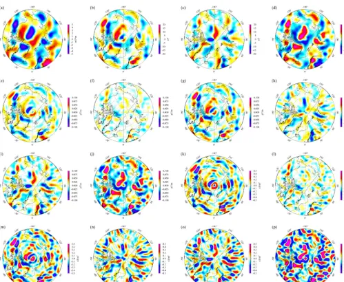
Figure 1. Lithospheric magnetic potential, magnetic vector and its gradient fields and third-order partial derivatives of the magnetic potential field around the North Pole (0◦≤θ≤30◦) at the altitude of 300 km as defined by the lithospheric magnetic field model GRIMM_L120 (version 0.0) (Lesur et al., 2013) for spherical harmonic degrees 16–90. (a) is magnetic potential (V ); (b), (c) and (d) are three components (Bx,ByandBz)of the magnetic vector; (e), (f), (g), (h), (i) and (j) are six elements (Bxx,Bxy,Bxz,Byy,Byz andBzz)of the magnetic gradient tensor; (k), (l), (m), (n), (o) and (p) are six elements (Bxxz,Bxyz,Bxzz,Byyz,ByzzandBzzz)of third-order partial derivatives of the magnetic potential field, respectively. The dark green lines are the plate boundaries by Bird (2003). All maps are shown in polar stereographic projections.

we also give the third-order partial derivatives of the mag-netic potential field as

Bxxz=∂Bxx

∂z = ∂2Bx

∂x∂z = ∂2Bx

∂z∂x

= 1 a2

L

P

l=1 l

P

m=0

(a_r)l+4 g_lmcosmφ+hm_l sinmφ

axxz_l,mPem −2 l +b

xxz

l,mPe_lm+cxxz_l,mPem +2 l

,

(28a)

Bxyz= ∂Bxy

∂z = ∂Byx

∂z = ∂2_Bx

∂y∂z= ∂2_Bx

∂z∂y = ∂2By

∂x∂z = ∂2By

∂z∂x

= 1 a2

L

P

l=1 l

P

m=0

(a_r)l+4 g_lmsinmφ−hm_l cosmφ

a_l,mxyzPe

m−2 l+1 +b

xyz l,mPe_lm₊₁+c

xyz l,mPe

m+2 l+1

,

(28b)

Bxzz=∂Bxz

∂z = ∂Bzx

∂z = ∂2Bx

∂z2 =

∂2_B z

∂x∂z = ∂2_B

z

∂z∂x

= 1 a2

L

P

l=1 l

P

m=0

(_ra)l+4 g_lmcosmφ+hm_l sinmφ

a_l,mxzzPe

m−1 l +b

xzz l,mPe

m+1 l

,

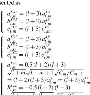
Table 1. Statistics of the magnetic potential, MV, MGT and third-order partial derivatives of the magnetic potential field around the North Pole (0◦≤θ≤30◦) at the altitude of 300 km using the lithospheric magnetic field model GRIMM_L120 (version 0.0) (Lesur et al., 2013) for spherical harmonic degrees 16–90.

Magnetic effects Minimum Maximum Mean Standard deviation

V (mT×m) −5.1554771 +4.7867519 +0.0828017 ±1.7377648

Bx(nT) -14.7389250 +17.6917740 -0.0890689 ±4.9797007

By(nT) −15.1297000 +13.6053000 +0.0010738 ±4.8239313

Bz(nT) −19.8715270 +25.3666030 −0.1988485 ±6.7066701

Bxx(pT m−1) −0.1054684 +0.0621351 +0.0001872 ±0.0215871

Bxy(pT m−1) −0.0410371 +0.0491030 +0.0000003 ±0.0115018

Bxz(pT m−1) −0.0929498 +0.1082861 +0.0006867 ±0.0247522

Byy(pT m−1) −0.0726248 +0.0505990 −0.0004789 ±0.0186580

Byz(pT m−1) −0.0868184 +0.0826627 +0.0000058 ±0.0228174

Bzz(pT m−1) −0.1015986 +0.1511038 +0.0002917 ±0.0336965

Bxx+Byy+Bzz(pT m−1) −2.012×10−15 +2.026×10−15 +8.085×10−19 ±5.101×10−16

Bxxz(aT m−2) −0.7589853 +0.4794999 +0.0002436 ±0.1537058

Bxyz(aT m−2) −0.2628265 +0.3734132 −0.0000004 ±0.0734794

Bxzz(aT m−2) −0.7067652 +0.8470055 +0.0140820 ±0.1752880

Byyz(aT m−2) −0.5259662 +0.4076568 −0.0134321 ±0.1370902

Byzz(aT m−2) −0.6058631 +0.6396412 +0.0000341 ±0.1448002

Bzzz(aT m−2) −0.7609268 +1.1697371 +0.0131885 ±0.2421663

Byyz= ∂Byy

∂z = ∂2By

∂y∂z = ∂2By

∂z∂y

= 1 a2

L

P

l=1 l

P

m=0

(a_r)l+4 g_lmcosmφ+hm_l sinmφ

ayyz_l,mPem −2 l +b

yyz l,mPe_lm+c

yyz l,mPem

+2 l

,

(28d)

Byzz= ∂Byz

∂z = ∂Bzy

∂z = ∂2By

∂z2 =

∂2Bz

∂y∂z= ∂2Bz

∂z∂y

= 1 a2

L

P

l=1 l

P

m=0

(a_r)l+4 g_lmsinmλ−hm_l cosmλ

ayzz_l,mPem −1 l−1 +b

yzz l,mPem

+1 l−1

,

(28e)

Bzzz=∂

2_B z

∂z2

= 1 a2

L

P

l=1 l

P

m=0 (a_r)l+4

g_lmcosmφ+hm_l sinmφ

a_l,mzzzPe_lm,

(28f)

where the corresponding coefficients of the SSALFs are pre-sented as

 



a_l,mxxz=(l+3) axx_l,m bxxz_l,m =(l+3) b_l,mxx cxxz_l,m =(l+3) cxx_l,m,

(29a)

 



a_l,mxyz=(l+3) a_l,mxy bxyz_l,m =(l+3) bxy_l,m cxyz_l,m =(l+3) c_l,mxy,

(29b)

       

      

a_l,mxzz=0.5(l+2) (l+3) √

l+m √

l−m+1√Cm/Cm−1 =(l+2) (l+3) ax_l,m=(l+3) a_l,mxz bxzz_l,m= −0.5(l+2) (l+3) √

l+m+1 √

l−m√Cm/Cm+1 =(l+2) (l+3) bx_l,m=(l+3) b_l,mxz,

(29c)

 



a_l,myyz=(l+3) ayy_l,m byyz_l,m =(l+3) byy_l,m c_l,myyz=(l+3) cyy_l,m,

(29d)

   

  

a_l,myzz=0.5(l+2) (l+3) √

l+m √

l+m−1√Cm/Cm−1 =_(l+2) (l+3) ay_l,m=_(l+3) a_l,myz

byzz_l,m=0.5(l+2) (l+3) √

l−m √

l−m−1√Cm/Cm+1 =(l+2) (l+3) by_l,m=(l+3) b_l,myz ,

(29e) a_l,mzzz= −(l+1) (l+2) (l+3)=(l+3) a_l,mzz

=(l+2) (l+3) a_l,mz . (29f)

In this way, we avoid computing recursively the SSALFs with singular terms, their first- and second-order derivatives as in the traditional formulae. The cost is only to calculate two additional degrees and orders for the SSALFs at most. It should be noted that, in this study, we use the conventional form of SSALF that ifm <0, thenPe_lm=(−1)|m|Pe

|m|

l and if

m > l, thenPe_lm=0.

3 Numerical investigation and discussion

Table 2. Statistics of the magnetic potential, MV, MGT and third-order partial derivatives of the magnetic potential field around the South Pole (150◦≤θ≤180◦) at the altitude of 300 km using the lithospheric magnetic field model GRIMM_L120 (version 0.0) (Lesur et al., 2013) for spherical harmonic degrees 16–90.

Magnetic effects Minimum Maximum Mean Standard deviation

V (mT×m) −3.3267455 +4.6543369 +0.0801853 ±1.2427083

Bx(nT) −11.440070 +15.9109730 +0.3451248 ±3.5403285

By(nT) −9.1169009 +15.0436160 −0.0001605 ±3.1560093

Bz(nT) −22.202857 +14.5020010 −0.3022955 ±4.7971494

Bxx(pT m−1) −0.0579914 +0.0704617 +0.0000845 ±0.0166266

Bxy(pT m−1) −0.0364002 +0.0308075 −0.0000006 ±0.0074702

Bxz(pT m−1) −0.0741850 +0.0831062 +0.0019925 ±0.0187492

Byy(pT m−1) −0.0569493 +0.0706456 +0.0019055 ±0.0143289

Byz(pT m−1) −0.0599346 +0.0897167 −0.0000012 ±0.0154623

Bzz(pT m−1) −0.1367168 +0.0735795 −0.0019900 ±0.0258066

Bxx+Byy+Bzz(pT m−1) −1.027×10−15 +2.012×10−15 +1.113×10−18 ±5.059×10−16

Bxxz(aT m−2) −0.4605216 +0.5307263 +0.0011232 ±0.1328515

Bxyz(aT m−2) −0.2840344 +0.2947601 −0.0000015 ±0.0526629

Bxzz(aT m−2) −0.5686811 +0.5634376 0.0181792 ±0.1497829

Byyz(aT m−2) −0.4262850 +0.5819095 +0.0186968 ±0.1169641

Byzz(aT m−2) −0.6194116 +0.6520948 −0.0000118 ±0.1085051

Bzzz(aT m−2) −1.0199774 +0.5863084 −0.0198200 ±0.2084566

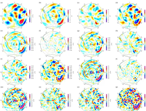
by Lesur et al. (2013). The magnetic potential, MV, MGT and the third-order partial derivatives of the magnetic po-tential field in the two polar regions mapped by the litho-spheric field model with litho-spherical harmonic degrees 16–90 are shown in Fig. 1 and Fig. 2, respectively. The correspond-ing statistics around the North Pole and South Pole are, re-spectively, presented in Tables 1 and 2. A simple test is that the MGT meets Laplace’s equation of the potential field; that is, the trace of the MGT should be equal to zero. Our nu-merical results show that the amplitudes ofBxx+Byy+Bzz

in the North Pole and South Pole regions are in the range of [−2.012×10−15pT m−1 to +2.026×10−15pT m−1] (1 Tesla =103mT=109 nT=1012 pT=1018aT), respec-tively. The relative error is almost equal to the machine’s accuracy. Therefore, this feature proves the validity of our derived formulae. In addition, as shown in Figs. 1 and 2, it is obvious that the MGT and also the third-order partial derivatives of the magnetic potential field enhance the lin-eation and contacts at the satellite altitude. It also reveals some small-scale anomalies, which is very helpful for further geological interpretation. A core field model with spherical harmonic degrees/orders 1–15 is also used for testing and the results, not shown here, indicate the correctness of the formu-lae in the full range of the spherical harmonic degrees/orders, where the computational stability of the Legendre function with ultrahigh-order is not considered.

Furthermore, the computed magnetic fields are smooth near the poles and do not have the singularities, but some components have the dependence on the direction of the ref-erence frame at the poles. As shown in Fig. 3, the magnetic potential V, the Bz,Bzz andBzzz components at the poles

are independent of the direction of thexPandyPaxes; while changing with the direction of thexPandyPaxes at the poles, theBx,By,Bxz,Byz,BxzzandByzzcomponents have a

pe-riod of 360◦ and theBxx,Bxy, Byy, Bxxz,Bxyz and Byyz

components have a period of 180◦. These variations can be accurately described by a sine or cosine function relating to the horizontal rotation of the reference frame and the dif-ferences among these magnetic effects are magnitude, pe-riod and initial phase. Therefore, theBx,By,Bxz,Byz,Bxx,

Bxy,Byy,Bxzz,ByzzBxxz,BxyzandByyzcomponents are not

smooth at/across the poles. Moreover, to determine the sin-gle value at the poles (Figs. 1, 2) we specially define that the x axis points to the meridian of 180◦E (or 180◦W) at the North Pole and of 0◦at the South Pole, that is, the LNORF moving from Greenwich meridian to the poles.

Figure 2. Lithospheric magnetic potential, magnetic vector and its gradient fields and third-order partial derivatives of the magnetic potential field around the South Pole (150◦≤θ≤180◦) at the altitude of 300 km as defined by the lithospheric magnetic field model GRIMM_L120 (version 0.0) (Lesur et al., 2013) for spherical harmonic degrees 16–90. (a) is magnetic potential (V ), (b), (c) and (d) are three components (Bx,By andBz)of the magnetic vector; (e), (f), (g), (h), (i) and (j) are six elements (Bxx,Bxy,Bxz,Byy,ByzandBzz)of the magnetic gradient tensor; (k), (l), (m), (n), (o) and (p) are six elements (Bxxz,Bxyz,Bxzz,Byyz,ByzzandBzzz)of third-order partial derivatives of the magnetic potential field, respectively. The dark green lines are the plate boundaries by Bird (2003). All maps are shown in polar stereographic projections.

of the three components Bx, By and Bz are at a level of

[−3×10−11nT to+3×10−11nT].

4 Conclusions

We develop in this paper the new expressions for the MV, the MGT and the third-order partial derivatives of the mag-netic potential field in terms of spherical harmonics. The tra-ditional expressions have complicated forms involving first-and second-order derivatives of the SSALFs first-and are singu-lar when approaching the poles. Our newly derived formulae do not contain the first- and second-order derivatives of the SSALFs and remove the singularities at the poles. However,

Figure 3. Limit values of the magnetic potential (V ), magnetic vector (Bx,ByandBz)and its gradients (Bxx,Bxy,Bxz,Byy,ByzandBzz) and third-order partial derivatives of the magnetic potential field (Bxxz,Bxyz,Bxzz,Byyz,ByzzandBzzz)at the poles when the local reference frames vary from different meridians (the direction ofxPaxes changing from different meridians to the poles). Red and blue lines indicate

the magnetic effects at the North Pole and at the South Pole, respectively. The reference frame is specially defined that thexPaxis points

to the meridian of 180◦E (or 180◦W) at the North Pole and 0f 0◦at the South Pole and theyPaxis points to the meridian of 90◦E at both

poles. The values at both poles shown by black dashed arrows are used to plot the maps in Figs. 1 and 2.

Code availability

Supplementary software implementation is performed with the programming language C/C++. The source code and in-put data presented in this paper can be obtained by contact-ing the correspondcontact-ing author via email or download from the Supplement related to the online version of this article.

The Supplement related to this article is available online at doi:10.5194/gmd-8-1979-2015-supplement.

Acknowledgements. This study is supported by the International

of Geosciences, Wuhan) (grant no. SMIL-2015-06) and State Key Laboratory of Geodesy and Earth’s Dynamics (Institute of Geodesy and Geophysics, CAS) (grant no. SKLGED2015-5-5-EZ). Jinsong Du is sponsored by the China Scholarship Council (CSC). We would like to thank Mehdi Eshagh and another anonymous reviewer for their constructive comments. All projected figures are drawn using the Generic Mapping Tools (GMT) (Wessel and Smith, 1991).

The article processing charges for this open-access publication were covered by a Research

Centre of the Helmholtz Association.

Edited by: L. Gross

References

Backus, G. E., Parker, R., and Constable, C.: Foundations of Geo-magnetism, Cambridge University Press, Cambridge, 1996. Bird, P.: An updated digital model of plate boundaries, Geochem.

Geophys. Geosyst., 4, 1027, doi:10.1029/2001GC000252, 2003. Blakely, R. G.: Potential Theory in Gravity and Magnetic

Applica-tions, Cambridge University Press, New York, 1995.

Blakely, R. J. and Simpson, R. W.: Approximating edges of source bodies from magnetic or gravity anomalies, Geophysics, 51, 1494–1498, 1986.

Eshagh, M.: Non-singular expressions for the vector and gradient tensor of gravitation in a geocentric spherical frame, Comput. Geosci., 34, 1762–1768, 2008.

Eshagh, M.: Alternative expressions for gravity gradients in local north-oriented frame and tensor spherical harmonics, Acta Geo-phys., 58, 215–243, 2009.

Finlay, C. C., Maus, S., Beggan, C. D., Bondar, T. N., Chambodut, A., Chernova, T. A., Chulliat, A., Golovkov, V. P., Hamilton, B., Hamoudi, M., Holme, R., Hulot, G., Kuang, W., Langlais, B., Lesur, V., Lowes, F. J., Lühr, H., Macmillan, S., Mandea, M., McLean, S., Manoj, C., Menvielle, M., Michaelis, I., Olsen, N., Rauberg, J., Rother, M., Sabaka, T. J., Tangborn, A., Tøffner-Clausen, L., Thébault, E., Thomson, A. W. P., Wardinski, I., Wei, Z., and Zvereva, T. I.: International Geomagnetic Reference Field: the eleventh generation, Geophys. J. Int., 183, 1216–1230, 2010.

Friis-Christensen, E., Lühr, H., and Hulot, G.: Swarm: A constella-tion to study the Earth’s magnetic field, Earth Planet. Space, 58, 351–358, 2006.

Gauss, C. F.: Allgemeine Theorie des Erdmagnetismus, in: Resul-tate aus den Beobachtungen des magnetischen vereins im Jahre 1838, edited by: Gauss, C. F. and Weber, W., (Leipzig, 1839), 1–57, 1838.

Golynsky, A., Bell, R., Blankenship, D., Damaske, D., Ferracci-oli, F., Finn, C., Golynsky, D., Ivanov, S., Jokat, W., Masolov, V., Riedel, S., von Frese, R., Young, D., and ADMAP Working Group: Air and shipborne magnetic surveys of the Antarctic into the 21st century, Tectonophysics, 585, 3–12, 2013.

Harrison, C. and Southam, J.: Magnetic field gradients and their uses in the study of the Earth’s magnetic field, J. Geomagn. Geo-electr., 43, 485–599, 1991.

Holmes, S. A. and Featherstone, W. E.: A unified approach to the Clenshaw summation and the recursive computation of very high

degree and order normalized associated Legendre functions, J. Geodynam., 76, 279–299, 2002a.

Holmes, S. A. and Featherstone, W. E.: SHORT NOTES: extending simplified high-degree synthesis methods to second latitudinal derivatives of geopotential, J. Geodynam., 76, 447–450, 2002b. Hsu, S. K., Sibuet, J. C., and Shyu, C. T.: High-resolution

detec-tion of geologic boundaries from potential-field anomalies: An enhanced analytic signal technique, Geophysics, 61, 373–386, 1996.

Ilk, K. H.: Ein eitrag zur Dynamik ausgedehnter Körper-Gravitationswechselwirkung, Deutsche Geodätische Kommis-sion. Reihe C, Heft Nr. 288, München, 1983.

Kotsiaros, S. and Olsen, N.: The geomagnetic field gradient tensor: Properties and parametrization in terms of spherical harmonics, Int. J. Geomath., 3, 297–314, 2012.

Kotsiaros, S. and Olsen, N.: End-to-End simulation study of a full magnetic gradiometry mission, Geophys. J. Int., 196, 100–110, 2014.

Kotsiaros, S., Finlay, C. C., and Olsen, N.: Use of along-track mag-netic field differences in lithospheric field modelling, Geophys. J. Int., 200, 878–887, 2015.

Langel, R. A. and Hinze, W. J.: The Magnetic Field of the Earth’s Lithosphere: The Satellite Perspective, Cambridge University Press, Cambridge, United Kingdom, 1998.

Langlais, B., Lesur, V., Purucker, M. E., Connerney, J. E. P., and Mandea, M.: Crustal Magnetic Fields of Terrestrial Planets, Space Sci. Rev., 152, 223–249, 2010.

Lesur, V., Rother, M., Vervelidou, F., Hamoudi, M., and Thébault, E.: Post-processing scheme for modelling the lithospheric mag-netic field, Solid Earth, 4, 105–118, doi:10.5194/se-4-105-2013, 2013.

Maus, S.: An ellipsoidal harmonic representation of Earth’s litho-spheric magnetic field to degree and order 720, Geochem. Geo-phys. Geosyst., 11, Q06015, doi:10.1029/2010GC003026, 2010. Maus, S., Yin, F., Lühr, H., Manoj, C., Rother, M., Rauberg, J., Michaelis, I., Stolle, C., and Müller, R. D.: Resolution of di-rection of oceanic magnetic lineations by the sixth-generation lithospheric magnetic field model from CHAMP satellite mag-netic measurements, Geochem. Geophys. Geosyst., 9, Q07021, doi:10.1029/2008GC001949, 2008.

Olsen, N. and the Swarm End-to-End Consortium: Swarm-End-to-End mission performance simulator study, ESA contract No. 17263/02/NL/CB, DSRI Report 1/2004, Danish Space Research Institute, Copenhagen, 2004.

Olsen, N., Hulot, G., and Sabaka, T. J.: Sources of the Geomagnetic Field and the Modern Data That Enable Their Investigation, in: Handbook of Geomathematics, edited by: Freeden, W., Nashed, M. Z., and Sonar, T., Springer, Netherlands, 106–124, 2010. Olsen, N., Lühr, H., Finlay, C. C., Sabaka, T. J., Michaelis, I.,

Rauberg, J., and Tøffner-Clausen, L.: The CHAOS-4 geomag-netic field model, Geophys. J. Int., 197: 815–827, 2014. Olsen, N., Hulot, G., Lesur, V., Finlay, C. C., Beggan, C., Chulliat,

Pedersen, L. B. and Rasmussen, T. M.: The gradient tensor of po-tential field anomalies: Some implications on data collection and data processing of maps, Geophysics, 55, 1558–1566, 1990. Petrovskaya, M. S. and Vershkov, A. N.: Non-singular expressions

for the gravity gradients in the local north-oriented and orbital reference frames, J. Geodynam., 80, 117–127, 2006.

Purucker, M., Sabaka, T., Le, G., Slavin, J. A., Strangeway, R. J., and Busby, C.: Magnetic field gradients from the ST-5 constella-tion: Improving magnetic and thermal models of the lithosphere, Geophys. Res. Lett., 34, L24306, doi:10.1029/2007GL031739, 2007.

Purucker, M. and Whaler, K.: Crustal magnetism, in: Treatise on Geophysics, vol. 5, Geomagnetism, edited by: Kono, M., Else-vier, Amsterdam, 195–237, 2007.

Purucker, M. E.: Lithospheric studies using gradients from close encounters of Ørsted, CHAMP and SAC-C, Earth Planet. Space, 57, 1–7, 2005.

Ravat, D.: Interpretation of Mars southern highlands high amplitude magnetic field with total gradient and fractal source modeling: New insights into the magnetic mystery of Mars, Icarus, 214, 400–412, 2011.

Ravat, D., Wang, B., Wildermuth, E., and Taylor, P. T.: Gradients in the interpretation of satellite-altitude magnetic data: an example from central Africa, J. Geodynam., 33, 131–142, 2002.

Sabaka, T. J., Tøffner-Clausen, L., and Olsen, N.: Use of the Com-prehensive Inversion method for Swarm satellite data analysis, Earth Planet. Space, 65, 1201–1222, 2013.

Sabaka, T. J., Olsen, N., Tyler, R. H., and Kuvshinov, A.: CM5, a pre-Swarm comprehensive magnetic field model derived from over 12 years of CHAMP, Ørsted, SAC-C and observatory data, Geophys. J. Int., 200, 1596–1626, 2015.

Schmidt, P. and Clark, D.: Advantages of measuring the magnetic gradient tensor, Preview, 85, 26–30, 2000.

Schmidt, P. and Clark, D.: The magnetic gradient tensor: its proper-ties and uses in source characterization, The Leading Edge, 25, 75–78, 2006.

Taylor, P. T., Kis, K. I., and Wittmann, G.: Satellite-altitude horizontal magnetic gradient anomalies used to define the Kursk magnetic anomaly, J. Appl. Geophys., 109, 133–139, doi:10.1016/j/jappgeo.2014.07.018, 2014.

Thébault, E., Purucker, M., Whaler, K. A., Langlais, B., and Sabaka, T. J.: The Magnetic Field of Earth’s Lithosphere, Space Sci. Rev., 155, 95–127, 2010.