www.geosci-model-dev.net/8/2815/2015/ doi:10.5194/gmd-8-2815-2015
© Author(s) 2015. CC Attribution 3.0 License.
POM.gpu-v1.0: a GPU-based Princeton Ocean Model
S. Xu1, X. Huang1, L.-Y. Oey2,3, F. Xu1, H. Fu1, Y. Zhang1, and G. Yang1
1Ministry of Education Key Laboratory for Earth System Modeling, Center for Earth System Science, Tsinghua University, 100084, and Joint Center for Global Change Studies, Beijing, 100875, China
2Institute of Hydrological & Oceanic Sciences, National Central University, Jhongli, Taiwan 3Program in Atmospheric & Oceanic Sciences, Princeton University, Princeton, New Jersey, USA
Correspondence to: X. Huang ([email protected])
Received: 13 October 2014 – Published in Geosci. Model Dev. Discuss.: 17 November 2014 Revised: 10 August 2015 – Accepted: 19 August 2015 – Published: 9 September 2015
Abstract. Graphics processing units (GPUs) are an attrac-tive solution in many scientific applications due to their high performance. However, most existing GPU conversions of climate models use GPUs for only a few computation-ally intensive regions. In the present study, we redesign the mpiPOM (a parallel version of the Princeton Ocean Model) with GPUs. Specifically, we first convert the model from its original Fortran form to a new Compute Unified Device Ar-chitecture C (CUDA-C) code, then we optimize the code on each of the GPUs, the communications between the GPUs, and the I/O between the GPUs and the central process-ing units (CPUs). We show that the performance of the new model on a workstation containing four GPUs is comparable to that on a powerful cluster with 408 standard CPU cores, and it reduces the energy consumption by a factor of 6.8.
1 Introduction
High-resolution atmospheric, oceanic and climate mod-ellings remain significant scientific and engineering chal-lenges because of the enormous computing, communication, and storage requirements involved. Due to the rapid develop-ment of computer architecture, in particular the developdevelop-ment of multi-core and many-core hardware, the computing power that can be applied to scientific problems has increased ex-ponentially in recent decades. Parallel computing methods, such as the Message Passing Interface (MPI, Gropp et al., 1999) and Open Multi-Processing (OpenMP, Chapman et al., 2008), have been widely used to support the parallelization of climate models. However, supercomputers are becoming in-creasingly heterogeneous, involving devices such as the GPU
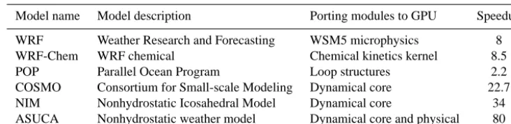
and the Intel Many Integrated Core (Intel MIC), and new ap-proaches are required to effectively utilize the new hardware. In recent years, a number of scientific codes have been ported to the GPU as shown in Table 1. Most existing GPU acceleration codes for climate models are only operating on certain hot spots of the program, leaving a significant portion of the program still running on CPUs. The speed of some subroutines reported in the Weather Research and Forecast (WRF) (Michalakes and Vachharajani, 2008) and WRF-Chem (Linford et al., 2009) is improved by a factor of approximately 8, whereas the whole model achieves lim-ited speedup because of partial porting. The speed of POP (Zhenya et al., 2010) is improved by a factor of only 2.2 be-cause the model only accelerated a number of loop structures using the OpenACC Application Programming Interface (OpenACC API). The speed of COSMO (Leutwyler et al., 2014), NIM (Govett et al., 2010) and ASUCA (Shimokawabe et al., 2010) are greatly improved by multiple GPUs. We be-lieve that the elaborate optimization of the memory access of each GPU and the communication between GPUs can further accelerate these models.
Table 1. Existing GPU porting work in climate fields. The speedups are normalized to one CPU core.
Model name Model description Porting modules to GPU Speedup
WRF Weather Research and Forecasting WSM5 microphysics 8
WRF-Chem WRF chemical Chemical kinetics kernel 8.5
POP Parallel Ocean Program Loop structures 2.2
COSMO Consortium for Small-scale Modeling Dynamical core 22.7
NIM Nonhydrostatic Icosahedral Model Dynamical core 34
ASUCA Nonhydrostatic weather model Dynamical core and physical 80
GPUs and the CPUs to further improve the performance of POM.gpu.
To understand the accuracy, performance and scalability of the POM.gpu code, we customized a workstation with four Nvidia K20X GPUs. The results show that the performance of POM.gpu running on this workstation is comparable to that on a powerful cluster with 408 standard CPU cores.
This paper is organized as follows. In Sect. 2, we review the mpiPOM model. In Sect. 3, we briefly introduce the GPU computing model. In Sect. 4, we present the detailed opti-mization techniques. In Sect. 5, we report on the correctness, performance and scalability of the model. We present the code availability in Sect. 6 and conclude our work in Sect. 7.
2 The mpiPOM
The mpiPOM is a parallel version of the POM. It retains most of the physics of the original POM (Blumberg and Mellor, 1983, 1987; Oey et al., 1985a, b, c; Oey and Chen, 1992a, b) and includes satellite and drifter assimilation schemes from the Princeton Regional Ocean Forecast System (Oey, 2005; Lin et al., 2006; Yin and Oey, 2007), stokes drift and wave-enhanced mixing (Oey et al., 2013; Xu et al., 2013; Xu and Oey, 2014). The POM code was reorganized and the parallel MPI version was implemented by Jordi and Wang (2012) us-ing a two-dimensional data decomposition of the horizontal domain. The MPI is a standard library for message passing and is widely used to develop parallel programs. The POM is a powerful ocean model that has been used in a wide range of applications: circulation and mixing processes in rivers, estu-aries, shelves, slopes, lakes, semi-enclosed seas and open and global oceans. It is also at the core of various real-time ocean and hurricane forecasting systems, e.g. the Japanese coastal ocean and Kuroshio current (Miyazawa et al., 2009; Isobe et al., 2012; Varlamov et al., 2015), the Adriatic Sea Fore-casting System (Zavatarelli and Pinardi, 2003), the Mediter-ranean Sea forecasting system (Korres et al., 2007), the GFDL Hurricane Prediction System (Kurihara et al., 1995, 1998), the US Hurricane Forecasting System (Gopalakrish-nan et al., 2010, 2011), and the Advanced Taiwan Ocean Prediction (ATOP) system (Oey et al., 2013). Additionally, the model has been used to study various geophysical fluid dynamical processes (e.g. Allen and Newberger, 1996;
New-berger and Allen, 2007a, b; Kagimoto and Yamagata, 1997; Guo et al., 2006; Oey et al., 2003; Zavatarelli and Mellor, 1995; Ezer and Mellor, 1992; Oey, 2005; Xu and Oey, 2011, 2014, 2015; Chang and Oey, 2014; Huang and Oey, 2015; Sun et al., 2014, 2015). For a more complete list, please visit the POM website (http://www.ccpo.odu.edu/POMWEB).
The mpiPOM experiment used in this paper is one of two that were designed and tested by Professor Oey and students; the codes and results are freely available at the FTP site (ftp:// profs.princeton.edu/leo/mpipom/atop/tests/). The reader can refer to Chapter 3 of the lecture notes (Oey, 2014) for more detail. The test case is a dam-break problem in which warm and cold waters are initially separated in the middle of a zonally periodic channel (200 km×50 km×50 m) on an f-plane, with walls at the northern and southern boundaries. Geostrophic adjustment then ensues and baroclinic instabil-ity waves amplify and develop into finite-amplitude eddies in 10∼20 days. The horizontal grid sizes are 1 km and there are 50 vertical sigma levels. Although the problem is a test case, the code is the full mpiPOM version used in the ATOP forecasting system.
The main computational problem of the mpiPOM is mem-ory bandwidth limited. To confirm this issue, we use the run-time performance API tool to estimate the floating point op-eration count and the memory access instruction count, as in Browne et al. (2000). The results reveal that the computa-tional intensity, defined as floating point operations per byte transferred to or from memory, of the mpiPOM is approxi-mately 1:3.3, whereas the computational intensity provided by a modern high-performance CPU (an Intel SandyBridge E5-2670) is 7.5:1. Many large arrays are mostly pulled from the main memory and there is poor data reuse in the mpiPOM. In addition, there are no obvious hot spot func-tions in the mpiPOM, and even the most time-consuming subroutine occupies only 20 % of the total execution time. Therefore, porting a handful of subroutines to the GPU is not helpful in improving the model efficiency. This explains why we must port the entire program from the CPU to the GPU.
3 GPU computing model overview
Modern GPUs employ a stream-processing model with par-allelism. Each GPU contains a number of stream multipro-cessors (SMs). In this work, we carried out the conversion using four Nvidia K20X GPUs. Each K20X GPU contains 14 SMs and each SM has 192 single-precision processors and 64 additional processors for double precision. Although the computational capability of each processor is low, one GPU with thousands of processors can greatly boost the performance compared to the CPU. In computing, FLOPS (FLoating-point Operations Per Second) is a measure of computer performance. The theoretical peak performance of each K20X GPU is 3.93 teraFLOPS (TFLOPS, one trillion floating-point operations per second) for the single-precision floating-point calculations. In contrast, a single Intel Sandy-Bridge E5-2670 CPU is only capable of 0.384 TFLOPS.
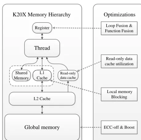
Each pair of GPUs shares 6 Gigabytes (GB) of mem-ory, with the interface having a potential bandwidth of 250 GB s−1. Figure 3 illustrates the memory hierarchy of the K20X GPU. Each SM possesses some types of fast on-chip memory such as register, L1 cache, shared memory and read-only data cache. In GPUs, the register is the fastest memory, of which the size is 256 Kilobytes (KB) for each SM. The shared memory and the L1 cache use the common 64 KB space, which can be partitioned as 16/48 KB, 32/32 KB or 48/16 KB. The 48 KB read-only data cache is useful for hold-ing frequently used values that remain unchanged durhold-ing each stage of the processing.
There are three widely used methods for porting a program to GPUs. The first method uses drop-in libraries provided by CUDA to replace the existing code, as in Siewertsen et al. (2013). The second method uses the OpenACC directive as hints in the original CPU code as in Zhenya et al. (2010). The last method is the most complex but also the most effective; it
kernel 1 kernel 3
kernel 0 kernel 2
Time
stream 0
stream 1
...
...
...
...
...
...
...
...
...
...
...
...
... ... thread
kernel
GPU
block(0,0) block(1,0) block(2,0)
block(0,1) block(1,1) block(2,1) warp block
warp
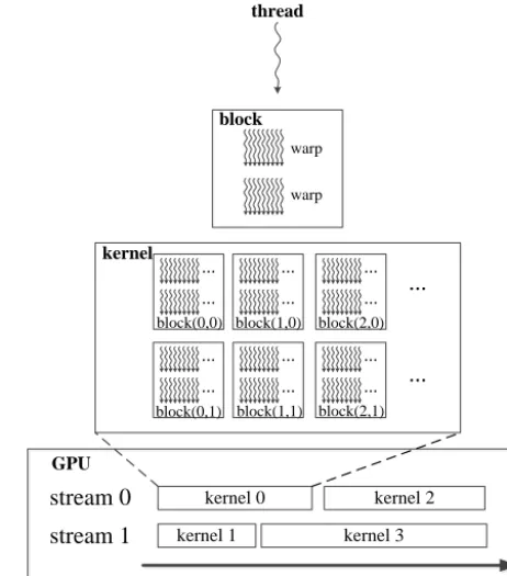
Figure 1. The hierarchy of stream, kernel, block, warp and thread.
involves rewriting the entire program using low-level CUDA subroutines.
In CUDA terminology, a kernel is a single section of code or subroutine running on the GPU. The underlying code in a kernel is split into a series of threads, each of which deals with different data. These threads are grouped into equal-size thread blocks that can be executed independently. A thread block is further divided into warps as basic scheduled units. A warp consists of 32 consecutive threads that execute the same instruction simultaneously. Each kernel and data trans-fer command in CUDA has an optional parameter, “stream ID”. If the stream ID is set in code, commands belonging to different streams can be executed concurrently. A stream in CUDA is a sequence of commands executed in order. Differ-ent streams can execute concurrDiffer-ently with differDiffer-ent priorities. Figure 1 illustrates the hierarchy of these terms.
4 Full GPU acceleration of the mpiPOM
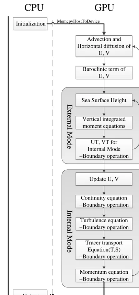
Figure 2 is a flowchart illustrating the structure of the POM.gpu. The main difference between the mpiPOM and the POM.gpu is that the CPU in the POM.gpu is only respon-sible for the initializing and the output work. The POM.gpu begins by initializing the relevant arrays on the CPU and then copies data from the CPU to the GPU. The GPU then per-forms all of the model computations. Outputs such as veloc-ity and sea-surface height (SSH) are copied back to the CPU and are then written to the disk at a user-specified time inter-val.
In the following sections, we introduce the optimizations of the POM.gpu by computation, communication and I/O aspects individually.
For the individual GPUs, we concentrate on memory ac-cess optimization by making better use of caches in the GPU memory hierarchy. This involves using read-only data cache, local memory blocking, loop fusion and function fusion, and disabling error-correcting code memory. The test results demonstrate that a single GPU can run the model almost 100 times faster than a single CPU core.
In terms of communication, we overlapped the sending of boundary data between the GPUs with the main computation. Data are also sent directly between the GPUs, bypassing the CPU.
In terms of I/O, we launched extra MPI processes on the main CPU to output the data. These MPI processes are di-vided into two categories, the computation processes and the I/O processes. The computation processes are responsible for launching kernels into GPUs and the I/O processes are responsible for copying data back from the GPUs and for writing to disks. The computation processes and the I/O processes can execute simultaneously to save output time.
4.1 Computational optimizations in a single GPU Managing the significant performance difference between global memory and on-chip fast memory is the primary con-cern for GPU computing. The ratio of bandwidth between global memory and shared memory is approximately 1:10. Therefore, data reuse in an on-chip cache always needs to be seriously considered. As shown on the right side of Fig. 3, we propose two classes of optimization, including the stan-dard optimization of fusion and the special optimization of the GPU, to better utilize the fast registers and caches.
4.1.1 Standard optimizations of fusion
Fusion optimization in the POM.gpu code includes loop fu-sion and function fufu-sion. The loop fufu-sion merges several loops into one loop and the function fusion merges several subroutines into one subroutine.
Loop fusion is an effective method to store scalar variables in registers for data reuse. As shown in Fig. 4, if the variable
Initialization
Output
Advection and Horizontal diffusion of
U, V
Baroclinic term of U, V
Sea Surface Height
Vertical integrated moment equations
UT, VT for Internal Mode +Boundary operation
Update U, V
Continuity equation +Boundary operation
Turbulence equation +Boundary operation
Tracer transport Equation(T,S) +Boundary operation
Momentum equation +Boundary operation
E
x
te
rn
al
M
o
d
e
In
te
rn
al
M
o
d
e
CPU
GPU
MemcpyDeviceToHost MemcpyHostToDevice
Figure 2. POM.gpu flowchart.
drhox(k, j, i) is read several times in multiple loops, we can
fuse these loops into one. Therefore, drhox(k, j, i) will first be read from the global memory and then repeatedly read from a register. For instance, for the profq kernel optimized with loop fusion, the device memory transactions decrease by 57 %, and the running speed of this kernel is improved by 28.6 %. The loop fusion optimization can also be applied in a number of mpiPOM subroutines.
Thread
L1 Cache Shared
Memory
Read-only data cache
L2 Cache
Global memory
L1 Cache L1 CacheL1 Cache
Register Loop Fusion & Function Fusion
Read-only data cache utilization
Local memory Blocking
ECC-off & Boost
K20X Memory Hierarchy Optimizations
Figure 3. The memory hierarchy of the K20X GPU and the
rela-tionships with each optimization.
the advection terms in horizontal directions, respectively. Af-ter merging them into one subroutine, the redundant memory access is avoided. The function fusion can also be applied in which one function is called several times to calculate differ-ent tracers. The proft function in the mpiPOM code is called twice – one for temperature and one for salinity. Their com-puting formulas are similar and some common arrays are ac-cessed. After function fusion, the running speed of the proft kernel is improved by 28.8 %.
4.1.2 Special optimizations of the GPU
Our special optimizations mainly focus on the improved uti-lization of the read-only data cache and the L1 cache on the GPU. It is useful to alleviate the bottleneck of memory band-width that is limited by using these fast on-chip caches.
There is a 48 KB read-only data cache in the K20X GPU. We can automatically use this as long as the read-only con-dition is met. In the POM.gpu, we simply add const __re-strict__ qualifiers into the parameter pointers to explicitly di-rect the compiler to implement the optimization. As an exam-ple, consider the calculations of advection and the horizontal diffusion terms. Because mpiPOM adopts the Arakawa C-grid, in the horizontal plane, updating the temperature (T) requires the velocity of longitude (u), the velocity of lati-tude (v) and the horizontal kinematic viscosity (aam) on the neighbouring grid points. In one kernel, the uandvarrays are accessed twice, and the aam array is accessed four times. After using the read-only data cache to improve the data lo-cality, the running speed of this kernel is improved by 18.8 %.
To reuse the data in each thread, we use local memory blocking to pull the data from global memory to the L1 cache. In this method, a small subset of a data set is loaded into the fast on-chip memory and then the small data block is repeatedly accessed by the program. This method is help-ful in reducing the need to access the off-chip with high la-tency memory. In the subroutines of the vertical diffusion and source/sink terms, the chasing method is used to solve a tridiagonal matrix along the vertical direction for each grid point individually. Each thread only accesses its own tiles of row transformation coefficients. As shown in Fig. 5, the arrays are accessed twice within one thread, one from the surface (k=0) to the bottom (k=nz−1) and another from the bottom (k=nz−1) to the surface (k=0). After blocking the vertical direction arrays in local memory, the L1 cache is fully utilized, and the running speed of these subroutines is improved by 35.3 %.
In the current implementation, as in the original mpiPOM code, the three-dimensional arrays of variables are stored se-quentially as east–west (x), north–south (y), and vertical (z), i.e.i, j, kordering. Two-dimensional arrays are stored ini, j ordering. The vertical diffusion is solved using a tridiagonal solver that is calculated sequentially in thezdirection. For simplicity, in our kernel functions the grid is divided along x andy. Each GPU thread then specifies an(x, y) point in the horizontal direction and performs all of the calculations from the surface to the bottom. The thread blocks are divided as 32×4 subdomains in the x–y plane. In the x direction, the block number must be a multiple of 32 threads to per-form consecutive and aligned memory access within a warp (NVIDIA, 2015). In they direction, we tested many thread numbers, such as 4 and 8, and obtained similar performances. We ultimately choose 4 because this value produced more blocks and allowed us to distribute the workload more uni-formly amongst the SMs. In addition, 128 (=32×4) threads are enough to maintain the full occupancy, which is the num-ber of active threads in each multiprocessor.
In GPU computing, one is free to choose which arrays will be stored in an on-chip cache. Our experience involves putting the data along the horizontal direction into the read-only cache to reuse among threads, and putting the data along with vertical direction into the local memory for reuse within one thread.
Furthermore, we improve the global memory bandwidth by disabling the Error Checking and memory Correcting (ECC-off), as well as enhancing the clock on the GPU (GPU boost). This method improves the performance of the POM.gpu by 13.8 %.
4.1.3 Results of the computational optimizations
opti-/*************************
*There exist two loops.
*drhox is visited twice in these loops. *************************/ for (k = 1; k < nz-1; k++){
drhox[k][j][i] = drhox[k-1][j][i] + A[k][j][i]; }
for (k = 0; k< nz-1; k++){
drhox[k][j][i] = drhox[k][j][i] * B[k][j][i]; }
/*************************
*These loops can be fused into one
*to reduce global memory access. *************************/ for (k = 1; k < nz-1; k++){
drhox[k][j][i] = drhox[k-1][j][i] + A[k][j][i]; drhox[k-1][j][i] = drhox[k-1][j][i] * B[k-1][j][i]; }
drhox[k-1][j][i] = drhox[k-1][j][i] * B[k-1][j][i];
(a)
Original CUDA-C code
(b)
Optimized CUDA-C code
Figure 4. A simple example of loop fusion.
/*************************
*3D arrays ee and gg represent row transformation *coefficients of the chasing method.
*************************/
for (k = 1; k < nz-2; k++){
ee[k][j][i] = ee[k-1][j][i]*A[k][j][i];
gg[k][j][i] = ee[k-1][j][i]*gg[k-1][j][i] - B[k][j][i]; }
for (k = nz-3; k>= 0; k++){
uf[k][j][i] = (ee[k][j][i]*uf[k+1][j][i]+gg[k]) * C[k][j][i]; }
/*************************
*Each thread pulls its own tile of ee,gg to *1D new arrays ee_new, gg_new(local memory). *There two new arrays can be cached in L1 for reuse.
*************************/
for (k = 1; k < nz-2; k++){
ee_new[k] = ee_new[k-1]*A[k][j][i]; gg_new[k] = ee_new[k-1]*gg[k-1] - B[k][j][i]; }
for (k = nz-3; k>= 0; k++){
uf[k][j][i] = (ee_new[k]*uf[k+1]+gg_new[k])*C[k][j][i]; }
(a)Original CUDA-C code (b)Optimized CUDA-C code
Figure 5. A simple example of local memory blocking.
mizations in these categories to improve the performance of POM.gpu; these categories are described as follows.
1. Category 1: advection and horizontal diffusion (adv) This category has six subroutines, and calculates the ad-vection, horizontal diffusion and the pressure gradient and Coriolis terms in the case of velocity. Here, it is possible to reuse data among adjacent threads, and the subroutines therefore benefit from using the read-only data cache. At the same time, the variables are calcu-lated in different loops or in different functions such that the loop fusion and function fusion optimizations are applied to this part as well.
2. Category 2: vertical diffusion (ver)
This category has four subroutines and calculates the vertical diffusion. In this part, the chasing method is used in the tridiagonal solver in the k direction. The main feature is that the data are accessed twice within one thread, once from the surface to the bottom and again from the bottom to the surface. The subroutines are significantly sped up after grouping thek-direction variable in the local memories.
3. Category 3: vorticity (vort), baroclinicity (baro), conti-nuity equation (cont) and equation of state (state) This category is less time-consuming than the two cate-gories described above, but it also benefits from our op-timizations. Because data reuse exists among threads, the use of a read-only data cache improves data local-ity. For the vort subroutine, there is data reuse within one thread, and thus the loop fusion improves the data locality.
4.2 Communication optimizations among multiple GPUs
Table 2. Different subroutines adopt different optimizations in the POM.gpu.
Subroutines Loop Function Read-only Local memory ECC-off and Speedup
fusion fusion data cache blocking GPU boost
Adv. and hor. diff. √ √ √ √ 2.05X
Ver. diff. √ √ √ √ 2.82X
Baroclinicity √ √ √ 2.08X
Continuity equation √ √ 1.39X
Vorticity √ √ √ 3.19X
State equation √ √ 1.35X
Inner Region
(stream 1) North Region
(stream 2)
South Region
(stream 2)
W
es
t R
eg
io
n
(s
tr
ea
m
2
)
E
as
t R
eg
io
n
(s
tr
ea
m
2
)
W
es
t H
al
o
(s
tr
ea
m
2
)
E
as
t H
al
o
(s
tr
ea
m
2
)
North Halo(stream 3)
South Halo(stream 3)
32
Figure 6. Data decomposition in the POM.gpu.
(2010) and Yang et al. (2013) proposed fine-grained overlap-ping methods of GPU computation and CPU communication to improve the computing performance. An important issue in their work is that the communications between multiple GPUs explicitly require the participation of the CPU. In our current work, we simply bypass the CPU in implementing the communication to fully exploit the capability of the GPUs.
At present, two MPI libraries, OpenMPI and MVAPICH2, provide support for the direct communication from the GPU to the main memory. This capability is referred to as CUDA-aware MPI. We attempted to use MVAPICH2 to imple-ment direct communication among multiple GPUs. However, we found that inter-domain communication occupied nearly 18 % of the total runtime.
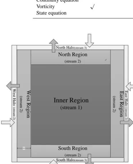
Instead, to fully overlap the boundary operations and MPI communications with computation, we adopt the data composition method shown in Fig. 6. The data region is de-composed into three regions: the inner region, the outer re-gion, and a halo region which exchanges data with its
neigh-bours. In our design, the inner region, which is the most time-consuming, is allocated to stream 1. The East/West outer re-gion is allocated to stream 2 and the North/South outer rere-gion is allocated to stream 3. In the East/West outer region, the width is set to 32 to ensure consecutive and aligned memory access in a warp. All of the halo regions are also allocated to stream 2.
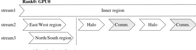
The workflow of multiple streams on the GPU is shown in Fig. 7. The East, West, North and South regions are com-mon kernel functions that can run in parallel with the inner region through different streams. The communication opera-tions between domains are implemented by an asynchronous CUDA memory copy. The corresponding synchronization operations between the CPU and the GPU or between the MPI processes are implemented by a synchronization CUDA function and a MPI barrier function. To overlap the subse-quent communication with the inner region, stream 2 and stream 3 for the outer region have higher priority in pre-empting the computing resource from stream 1 at any time. Based on this workflow, the inter-domain communication is overlapped with the computation. The experimental results show that our design can remove the communication over-head taken by MVAPICH2.
4.3 I/O optimizations between the GPUs and the CPUs
The time consumed for I/O in the mpiPOM is not signifi-cant. However, after we fully accelerate the model by GPU, it accounts for approximately 30 % of the total runtime. The computing phase and the I/O phase are serial, which means that the GPU will remain idle until the CPU finishes the I/O operations. Motivated by previous work on I/O overlapping (Huang et al., 2014), we designed a similar method follow-ing computations on a GPU and I/O operations on a CPU to run in parallel.
Rank0: GPU0
stream1
stream2
stream3
cudaStreamSynchronize Operation
Inner region
East/West region
North/South region
Halo Comm. Halo Comm.
Figure 7. The workflow of multiple streams on the GPU. The Inner/East/West/North/South regions and Halo refer to the computation and
update of the corresponding region. Comm. refers to the communication between processes, which implies synchronization.
Because the I/O processes must fetch data from the GPU, communication is necessary between them. The I/O pro-cesses obtain the device buffer pointers from the computing processes during the initialization phase. When writing his-tory files, the computing processes are blocked and remain idle for a short time, waiting for I/O processes to fetch data. Then, the computing processes continue their computation, and the I/O processes complete their output in the back-ground, as illustrated in Fig. 8. This method can be further optimized by placing the archive data in a set-aside buffer and carrying on the main calculation. However, the method requires more memory, which is not abundant in current K20X GPUs.
The advantage of this method is that it overlaps the I/O on the CPU with the model calculation on the GPU. In serial I/O, the GPU computing processes are blocked while data are sent to the CPU and written to disk. In overlapping I/O, the computing processes only wait for the data to be sent to the host. The bandwidth of data brought to the host is ap-proximately 6 GB s−1, but the output bandwidth to the disk is approximately 100 MB s−1, as determined by the speed of the disk. Therefore, the overlapping method significantly ac-celerates the entire application.
5 Experiments
In this section, we first describe the specification of our plat-form and comparison methodology to validate the correct-ness of the POM.gpu. Furthermore, we present the perfor-mance and scalability of the POM.gpu compared with the mpiPOM.
5.1 Platform setup
The POM.gpu runs in a workstation consisting of two CPUs and four GPUs. The CPUs are 2.6 GHz 8-core Intel Sandy-Bridge E5-2670. The GPUs are Nvidia Tesla K20X. The op-erating system is RedHat Enterprise Linux 6.3×86_64. All programs are complied with Intel compiler v14.0.1, CUDA 5.5 Toolkit, Intel MPI Library v4.1.3 and MVAPICH2 v1.9.
For comparison, the mpiPOM runs on the T ansuo100 cluster at Tsinghua University consisting of 740 nodes. Each
node is equipped with two 2.93 GHz 6-core Intel Xeon X5670 CPUs and 32 GB of memory. The nodes are con-nected through an InfiniBand network. The operating system is RedHat Enterprise Linux 5.5×86_64. Programs on this platform are compiled with Intel compiler v11.1 and Intel MPI v4.0.2. The mpiPOM code is compiled with its original compiler flags, i.e. “-O3 -fp-model precise”.
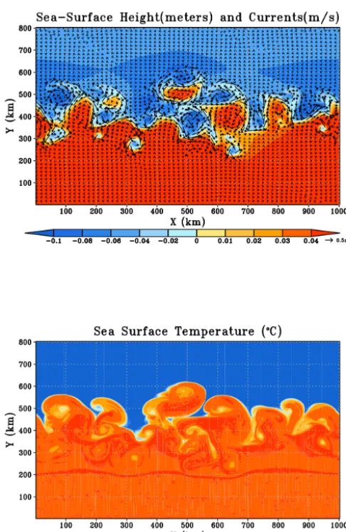
5.2 The test case and the verification of accuracy The “dam-break” simulation (Oey, 2014) is conducted to ver-ify the correctness and test the performance and scalability of the POM.gpu. It is a baroclinic instability problem that sim-ulates flows produced by horizontal temperature gradients. The model domain is configured as a straight channel with a uniform depth of 50 m. Periodic boundary conditions are used in the east–west direction, and the channel is closed in the north and south. Its horizontal resolution is 1 km×1 km. The domain size of this test case is 962×722 horizontal grid points and 51 vertical sigma levels, which is limited by the capacity of one’s GPU memory. Initially, the temperature in the southern half of the channel is 15 and 25◦C in the north-ern half. The salinity is fixed at 35 psu. The fluid is then allowed to adjust. In the first 3–5 days, geostrophic adjust-ments occur. Then, an unstable wave develops due to baro-clinic instability. Eventually, eddies are generated. Figure 9 shows the sea-surface height, sea-surface temperature (SST), and currents after 39 days. The scales of the frontal wave and eddies are determined by the Rossby radius of deformation. This dam-break case uses a single-precision format.
To verify the accuracy, we check the binary output files of the mpiPOM and the POM.gpu, as in Mak et al. (2011). The test results demonstrate that the variables velocity, tempera-ture, salinity and sea-surface height are all identical.
5.3 Model performance
One GPU
Compute process
I/O process
MPI_Barrier operation data
copy I/O
computation computation
data
copy I/O
computation
Time
Figure 8. One computing process and one I/O process both set their contexts on the same GPU. During the data copy phase, the computing process remains idle and the I/O process will copy data from the GPU to the CPU through thecudaMemcpyfunction.
Figure 9. The model results after 39 days of simulation. For the top
figure, the colour shading is the sea-surface height (SSH), and vec-tors are ocean currents. For the bottom figure, the colour shading is the sea-surface temperature (SST). Several warm and cold eddies are generated in the middle of the domain where the SST gradient is largest; their scales are determined by the Rossby radius of defor-mation.
0 50 100 150 200 250 300 350 400
20 30 40 50 60 70 80 90 100 110
Seconds per simulation day
CPU cores
One K20X GPU Intel X5670(6cores) Intel E5-2670(8 cores)
Figure 10. Performance comparison with different hardware
plat-forms.
5.3.1 Single GPU performance
0 20 40 60 80 100 120 140
1-GPU 2-GPUs 4-GPUs
Seconds per simulation day
Number of GPUs
Our design CUDA-aware MPI
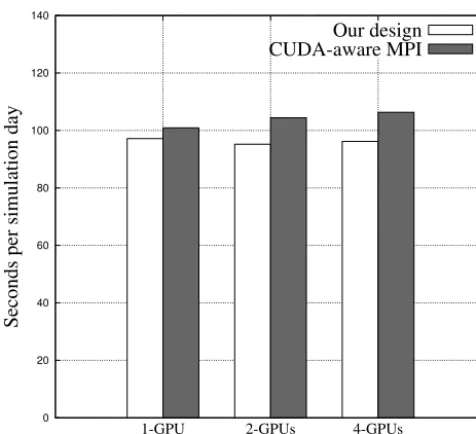
Figure 11. The weak scaling test between our communication
over-lapping method and the MVAPICH2 subroutines.
Table 3. The strong scaling result of POM.gpu.
Number of GPUs 1-GPU 2-GPUs 4-GPUs
Time (s) 97.2 48.7 26.3
Efficiency 100 % 99 % 92 %
5.3.2 Multiple GPU performance
In the second test, we compare our communication overlap-ping method with the MVAPICH2 library. Figure 11 presents the weak scaling performance on multiple GPUs, where the grid size for each GPU is kept at 962×722×51. When four GPUs are used with MVAPICH2, approximately 18 % of the total runtime is consumed by inter-domain communication and boundary operations. This overhead can be greatly re-duced by our communication overlapping method.
In the third test, we fix the global grid size at 962×722×
51, and measure the strong scaling performance of POM.gpu. Table 3 shows that the strong scaling efficiency is 99 % on two GPUs and 92 % on four GPUs. When more GPUs are used, the size of each subdomain becomes smaller. This de-creases the performance of POM.gpu in two aspects. First, the communication overhead may exceed the computation time of the inner region as the size of each subdomain de-creases. As a result, the overlapping methods in Sect. 4.2 are not effective. Second, there are many “small” kernels in the POM.gpu code, in which the calculation is simple and less time-consuming. With fewer inner region computations, the overhead of kernel launching and implicit synchronization with kernel execution must be counted.
0 200 400 600 800 1000 1200 1400 1600
1-GPU 2-GPUs 4-GPUs
Seconds of 20-days simulation
Number of GPUs
PnetCDF I/O-overlapping NO-I/O
Figure 12. I/O test for the POM.gpu.
5.3.3 I/O performance
In the fourth test, we compare our I/O overlapping method with the parallel NetCDF (PnetCDF) method and NO-I/O. NO-I/O means that all I/O operations are disabled in the program and that the time measured is the pure computing time. This simulation is run for 20 days, and the history files are output daily. The final history files in NetCDF format are approximately 12 GB. Figure 12 shows that the I/O overlap-ping method outperforms the PnetCDF method. For one and two GPUs, the overall runtime decreases from 1694/1142 to 1239/688 s, which is close to the NO-I/O. The extra over-head of our method compared with NO-I/O involves the computing processes that need to be blocked until the I/O processes obtain data from the GPUs. When running with four GPUs, the output time exceeds the computation time. Then, the I/O phase cannot be fully overlapped with the model computation phase. The overall runtime equals the sum of the computation time and the non-overlapped I/O time.
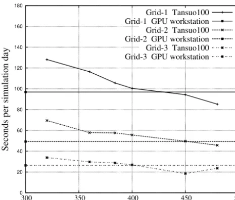
5.3.4 Comparison with a cluster
0 20 40 60 80 100 120 140 160 180
300 350 400 450 500
Seconds per simulation day
CPU cores
Grid-1 Tansuo100 Grid-1 GPU workstation Grid-2 Tansuo100 Grid-2 GPU workstation Grid-3 Tansuo100 Grid-3 GPU workstation
Figure 13. Performance test of four GPUs compared with the
Tan-suo100 cluster.
main of each MPI process becomes smaller, the cache hit ratio of the mpiPOM code will increase. This will greatly al-leviate the memory bandwidth-limited problem. However, in the simulation on 408 standard CPU cores, the MPI commu-nication may occupy more than 40 % of the total execution time. When scaling to over 450 cores, the mpiPOM simula-tion may instead become slower, as shown in Fig. 13. There-fore, for high-resolution ocean modelling, our POM.gpu has a clear advantage compared to the original mpiPOM.
6 Code availability
The POM.gpu version 1.0 is available at https://github.com/ hxmhuang/POM.gpu. To reproduce the test case in Sect. 5, the run_exp002.sh script is provided to compile and execute the POM.gpu code.
7 Conclusions and future work
In this paper, we develop POM.gpu, a full GPU solution based on the mpiPOM. Unlike previous GPU porting, the POM.gpu code distributes the model computations on the GPU. Our main contributions include optimizing the code on each of the GPUs, the communications between GPUs, and the I/O process between the GPUs and the CPUs. Us-ing a workstation with four GPUs, we achieve the perfor-mance of a powerful CPU cluster with 408 standard CPU cores. Our model also reduces the energy consumption by a factor of 6.8. It is a cost-effective and energy-efficient strat-egy for high-resolution ocean modelling. We have described the method and tests in detail and, with the availability of the POM.gpu code, our experiences may hopefully be useful to developers and designers of other general circulation models.
In our current POM.gpu, we design a large number of ker-nel functions because we port the entire mpiPOM one sub-routine at a time. This was done to simplify the debugging of POM.gpu and to check that the results are consistent with the mpiPOM. In our future work, we will adjust the code structure of POM.gpu and adopt aggressive function fusion to further improve the performance.
Previous studies proposed to take advantage of data lo-cality between time steps by time skewing (McCalpin and Wonnacott, 1999; Wonnacott, 2000), thus transforming the problem of memory bandwidth into the problem of compu-tation. However, the real-world ocean models, including the mpiPOM, often involve hundreds of thousands lines of code, and analysing the data dependency and applying time skew-ing in such a context are challengskew-ing and difficult. We leave that to the next-generation POM.gpu.
The Supplement related to this article is available online at doi:10.5194/gmd-8-2815-2015-supplement.
Acknowledgements. The author would like to thank David Webb,
Robert Marsh and the anonymous reviewer for their valuable comments and improvements regarding the presentation of this manuscript. This study was supported by funding from the National Natural Science Foundation of China (41375102), the National Grand Fundamental Research 973 Program of China (no. 2014CB347800), and the National High Technology Develop-ment Program of China (2011AA01A203).
Edited by: R. Marsh
References
Allen, J. S. and Newberger, P. A.: Downwelling Circulation on the Oregon Continental Shelf. Part I: Response to Idealized Forcing, J. Phys. Oceanogr., 26, 2011–2035, doi:10.1175/1520-0485(1996)026<2011:DCOTOC>2.0.CO;2, 1996.
Berntsen, J. and Oey, L.-Y.: Estimation of the internal pressure gradient inσ-coordinate ocean models: comparison of second-, fourth-second-, and sixth-order schemessecond-, Ocean Dynam.second-, 60second-, 317–330second-, 2010.
Blumberg, A. F. and Mellor, G. L.: Diagnostic and prognostic nu-merical circulation studies of the South Atlantic Bight, J. Geo-phys. Res.-Oceans, (1978–2012), 88, 4579–4592, 1983. Blumberg, A. F. and Mellor, G. L.: A description of a
three-dimensional coastal ocean circulation model, Coast. Est. Sci., 4, 1–16, 1987.
Browne, S., Dongarra, J., Garner, N., Ho, G., and Mucci, P.: A portable programming interface for performance evaluation on modern processors, Int. J. High Perf. Comp. Appl., 14, 189–204, 2000.
Chapman, B., Jost, G., and Van Der Pas, R.: Using OpenMP: portable shared memory parallel programming, vol. 10, The MIT Press, 2008.
Ezer, T. and Mellor, G. L.: A numerical study of the variability and the separation of the Gulf Stream, induced by surface atmo-spheric forcing and lateral boundary flows, J. Phys. Oceanogr., 22, 660–682, 1992.
Gopalakrishnan, S., Liu, Q., Marchok, T., Sheinin, D., Surgi, N., Tuleya, R., Yablonsky, R., and Zhang, X.: Hurricane Weather Re-search and Forecasting (HWRF) model scientific documentation, edited by: Bernardet, L., 75, 2010.
Gopalakrishnan, S., Liu, Q., Marchok, T., Sheinin, D., Surgi, N., Tong, M., Tallapragada, V., Tuleya, R., Yablonsky, R., and Zhang, X.: Hurricane Weather Research and Forecast-ing (HWRF) model: 2011 scientific documentation, edited by: Bernardet, L., 2011.
Govett, M., Middlecoff, J., and Henderson, T.: Running the NIM next-generation weather model on GPUs, in: Cluster, Cloud and Grid Computing (CCGrid), 2010 10th IEEE/ACM International Conference on, 792–796, IEEE, 2010.
Gropp, W. D., Lusk, E. L., and Thakur, R.: Using MPI-2: Advanced features of the message-passing interface, vol. 2, Globe Pequot, 1999.
Guo, X., Miyazawa, Y., and Yamagata, T.: The Kuroshio Onshore Intrusion along the Shelf Break of the East China Sea: The Origin of the Tsushima Warm Current, J. Phys. Oceanogr., 36, 2006. Henderson, T., Middlecoff, J., Rosinski, J., Govett, M., and
Mad-den, P.: Experience applying Fortran GPU compilers to numer-ical weather prediction, in: Application Accelerators in High-Performance Computing (SAAHPC), 2011 Symposium, 34–41, IEEE, 2011.
Huang, S.-M. and Oey, L.: Right-side cooling and phytoplank-ton bloom in the wake of a tropical cyclone, J. Geophys. Res.-Oceans, 2015.
Huang, X. M., Wang, W. C., Fu, H. H., Yang, G. W., Wang, B., and Zhang, C.: A fast input/output library for high-resolution climate models, Geosci. Model Dev., 7, 93–103, doi:10.5194/gmd-7-93-2014, 2014.
Isobe, A., Kako, S., Guo, X., and Takeoka, H.: Ensemble numerical forecasts of the sporadic Kuroshio water intrusion (kyucho) into shelf and coastal waters, Ocean Dyn., 62, 633–644, 2012. Jordi, A. and Wang, D.-P.: sbPOM: A parallel implementation of
Princenton Ocean Model, Environ. Model. Softw., 38, 59–61, 2012.
Kagimoto, T. and Yamagata, T.: Seasonal transport variations of the Kuroshio: An OGCM simulation, J. Phys. Oceanogr., 27, 403– 418, 1997.
Korres, G., Hoteit, I., and Triantafyllou, G.: Data assimilation into a Princeton Ocean Model of the Mediterranean Sea using ad-vanced Kalman filters, J. Marine Syst., 65, 84–104, 2007. Kurihara, Y., Bender, M. A., Tuleya, R. E., and Ross, R. J.:
Improve-ments in the GFDL hurricane prediction system, Mon. Weather Rev., 123, 2791–2801, 1995.
Kurihara, Y., Tuleya, R. E., and Bender, M. A.: The GFDL hurri-cane prediction system and its performance in the 1995 hurrihurri-cane season., Mon. Weather Rev., 126, 1306–1322, 1998.
Leutwyler, D., Fuhrer, O., Cumming, B., Lapillonne, X., Gysi, T., Lüthi, D., Osuna, C., and Schär, C.: Towards Cloud-Resolving European-Scale Climate Simulations using a fully GPU-enabled
Prototype of the COSMO Regional Model, in: EGU General As-sembly Conference Abstracts, vol. 16, p. 11914, 2014.
Lin, X., Xie, S.-P., Chen, X., and Xu, L.: A well-mixed warm water column in the central Bohai Sea in summer: Effects of tidal and surface wave mixing, J. Geophys. Res.-Oceans, 111, C11017, doi:10.1029/2006JC003504, 2006.
Linford, J. C., Michalakes, J., Vachharajani, M., and Sandu, A.: Multi-core acceleration of chemical kinetics for simulation and prediction, in: Proceedings of the Conference on High Per-formance Computing Networking, Storage and Analysis, p. 7, ACM, 2009.
Mak, J., Choboter, P., and Lupo, C.: Numerical ocean modeling and simulation with CUDA, in: OCEANS 2011, 1–6, IEEE, 2011. McCalpin, J. and Wonnacott, D.: Time skewing: A value-based
ap-proach to optimizing for memory locality, Tech. rep., Technical Report DCS-TR-379, Department of Computer Science, Rugers University, 477–480, 1999.
Michalakes, J. and Vachharajani, M.: GPU acceleration of numeri-cal weather prediction, Parallel Proc. Lett., 18, 531–548, 2008. Miyazawa, Y., Zhang, R., Guo, X., Tamura, H., Ambe, D., Lee,
J.-S., Okuno, A., Yoshinari, H., Setou, T., and Komatsu, K.: Water mass variability in the western North Pacific detected in a 15-year eddy resolving ocean reanalysis, J. Oceanogr., 65, 737–756, 2009.
Newberger, P. and Allen, J. S.: Forcing a three-dimensional, hy-drostatic, primitive-equation model for application in the surf zone: 1. Formulation, J. Geophys. Res.-Oceans, (1978–2012), 112, 2007a.
Newberger, P. A. and Allen, J. S.: Forcing a three-dimensional, hy-drostatic, primitive-equation model for application in the surf zone: 2. Application to DUCK94, J. Geophys. Res.-Oceans, 112, 2007b.
NVIDIA: CUDA C Best Practices Guide, available at:
http://docs.nvidia.com/cuda/cuda-c-best-practices-guide/ index.html#coalesce%d-access-to-global-memory (last access: April 2015), 2015.
Oey, L., Chang, Y.-L., Lin, Y.-C., Chang, M.-C., Xu, F.-H., and Lu, H.-F.: ATOP-the Advanced Taiwan Ocean Prediction Sys-tem based on the mpiPOM Part 1: model descriptions, analyses and results, Terr Atmos Ocean Sci, 24, 2013.
Oey, L.-Y.: A wetting and drying scheme for POM, Ocean Mod-elling, 9, 133–150, 2005.
Oey, L.-Y.: Geophysical Fluid Modeling with the mpi ver-sion of the Princeton Ocean Model (mpiPOM). Lecture Notes, 70 pp., ftp://profs.princeton.edu/leo/lecture-notes/ OceanAtmosModeling/Notes/GFModellingUsingMpiPOM.pdf (last access: January 2014), 2014.
Oey, L.-Y. and Chen, P.: A model simulation of circulation in the northeast Atlantic shelves and seas, J. Geophys. Res.-Oceans, 97, 20087–20115, 1992a.
Oey, L.-Y. and Chen, P.: A nested-grid ocean model: With appli-cation to the simulation of meanders and eddies in the Norwe-gian Coastal Current, J. Geophys. Res.-Oceans, (1978–2012), 97, 20 063–20 086, 1992b.
Oey, L.-Y., Mellor, G. L., and Hires, R. I.: A three-dimensional sim-ulation of the Hudson-Raritan estuary. Part II: Comparison with observation, J. Phys. Oceanogr., 15, 1693–1709, 1985b. Oey, L.-Y., Mellor, G. L., and Hires, R. I.: A three-dimensional
sim-ulation of the Hudson-Raritan estuary. Part III: Salt flux analyses, J. Phys. Oceanogr., 15, 1711–1720, 1985c.
Oey, L.-Y., Lee, H.-C., and Schmitz, W. J.: Effects of winds and Caribbean eddies on the frequency of Loop Current eddy shed-ding: A numerical model study, J. Geophys. Res.-Oceans, 108, 3324, doi:10.1029/2002JC001698, 2003.
Shimokawabe, T., Aoki, T., Muroi, C., Ishida, J., Kawano, K., Endo, T., Nukada, A., Maruyama, N., and Matsuoka, S.: Proceedings of the International Conference for High Performance Computing, Networking, Storage and Analysis, 1–11, An 80-fold speedup, 15.0 TFlops full GPU acceleration of non-hydrostatic weather model ASUCA production code, 2010.
Siewertsen, E., Piwonski, J., and Slawig, T.: Porting marine ecosys-tem model spin-up using transport matrices to GPUs, Geosci. Model Dev., 6, 17–28, doi:10.5194/gmd-6-17-2013, 2013. Smolarkiewicz, P. K.: A fully multidimensional positive definite
advection transport algorithm with small implicit diffusion, J. Comp. Phys., 54, 325–362, 1984.
Sun, J., Oey, L., Xu, F., Lin, Y., Huang, S., and Chang, R.: The Influence of Ocean on Typhoon Nuri (2008), in: AGU Fall Meet-ing Abstr., 1, L3360, available at: http://adsabs.harvard.edu/abs/ 2014AGUFM.A33L3360S, 2014.
Sun, J., Oey, L.-Y., Chang, R., Xu, F., and Huang, S.-M.: Ocean response to typhoon Nuri (2008) in western Pacific and South China Sea, Ocean Dynam., 65, 735–749, 2015.
Varlamov, S. M., Guo, X., Miyama, T., Ichikawa, K., Waseda, T., and Miyazawa, Y.: M2 baroclinic tide variability modulated by the ocean circulation south of Japan, J. Geophys. Res.-Oceans, 2015.
Wonnacott, D.: Using time skewing to eliminate idle time due to memory bandwidth and network limitations, in: Parallel and Dis-tributed Processing Symposium, 2000. IPDPS 2000, Proceed-ings, 14th International, 171–180, IEEE, 2000.
Xu, F.-H. and Oey, L.-Y.: The origin of along-shelf pressure gradi-ent in the Middle Atlantic Bight, J. Phys. Oceanogr., 41, 1720– 1740, 2011.
Xu, F.-H. and Oey, L.-Y.: State analysis using the Local Ensemble Transform Kalman Filter (LETKF) and the three-layer circula-tion structure of the Luzon Strait and the South China Sea, Ocean Dynam., 64, 905–923, 2014.
Xu, F.-H. and Oey, L.-Y.: Seasonal SSH variability of the Northern South China Sea, J. Phys. Oceanogr., 45, 1595–1609, 2015. Xu, F.-H., Oey, L.-Y., Miyazawa, Y., and Hamilton, P.: Hindcasts
and forecasts of Loop Current and eddies in the Gulf of Mex-ico using local ensemble transform Kalman filter and optimum-interpolation assimilation schemes, Ocean Model., 69, 22–38, 2013.
Yang, C., Xue, W., Fu, H., Gan, L., Li, L., Xu, Y., Lu, Y., Sun, J., Yang, G., and Zheng, W.: A peta-scalable CPU-GPU algorithm for global atmospheric simulations, in: Proceedings of the 18th ACM SIGPLAN symposium on Principles and practice of paral-lel programming, 1–12, ACM, 2013.
Yin, X.-Q. and Oey, L.-Y.: Bred-ensemble ocean forecast of Loop Current and rings, Ocean Model., 17, 300–326, 2007.
Zavatarelli, M. and Mellor, G. L.: A numerical study of the Mediter-ranean Sea circulation, J. Phys. Oceanogr., 25, 1384–1414, 1995. Zavatarelli, M. and Pinardi, N.: The Adriatic Sea modelling sys-tem: a nested approach, Ann. Geophys., 21, 345–364, 10.5194/ angeo-21-345-2003, 2003.