https://doi.org/10.5194/gmd-10-4563-2017 © Author(s) 2017. This work is distributed under the Creative Commons Attribution 3.0 License.
A method to encapsulate model structural uncertainty in ensemble
projections of future climate: EPIC v1.0
Jared Lewis1, Greg E. Bodeker1, Stefanie Kremser1, and Andrew Tait2
1Bodeker Scientific, 42 Russell Street, Alexandra, 9320, New Zealand
2National Institute of Water and Atmospheric Research, Wellington, New Zealand
Correspondence:Jared Lewis ([email protected]) Received: 13 February 2017 – Discussion started: 24 February 2017
Revised: 17 October 2017 – Accepted: 19 October 2017 – Published: 15 December 2017
Abstract. A method, based on climate pattern scaling, has been developed to expand a small number of projections of fields of a selected climate variable (X) into an ensemble that encapsulates a wide range of indicative model struc-tural uncertainties. The method described in this paper is re-ferred to as the Ensemble Projections Incorporating Climate model uncertainty (EPIC) method. Each ensemble member is constructed by adding contributions from (1) a climatology derived from observations that represents the time-invariant part of the signal; (2) a contribution from forced changes in X, where those changes can be statistically related to changes in global mean surface temperature (Tglobal); and
(3) a contribution from unforced variability that is generated by a stochastic weather generator. The patterns of unforced variability are also allowed to respond to changes inTglobal.
The statistical relationships between changes in X (and its patterns of variability) and Tglobal are obtained in a
“train-ing” phase. Then, in an “implementation” phase, 190 simu-lations ofTglobalare generated using a simple climate model
tuned to emulate 19 different global climate models (GCMs) and 10 different carbon cycle models. Using the generated Tglobal time series and the correlation between the forced
changes in X andTglobal, obtained in the “training” phase,
the forced change in theXfield can be generated many times using Monte Carlo analysis. A stochastic weather generator is used to generate realistic representations of weather which include spatial coherence. Because GCMs and regional cli-mate models (RCMs) are less likely to correctly represent unforced variability compared to observations, the stochastic weather generator takes as input measures of variability de-rived from observations, but also responds to forced changes in climate in a way that is consistent with the RCM
projec-tions. This approach to generating a large ensemble of pro-jections is many orders of magnitude more computationally efficient than running multiple GCM or RCM simulations. Such a large ensemble of projections permits a description of a probability density function (PDF) of future climate states rather than a small number of individual story lines within that PDF, which may not be representative of the PDF as a whole; the EPIC method largely corrects for such poten-tial sampling biases. The method is useful for providing pro-jections of changes in climate to users wishing to investigate the impacts and implications of climate change in a prob-abilistic way. A web-based tool, using the EPIC method to provide probabilistic projections of changes in daily maxi-mum and minimaxi-mum temperatures for New Zealand, has been developed and is described in this paper.
1 Introduction
a single projection, or a small set of projections (Watterson et al., 2008). That said, if decision makers are presented with PDFs obtained from the same family of models, these may be biased by the assumptions and limitations inherent in a single family of models that do not explore the possible trajecto-ries seen in other model families. PDFs of future climate that consider a greater number of sources of uncertainty, includ-ing uncertainty resultinclud-ing from structural differences in the underlying models, provide more robust information needed for quantitative risk assessments, since the likelihood of any particular trajectory can be better estimated.
Exploring expected changes in extreme weather events also requires probabilistic simulations of future climate. While climate change may result in a small shift in the mean and/or standard deviation (SD) of a PDF of a selected climate variable, the tails of the distribution, which represent extreme weather events, can exhibit fractionally much larger changes (see Fig. 1.8 in Solomon et al., 2007). It is especially impor-tant that extreme events, which by their nature are unusual, are captured in an ensemble of projections.
Resolving changes in the frequency of regional-scale ex-treme weather events requires large ensembles of projections of high spatial and temporal resolution. Generating such en-sembles using models which simulate all important physical processes, such as global climate models (GCMs) or regional climate models (RCMs), is currently computationally pro-hibitive. The ideas underlying climate pattern scaling sug-gest a means of overcoming this hurdle and form the basis for the newly developed Ensemble Projections Incorporating Climate (EPIC) model uncertainty method described here. First, a robust statistical relationship is derived between the local climate variable of interest (X) and some associated readily generated predictor. In climate pattern scaling, this predictor is typically the global mean surface temperature (Tglobal). If observations are being used to establish this
re-lationship, then observed values of X andTglobal would be
used. If GCM or RCM output is used to establish the re-lationship, then X andTglobal should come from the same
model simulation.
Once the relationship betweenXandTglobalhas been
de-termined, then, given multiple versions of Tglobal, multiple
time series ofXcan be generated based on that relationship. This methodology assumes that many versions ofTglobalcan
be simulated in a way that captures the inherent variability re-sulting from structural uncertainties in GCMs and carbon cy-cle models in a computationally efficient way – e.g. through the use of a simple climate model (SCM). If the large en-semble ofTglobal time series spans the range of model
struc-tural uncertainties, then the resultant ensemble of generated Xtime series will reflect that spread in uncertainties – e.g. as done in Reisinger et al. (2010).
A number of previous studies (e.g. Murphy et al., 2007; Sexton, 2012; Harris et al., 2010) used a method that was designed by the UK Met Office (Murphy et al., 2009) to provide probabilistic projections of future climate for
Eu-rope. Their method combines information from a perturbed physics ensemble (PPE), multi-model ensembles to cap-ture model structural uncertainties, and observations. Since GCMs have been shown to not be structurally independent (Masson and Knutti, 2011; Knutti et al., 2013), multi-model ensembles benefit from model weighting to improve the en-semble performance (Knutti et al., 2017). The limitations of these methods are that large computer resources are required to run the ensembles of simulations required, which limits the ability to apply this method across many different green-house gas (GHG) emissions scenarios.
2 Models and data sources 2.1 Regional climate model
An RCM simulation, or a number of RCM simulations, are used to provide the time series used to train EPIC, i.e. to quantitatively establish the relationship between the change in annual mean global mean surface temperature and the change in the climate variable of interest and its variabil-ity. RCM simulations used in this study were performed us-ing the Hadley Centre RCM HadRM3-PRECIS (Jones et al., 2004) that has been modified to be used for New Zealand (Bhaskaran et al., 1999, 2002; Drost et al., 2007) and which is described in further detail in Mullan et al. (2016). The RCM domain spans 32 to 52◦S and 160 to 193◦E (167◦W) on a regular rotated grid with a horizontal resolution of 0.27◦ and with the North Pole at 48◦N and 176◦E. Such a rotated grid, with the equator running through the New Zealand do-main, ensures a quasi-uniform grid box spacing. The 0.27◦ resolution results in a domain of 75×75 grid points, reduces computation time for long simulations, and has been shown to be adequate in previous studies (Drost et al., 2007). The spatial resolution necessitates a computational time step of 3 min. The model orography and vegetation data sets were updated from those used by Drost et al. (2007) to the high-resolution surface orography data set used in NIWA’s opera-tional forecast model (Ackerley et al., 2012); differences in the vegetation fields are small. The first year of model sim-ulation (the spin-up) is excluded from the analysis, as this is used to achieve quasi-equilibrium conditions of the land surface and the overlying atmosphere.
related to clouds, radiation, the boundary layer, diffusion, gravity wave drag, advection, precipitation, and the sulfur cycle are all parameterised in HadAM3P. Additional details regarding HadAM3P are available in Gordon et al. (2000), Pope et al. (2000), Pope and Stratton (2002), and Gregory et al. (1994). The output from the RCM was then statistically downscaled to a 0.05◦×0.05◦grid (Mullan et al., 2016).
The prescribed boundary conditions for the HadAM3P model were obtained from six atmosphere–ocean GCM (AOGCM) simulations obtained from the Coupled Model Intercomparison Project Phase 5 (CMIP5) archive – namely simulations from the BCC-CSM1-1, CESM1-CAM5, GFDL-CM3, GISS-EL-R, HadGEM2-ES, and NorESM1-M models. These AOGCMs were selected for their ability to best simulate changes in synoptic-scale cli-mate around New Zealand.
Most GCM and RCM simulations display biases when compared to observations. The RCM simulations used in this study were partially bias-corrected by bias correcting the SSTs that are used as lower boundary conditions for the HadAM3P simulations, which then provided the lateral boundary conditions for the RCM simulations.
2.2 Simple climate model
In this study, MAGICC (Model for Assessment of Greenhouse-gas Induced Climate Change; Meinshausen et al., 2011a, b) is the SCM used to generate an ensemble ofTglobaltime series. MAGICC is a reduced-complexity
cli-mate model with an upwelling diffusive ocean and is cou-pled to a simple carbon cycle model that includes carbon dioxide (CO2) fertilisation and temperature feedback
param-eterisations of the terrestrial biosphere and oceanic uptake. MAGICC can be tuned to emulate the behaviour of 19 dif-ferent CMIP3 AOGCMs (Meehl et al., 2007) and 10 car-bon cycle models (Friedlingstein et al., 2006). The resultant 190 different “tunings” for MAGICC can be used to generate 190 equally probableTglobaltime series that provide an
indi-cation of the spread in Tglobal resulting from structural
un-certainties in AOGCMs and the carbon cycle models used in C4MIP (Coupled Carbon Cycle Climate Model Intercompar-ison Project). When used as predictors for changes in local climate variables, and using the prior established quantita-tive relationship betweenTglobaland theX, these 190Tglobal
time series can be used to generate 190 time series emulating X.
The EPIC method does not attempt to faithfully represent the full, true PDF of potential tuning parameters both for the AOGCM tunings and the carbon cycle model tunings – i.e. were MAGICC tuned to a different set of AOGCMs (e.g. the CMIP5 set rather than the CMIP3 set), we would obtain a different set of tuning files which could lead to a somewhat different spread in our generated ensembles. The purpose of this paper is not to generate perfect ensembles that encap-sulate structural model uncertainty in a completely accurate
way but rather to describe a method that provides a better representation of that uncertainty than can be achieved with only a limited set of RCM simulations. The robustness of the EPIC method depends on the set of AOGCM and carbon cy-cle model tunings available, and as more comprehensive sets (that better reflect the likelihood of some tunings over others) become available, we expect the large ensembles generated by EPIC to better reflect the true underlying uncertainties. 2.3 Virtual climate station network
While the RCM simulations have been partially bias-corrected, we recognise that some biases may remain. There-fore, we build our projections off an observational data set, so that, in the absence of any forced changes in climate, the pro-jections default to observations (this is described in greater detail below). Observationally based time series are obtained from the so-called virtual climate station network (VCSN). The VCSN data set for the New Zealand land surface is con-structed on a regular 0.05◦×0.05◦grid from spatially inho-mogeneous and temporally discontinuous quality-controlled weather station data (Tait et al., 2005). The values estimated on the 0.05◦×0.05◦grid are based on thin plate smoothing spline interpolation using a spatial interpolation model as de-scribed in Tait (2008).
3 Methodology
For a given geographic location, each ensemble member, covering the period 1960 to 2100, is constructed from contri-butions including
1. a climatology derived from observations that represents the time invariant part of the signal;
2. a contribution from long-term forced changes in the magnitude of the variable of interest where those changes scale with changes in anomalies in global mean surface temperature (Tglobal0 );
3. a contribution from weather, generated by a stochastic weather generator that incorporates both forced and un-forced variability.
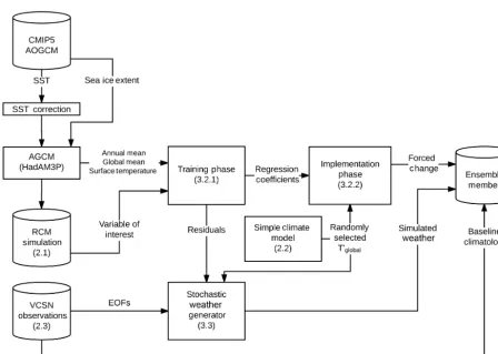
The construction of each of these signals is described in greater detail below with a high-level overview of how these contributions are related shown in Fig. 1. The methodology described below pertains to a selected single GHG emis-sions scenario and the daily maps of the climate variable of interest (X; here daily maximum (Tmax) and daily
mini-mum (Tmin) surface temperatures) are obtained from one or
more RCM simulations. To produce the results for this study, 10 ensemble members were generated for each of the 190 Tglobal time series from MAGICC to produce an ensemble
Figure 1.Flow chart illustrating the processes involved in generating a single EPIC ensemble member based on training from a selected RCM simulation. Numbers in brackets refer to the section in the text where more details are provided.
obtained from six RCM simulations driven by the Represen-tative Concentration Pathway (RCP) 8.5 GHG emissions sce-nario for the period 1971–2100. RCP 8.5 was chosen as it displays a high climate signal-to-noise ratio, resulting in the most robust regression results (Huntingford and Cox, 2000; Mitchell, 2003), but the methodology is valid for any chosen GHG emission scenario, assuming that a robust regression fit is obtained during the training phase. The assumption, which has been verified (not shown here), is that the dependence of X onTglobal is independent of the GHG emissions scenario
used for the training. All anomalies were calculated with re-spect to the period 2000 to 2010. This anomaly period was chosen because the change inXover the 21st century was of interest.
3.1 The climatology
At each 0.05◦ by 0.05◦ (approximately 5 km) grid point, a mean annual cycle is calculated from daily observational data from 2001 to 2010. For this study, these observational data were obtained from VCSN (Sect. 2.3). Since the 10-year baseline period is rather short, a climatology derived by calculating calendar day means would still contain some
weather-induced noise. Therefore, a regression model which includes an offset basis function, expanded in two Fourier se-ries (Fourier pairs) to account for seasonality (see Sect. 2.4 of Kremser et al., 2014), is fitted to the daily observational data to obtain the mean annual cycle. The first two Fourier series expansions are given by
β(d)=β0+β1×sin(2π d/365)+β2×cos(2π d/365)
+β3×sin(4π d/365)+β4×cos(4π d/365), (1)
wheredis the day number of the year andβis the regression coefficient being expanded. By using an offset basis function expanded in Fourier pairs, the resultant mean annual cycle is smooth. Examples of the mean annual cycle are shown in Fig. 2 for four selected locations around New Zealand.
5
0
5
10
15
20
25
30
35
Auckland
Wellington
2002 2004 2006 2008 2010
5
0
5
10
15
20
25
30
35
Christchurch
2002 2004 2006 2008 2010
Dunedin
Year
Surface temperature (°C)
Figure 2.Observations of daily maximum surface temperature (red) and daily minimum surface temperature (cyan) from VCSN, together with the mean annual cycle obtained from the regression model fit to the daily maximum surface temperature (magenta) and the daily minimum surface temperature (blue) time series for four selected locations in New Zealand, over the period 2001 to 2010.
3.2 Direct response toTglobal0 3.2.1 Training phase
In the training phase, the first-order long-term forced change in X is established using the correlation between X0 and Tglobal0 . This relationship is expected to be dependent on the RCM simulation from which the variable of interest is ob-tained. There are two ways in which this can be managed:
1. A statistical relationship is quantified for each RCM simulation providing data for the training phase of EPIC. Then, in the “implementation phase” of EPIC (see below), for each ensemble member, a single rela-tionship is randomly selected.
2. A single statistical relationship is quantified using a concatenated time series obtained from all RCM sim-ulations providing data for the training phase of EPIC. In the “implementation phase”, this relationship is used. For the purposes of this study, method (1) is used, as method (2) will tend to underestimate the true uncertainty of the relationship betweenX0andTglobal0 .
A simple linear correlation betweenX0andTglobal0 is cal-culated for each of the six RCM simulations and each grid
point independently, namely
X0(t )=α×Tglobal0 (y)+R(t ), (2)
whereX0(t )are the daily anomalies with respect to the 2001– 2010 mean annual cycle ofX, theTglobal0 (y)are the anoma-lies of an annual mean global mean surface temperature time series obtained from the AGCM which provided the bound-ary conditions for the selected RCM simulation,αis the re-gression coefficient, andRis the residual which is the part of the signal that cannot be explained by the statistical model. In this case, the residuals are used by the stochastic weather generator (see Sect. 3.3) to model higher-order changes in the variability inXwhich are not captured by Eq. (2).
The mean annual cycle ofX, which is used to calculate X0, is generated using the same method and time period used to calculate the mean annual cycle of the observational set. X0, rather than X, is used in Eq. (2), as the change in the seasonal cycle is of interest. Removing the mean annual cy-cle removed the need to add additional terms to describe the baseline seasonal cycle.
simula-2020 2040 2060 2080 2100 Year
4 2 0 2 4 6 8 10
Temperature anomaly [K]
HADGEM2-ES
GISS-E2-R
NORESM1-M
BCC-CSM1-1
GFDL-CM3
CESM1-CAM5
Figure 3. Annual mean global mean surface temperatures calcu-lated from the CMIP5 AOGCM simulations under the RCP8.5 sce-nario (coloured solid lines). The annual mean global means from the HadAM3P (dashed lines) and MAGICC (grey lines) for RCP8.5 are also shown.
tion. Both theTglobal0 time series used in the training phase and later in the implementation phase of EPIC need to be geophysically consistent. This geophysical consistency can be assessed by comparing the Tglobal0 time series obtained from the HadAM3P simulations with the Tglobal0 time series obtained from the CMIP5 AOGCMs that provided the SST boundary conditions for the HadAM3P simulations (which were not used elsewhere in EPIC), as well as with the 190 Tglobal0 time series obtained from MAGICC (Fig. 3). There are clear differences between theTglobal0 time series obtained from the CMIP5 AOGCMs and those obtained from the HadAM3P simulations. This is because the SSTs from the CMIP5 AOGCMs are bias-corrected before being used as the surface boundary conditions for the HadAM3P simula-tions. The six Tglobal0 time series from the HadAM3P simu-lations (used in the training phase of EPIC) fall well within the envelope of the 190 MAGICCTglobal0 time series used in the implementation phase of EPIC, even though MAGICC is emulating a range of CMIP3 models.
Because the fit coefficient,α, is expected to depend on son, it is expanded in two Fourier pairs to account for its sea-sonality (Eq. 1). The resultingαhas a smooth seasonal cycle, which would not be the case if each month was fitted inde-pendently. When embedded in Eq. (2), the resulting equation has five fit coefficients (α0toα4):
X0(t )=(α0+α1×sin(2π d/365) (3)
+α2×cos(2π d/365)+α3×sin(4π d/365)
+α4×cos(4π d/365))×Tglobal0 (y)+R(t ).
The statistical model is solved using a multivariate least squares regression approach (Moore and McCabe, 2003) to
1980 2000 2020 2040 2060 2080 2100
Year 15
10 5 0 5 10 15 20
Daily maximum surface temperature anomaly (°C)
Figure 4. An example of the fit of Eq. (2) (red line) to daily maximum surface temperature anomalies (blue) obtained from the NorESM1-M RCM simulation under the RCP8.5 GHG emissions scenario at Alexandra, New Zealand (45.249◦S, 169.396◦E). Solid line represents the zero line (no change).
obtain the fit coefficients. We refer to each such set of five fit coefficients as a tuple; recall that this fit is applied at each grid point and for each available RCM simulation.
An example of a fit of Eq. (2) to daily maximum surface temperature anomalies is shown in Fig. 4 for a location in the South Island of New Zealand.
The small annual cycle in the fit, with growing amplitude, results from summertime and wintertime daily maximum surface temperatures exhibiting different correlations against Tglobal0 . The inter-annual variation arises from changes in Tglobal as αdoes not change from year to year. In addition
to the long-term forced change, there is significant day-to-day variability. The use of the residuals from such fits in the stochastic weather generator is described in Sect. 3.3.
The unitlessαcoefficient describes a location’s sensitiv-ity to changes in annual mean global mean surface temper-ature. The magnitude of α indicates whetherTmax or Tmin
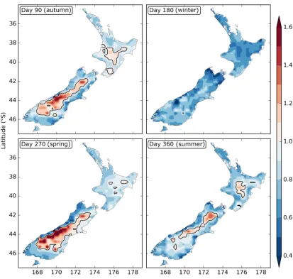
are changing faster (α >1) or slower (α <1) than the global mean surface temperature. Example maps of theα coeffi-cient, over New Zealand, for four selected days throughout the year, are shown in Fig. 5. This analysis shows that daily maximum surface temperatures over most of New Zealand are warming more slowly thanTglobal. However, high-altitude
regions, such as the Southern Alps, indicate aTmaxincreasing
faster thanTglobalfor Southern Hemisphere spring, summer,
and autumn.
Figure 5.Maps ofαcoefficients (unitless), which represent the sensitivity of changes in daily maximum surface temperature to changes in annual mean global mean surface temperatures for locations throughout New Zealand. Theαcoefficients were derived from fits of Eq. (2) to daily time series of daily maximum temperatures at each grid point of the NorESM1-M RCM simulation. The annual mean global mean surface temperature anomalies were taken from the AGCM simulation that provided the boundary conditions for this particular RCM simulation. Black lines indicateαvalues of 1.0.
refitted to obtain equally probableαfit coefficients (Bodeker and Kremser, 2015). This approach allows for the incorpo-ration of the uncertainty in the fit of Eq. (2) into the final ensemble of projections.
3.2.2 Implementation phase
Once the Monte Carlo derived sets (just one set if method (2) is used) ofαtuples have been obtained, they are used in the implementation phase of EPIC. As described in Sect. 2.2, 190 simulations of Tglobal0 can be generated using a SCM. A randomly selectedTglobal0 time series from the 190-member set is used together with a randomly selected tuple ofα val-ues to generate a series of maps of X0forced using Eq. (2),
where the forced subscript denotes that these are changes which correlate withTglobal0 .
There might be some concern that the random selection of anαtuple from the available set of tuples for a location could cause the spatial coherence in the forced signal across New Zealand to be lost, as at a nearby location a different tuple could be randomly selected. This was tested for and was found not to be the case, as the multiple instances of tuples (multiple instances of Fig. 5) are very similar and consistent (not shown here).
3.3 Indirect response toT0
re-alistic weather noise, must be present in the projections com-prising the ensemble. One potential use of the ensemble of projections generated by EPIC is assessment of the impacts and implications of climate change on a regional scale. These impacts seldom happen at a single site, i.e. the impact is felt over a large area. For this reason it is important that any spe-cific member of an ensemble is appropriately spatially co-herent over multiple sites. This is not achieved if the method considers each site in isolation, since any purely stochasti-cally determined weather noise added to a site would not be spatially coherent at neighbouring sites. For this reason, an empirical orthogonal function (EOF) approach, described by Lorenz (1956), is used to describe the spatial weather pat-terns and how they change over time. EOF analysis is a sta-tistical method which reveals the spatial patterns, or modes of variability in a data set, and how these patterns evolve over time as given by the resulting principal component (PC) time series. Hereafter we refer to these modes of variabil-ity as “weather modes”. The EOF analysis is applied toX0 after the dependence on Tglobal0 has been removed. These weather modes, and PC time series, are then used to construct a weather generator which produces realistic weather noise by stochastically generating PC time series (PCsyn). The
fol-lowing is recognised in the construction of the stochastic weather generator:
1. That VCSN data will provide the most realistic repre-sentation of weather noise.
2. That RCM simulations will simulate how that weather noise is likely to evolve in response to climate change (represented byTglobal0 ).
3. That the RCM simulations will be imperfect in simulat-ing the patterns of variability derived from the VCSN data.
4. That there will be patterns of variability (weather) whose amplitude and variability will respond to climate change as well as others which do not change with in-creases inTglobal0 .
3.3.1 Identifying the modes of variability responding to climate change
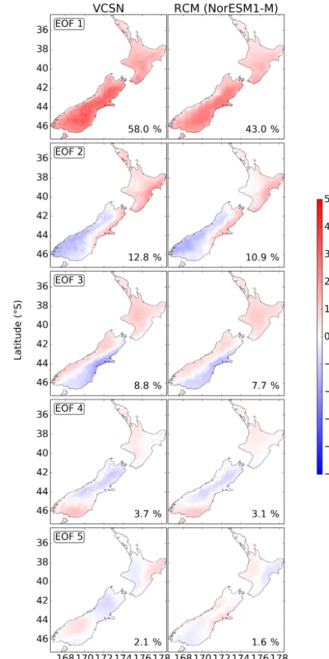
We begin by conducting an EOF analysis on VCSN data that have been detrended by removing the first-order trend and on residuals from the fit of Eq. (2) to RCM data in the train-ing phase. Where the patterns of variability obtained from EOF analyses of VCSN and RCM diverge is considered to be the cut-off point for where the RCM simulation can be taken to have any integrity with regard to simulating forced changes in weather noise. Visual inspection of the EOF maps derived from VCSN and RCM data suggested that the first four modes of variability are well represented by the RCM simulations (see Fig. 6).
Figure 6.The first five EOF patterns of weather noise in daily max-imum surface temperatures obtained from VCSN data from 1972 to 2013 (left column) and obtained from RCP8.5 NorESM1-M RCM output from 1972 to 2100. The colour bar shows the amplitude of the pattern in◦C. The percentage values in each panel show the fraction of the total variability explained by each mode.
3.3.2 Modelling forced changes in the amplitude and variability of weather modes
To compare statistics from the PC time series calculated from VCSN and RCM data, they must share the same underly-ing weather modes. This is done by projectunderly-ing the VCSN weather modes (EOFVCSN) onto the RCM data to calculate
a pseudo-PC time series. A pseudo-PC time series is lated in the same way that a standard PC time series is calcu-lated, except that the weather modes are prescribed instead of being calculated from the data. A pseudo-PC time series describes the magnitude of a particular pattern of variability from VCSN, which is present in the RCM data. The VCSN weather modes, rather than the RCM weather modes, were prescribed because the observational data set is more likely representative of patterns of variability seen in New Zealand. The pseudo-PC and VCSNPCtime series can be compared as
they both describe the same patterns of variability.
In the stochastic weather generator, we consider changes in the following two items:
1. The amplitude of the weather mode: this is quantified by correlating the associated pseudo-PC time series with Tglobal0 and then using that correlation coefficient (β) to drive a trend in the PC time series obtained from the VCSN-based EOF analysis.
2. The variability of the weather mode: this is quantified by correlating the variability in the associated pseudo-PC time series withTglobal0 and then using that correla-tion coefficient (βvar) to drive a trend in the variability of
the PC time series obtained from the VCSN-based EOF analysis. The mean variability of the weather mode is obtained from the VCSN PC time series rather than the pseudo-PC time series, so that the weather mode em-ulates the magnitude of variability seen in the VCSN data.
We also recognise that the PC time series will exhibit tem-poral auto-correlation and therefore that correlation is quan-tified and removed before correlating the PC signal, and its variability, againstTglobal0 . The resulting time series (PCsyn_n) captures both long-term shifts and/or changes in spread of thenth weather mode. We note, however, that by considering only lag-one autocorrelation in these PC time series, we ne-glect longer-term auto-correlation, e.g. that resulting from El Niño and La Niña events. As a result, our ensemble time se-ries exhibit smaller inter-annual variability than is observed in VCSN time series.
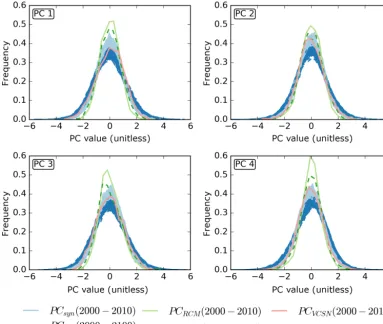
The ability of the method to generate a set of PDFs of the PCsyn_1to PCsyn_4time series is demonstrated in Fig. 7.
The EPIC method corrects for any shortcomings in the ability of the RCM to correctly simulate expected magni-tudes of weather variability for these four primary modes and then accommodates these corrections when generating PC time series that evolve into the future.
3.3.3 Modelling higher order modes of variability in weather
The stochastic weather generator includes the effects of EOF patterns five and higher but assumes that these modes show no dependence onTglobal0 as the RCM simulations do not ac-curately simulate these higher modes of weather variability. The variability of the PC time series often has a strong sea-sonal cycle. Therefore, for EOF pattern five and higher, syn-thetic PC time series (PCsyn) are generated using a standard
Monte Carlo approach, i.e. randomly selecting values from N (0, σ (d))– that is, a normal distribution with a mean of 0 and a SD which depends on the day of the year which is be-ing modelled.σ (d)is determined by a linear least squares fit of two Fourier pairs (Eq. 1) to the VCSN PC time series. The Fourier pairs model the seasonal cycle in the PC time series. This approach allows selection of extreme PC values that are outside of the range of PC values experienced in the 1972– 2013 period, but noting that the PDFs of these PCs do not evolve with time. As with the forced changes in the ampli-tude and variability of weather modes, the auto-correlation in the PC time series is also quantified and captured in the statistically modelled PC time series.
For a given ensemble member, once synthetic PC time se-ries at daily resolution have been generated, they are used to produce a reconstructed weather field,W, according to
W (i, j, t )=
50 X
n=1
EOFVCSN_n(i, j )PCsyn_n(t ),
wherei,j, andt represent the latitude, longitude, and time dimensions respectively andnis thenth weather mode.
SinceW has been constructed from a linear combination of spatial patterns of variability, each of which is spatially co-herent, it retains the property of spatial coherence. The vari-ability evolves as expected under changes inTglobal0 for the first four modes of variability, as simulated by the RCM, and where extreme conditions, outside the range of the training period, occur with a statistically reasonable frequency due to the stochasticity in the construction of the pseudo-PC time series.
Tmin is modelled identically to Tmax with one small
change: days with anomalously low Tmax would be more
likely to have anomalously lowTmin. Not accounting for this
correlation could result in stochastically modelledTmin
val-ues being higher than the modelledTmaxvalue for that day.
To avoid that, and to capture the correlation betweenTmax
andTminon any given day, the same set of random numbers
used to generate the values in the synthetic PCn time series forTmaxfor a given day is used to generate the values in the
synthetic PCn time series forTmin. This forces the selection
of PCsyn values from the same region of the PDF for both
Figure 7.PDFs of the first four synthetic (PCsyn) and RCM (PCRCM) PC time series for the first decade of the 21st century are shown as solid lines and PDFs for the last decade of the 21st century are shown as dashed lines. PCRCMand PCsynwere both derived from the NorESM1-M RCM output as an example. The PDF from the PC time series (2000–2010) obtained from VCSN is also shown (PCVCSN). The disagreement between the PCRCMand PCVCSNvalidates the use of VCSN weather noise as the basis for our stochastic weather generator, and the good agreement between the ensemble of PCsynand PCVCSNdemonstrates that the EPIC method generates synthetic PC time series with a degree of variability that matches reality.
4 Results
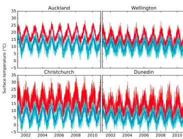
Examples of theTmaxandTmintime series generated by the
EPIC method are shown in Fig. 8 for four population cen-tres in New Zealand together with the associated VCSN time series.
Actual EPIC ensemble time series add these anomaly time series to the 2001–2010 VCSN-derived annual cycle cli-matology and therefore show no systematic bias with re-spect to the VCSN data. The EPIC-generated time series also show a long-term evolution consistent with expectations from RCM simulations, including the effects of the spread in those simulations. While it cannot be directly seen from the time series plotted in Fig. 8, the EPIC-generated time series also exhibit changes in weather variability consistent with RCM projections of expected changes in the first four modes of weather variability. The apparent annual cycle in the anomaly time series reflects the annual cycle in the vari-ance and not an annual cycle in the anomalies; towards the
end of the period there is a true annual cycle in the anoma-lies from differential seasonal changes inTmaxandTmin. The
inter-annual variability of the EPIC ensemble members is lower than that of the observational data set. This is due to EPIC not including any terms which describe patterns of variability which occur at timescales of longer than 1 year.
5 Discussion and conclusions
The EPIC (Ensemble Projections Incorporating Climate model uncertainty) method is able to generate large ensem-bles of daily time series of daily maximum and minimum temperatures that exhibit the following characteristics:
– No bias with respect to VCSN data.
use of a wider suite of RCMs as captured by the use of projections ofTglobal0 . TheTglobal0 time series were gen-erated by a SCM tuned to 19 different AOGCMs and 10 different carbon cycle models and used as a predic-tor for the long-term change inTmaxandTmin.
– Weather variability with extremes that extend beyond that observed in the VCSN record, and which evolve in a way consistent with RCM projections of changes in the four primary modes of weather variability.
– Spatial coherence in weather variability in any single ensemble member is preserved.
As such, EPIC-generated projections are suitable for gener-ating robust PDFs of projections ofTmaxandTmin.
The number of members in each ensemble is essentially limited only by the computing resources available. The stochasticity introduced by the Monte Carlo analysis and modelling of the weather noise allows for many ensemble members to be generated for a givenTglobal. For calculating
the PDFs that are delivered to users, we currently generate 19 000 member ensembles (10 ensemble members for each Tglobal) for a given RCP scenario at each 0.05◦×0.05◦grid
point across New Zealand.
A web-based tool has been developed to deliver PDFs of TmaxandTminfor the periods 2001–2010 and 2091–2100 to
users along with statistics regarding the change in frequency of extreme events, i.e. days per year withTmaxabove 25 and
30◦C and Tmin below 0 and 2◦C. The tool is available at
http://futureextremes.ccii.org.nz/.
The next steps for the development of EPIC include ex-tending the range of climate variables to daily surface broad-band radiation, surface humidity, and precipitation, and in-corporating longer-term sources of variability, e.g. those gen-erated by El Niño and La Niña events, into the stochastic weather model. The implementation of a model weighting scheme, such as that of Knutti et al. (2017), for the training data could increase the applicability of the model.
Code and data availability. The source code and data used are available upon request to the corresponding author. The VCSN data set employed is available from NIWA (2017) (https://www.niwa.co. nz/climate/our-services/virtual-climate-stations).
Competing interests. The authors declare that they have no conflict of interest.
Acknowledgements. This research was funded by the Ministry of Business, Innovation and Employment as part of the Cli-mate Changes, Impacts and Implications programme (contract C01X1225). We would also like to thank Malte Meinshausen for providing the tuning files used to emulate various AOGCMs using MAGICC, and Abha Sood for assistance with the RCM data.
Edited by: Volker Grewe
Reviewed by: two anonymous referees
References
Ackerley, D., Dean, S., Sood, A., and Mullan, A. B.: Regional cli-mate modeling in NZ: comparison to gridded and satellite obser-vations, Wea. Clim., 32, 3–22, 2012.
Bhaskaran, B., Mullan, A. B., and Renwick, J.: Modelling of atmo-spheric variation at NIWA, Wea. Clim., 19, 23–36, 1999. Bhaskaran, B., Renwick, J., and Mullan, A. B.: On application of
the Unified Model to produce finer scale climate information, Wea. Clim., 22, 19–27, 2002.
Bodeker, G. E. and Kremser, S.: Techniques for analyses of trends in GRUAN data, Atmos. Meas. Tech., 8, 1673–1684, https://doi.org/10.5194/amt-8-1673-2015, 2015.
Drost, F., Renwick, J., Bhaskaran, B., Oliver, H., and MacGre-gor, J. L.: Simulation of New Zealand’s climate using a high-resolution nested regional climate model, Int. J. Climatol., 27, 1153–1169, 2007.
Efron, B., and Tibshirani, R. J.: An Introduction to the Bootstrap, Chapman & Hall CRC Monographs on Statistics & Applied Probability, Taylor & Francis, Boca Raton, FL, USA, 1994. Friedlingstein, P., Cox, P., Betts, R., Bopp, L., von Bloh, W.,
Brovkin, V., Cadule, P., Doney, S., Eby, M., Fung, I., Bala, G., John, J., Jones, C., Joos, F., Kato, T., Kawamiya, M., Knorr, W., Lindsay, K., Matthews, H. D., Raddatz, T., Rayner, P., Reick, C., Roeckner, E., Schnitzler, K.-G., Schnur, R., Strassmann, K., Weaver, A. J., Yoshikawa, C., and Zeng, N.: Climate–carbon cy-cle feedback analysis: results from the C4MIP Model intercom-parison, J. Climate, 19, 3337–3353, 2006.
Gordon, C., Cooper, C., Senior, C. A., Banks, H., Gregory, J. M., Johns, T. C, Mitchell, J. F. B., and Woods, R. A.: The simulation of SST, sea ice extents and ocean heat transports in a version of Hadley Centre coupled model without flux adjustments, Clim. Dynam., 16, 147–168, 2000.
Gregory, D., Smith, R. N. B., and Cox, P. M.: Canopy, surface and soil hydrology, version 3, Unified model documentation Pa-per 25, UK Met Office, Berkshire, UK, 1994.
Harris, G. R., Collins, M., Sexton, D. M. H., Murphy, J. M., and Booth, B. B. B.: Probabilistic projections for 21st century Eu-ropean climate, Nat. Hazards Earth Syst. Sci., 10, 2009–2020, https://doi.org/10.5194/nhess-10-2009-2010, 2010.
Huntingford, C. and Cox, P.: An analogue model to derive addi-tional climate change scenarios from existing GCM simulations, Clim. Dynam., 16, 575–586, 2000.
Jones, R., Noguer, M., Hassell, D. C., Hudson, D., Wilson, S. S., Jenkins, G. J., and Mitchell, J. F. B.: Generating high resolu-tion climate change scenarios using PRECIS, Tech. rep., Met Oce Hadley Centre, Exeter, UK, 40 pp., 2004.
Knutti, R., Masson, D., and Gettelman, A.: Climate model geneal-ogy: Generation CMIP5 and how we got there, Geophys. Res. Lett., 40, 1194–1199, https://doi.org/10.1002/grl.50256, 2013. Knutti, R., Sedláèek, J., Sanderson, B. M., Lorenz, R.,
interdependence, Geophys. Res. Lett., 44, 1909–1918, https://doi.org/10.1002/2016GL072012, 2017.
Kremser, S., Bodeker, G. E., and Lewis, J.: Methodological as-pects of a pattern-scaling approach to produce global fields of monthly means of daily maximum and minimum temperature, Geosci. Model Dev., 7, 249–266, https://doi.org/10.5194/gmd-7-249-2014, 2014.
Lorenz, E. N.: Empirical orthogonal functions and statistical weather prediction, Scientific Report No. 1, Statistical Forecast-ing Project, Massachusetts Institute of Technology, Department of Meteorology, Cambridge, MA, USA, 52 pp., 1956.
Masson, D. and Knutti, R.: Climate model genealogy, Geophys. Res. Lett., 38, L08703, https://doi.org/10.1029/2011GL046864, 2011.
Meehl, G. A., Stocker, T. F., Collins, W. D., Friedlingstein, P., Gaye, A. T., Gregory, J. M., Kitoh, A., Knutti, R., Murphy, J. M., Noda, A., Raper, S. C. B., Watterson, I. G., Weaver, A. J., and Zhao, Z.-C.: Global climate projections, in: Climate Change 2007: The Physical Science Basis, Contribution of Working Group I to the Fourth Assessment Report of the Intergovernmen-tal Panel on Climate Change, edited by: Solomon, S., Qin, D., Manning, M., Chen, Z., Marquis, M., Averyt, K. B., Tignor, M. and Miller, H. L., Cambridge University Press, Cambridge, UK and New York, NY, USA, 2007.
Meinshausen, M., Raper, S. C. B., and Wigley, T. M. L.: Em-ulating coupled atmosphere-ocean and carbon cycle models with a simpler model, MAGICC6 – Part 1: Model descrip-tion and calibradescrip-tion, Atmos. Chem. Phys., 11, 1417–1456, https://doi.org/10.5194/acp-11-1417-2011, 2011a.
Meinshausen, M., Wigley, T. M. L., and Raper, S. C. B.: Em-ulating atmosphere-ocean and carbon cycle models with a simpler model, MAGICC6 – Part 2: Applications, Atmos. Chem. Phys., 11, 1457–1471, https://doi.org/10.5194/acp-11-1457-2011, 2011b.
Mitchell, J., Johns, T., Eagles, M., Ingram, W., and Davis, R.: To-wards the construction of climate change scenarios, Climatic Change, 41, 547–581, 1999.
Mitchell, T.: Pattern scaling: an examination of the accuracy of the technique for describing future climates, Climatic Change, 60, 217–242, 2003.
Moore, D. S. and McCabe, G. P.: Introduction to the practice of Statistics, W. H. Freeman and Company, New York, 828 pp., 2003.
Mullan, B., Sood, A., and Stuart, S.: Climate Change Projections for New Zealand: Atmosphere Projections Based on Simulations from the IPCC Fifth Assessment, Technical Report, Ministry for the Environment, Wellington, New Zealand, 2016.
Murphy, J. M., Booth, B. B. B., Collins, M., Harris, G. R., Sex-ton, D. M. H., and Webb, M. J.: A methodology for proba-bilistic predictions of regional climate change from perturbed physics ensembles, Philos. T. R. Soc. A, 365, 1993–2028, https://doi.org/10.1098/rsta.2007.2077, 2007.
Murphy, J. M., Sexton, D. M. H., Jenkins, G. J., Boorman, P. M., Booth, B. B. B., Brown, C. C., Clark, R. T., Collins, M., Harris, G. R., Kendon, E. J., Betts, R. A., Brown, S. J., Howard, T. P., Humphrey, K. A., McCarthy, M. P., McDon-ald, R. E., Stephens, A., Wallace, C., Warren, R., Wilby, R., and Wood, R. A.: UK Climate Projections Science Report: Climate change projections, Met Office Hadley Centre, Exeter, UK, avail-able at: http://ukclimateprojections.metoffice.gov.uk/media.jsp? mediaid=87851&filetype=pdf, 2009.
NIWA: VCSN data set, available at: https://www.niwa.co.nz/ climate/our-services/virtual-climate-stations, last access: 17 November 2017.
Pope, V. D., Gallani, M. L., and Rowntree, P. R.: The impact of new physical parametrization in the hadley centre climate model: HadAM3, Clim. Dynam., 16, 123–146, 2000.
Pope, V. D. and Stratton, R. A.: The process governing horizontal resolution sensitivity in a climate model, Clim. Dynam., 19, 211– 236, https://doi.org/10.1007/s00382-001-0222-8, 2002. Reisinger, A., Meinshausen, M., Manning, M., and
Bodeker, G.: Uncertainties of global warming met-rics: CO2 and CH4, Geophys. Res. Lett., 37, L14707, https://doi.org/10.1029/2010GL043803, 2010.
Sexton, D. M. H., Murphy, J. M., Collins, M. and Webb, M. J.: Mul-tivariate probabilistic projections using imperfect Climate Mod-els Part I: Outline of methodology, Clim. Dynam., 38, 2513– 2542, https://doi.org/10.1007/s00382-011-1208-9, 2012. Solomon, S., Qin, D., Manning, M., Chen, Z., Marquis, M.,
Av-eryt, K. B., Tignor, M., and Miller, H. L. (Eds.): Contribution of Working Group I to the Fourth Assessment Report of the Inter-governmental Panel on Climate Change, Cambridge University Press, Cambridge, UK and New York, NY, USA, 2007. Tait, A. and Turner, R.: Generating multiyear gridded daily rainfall
over New Zealand, J. Appl. Meteorol., 44, 1315–1323, 2005. Tait, A. B.: Future projections of growing degree days and frost
in New Zealand and some implications for grape growing, Wea. Clim., 28, 17–36, 2008.