Stability analysis of a deterministic vaccination model with non-monotonic incidence rate

*_{Corresponding author}

E-mail address: [email protected] Received September 2, 2019

Available online at http://scik.org

J. Math. Comput. Sci. 10 (2020), No. 1, 51-67 https://doi.org/10.28919/jmcs/4287

ISSN: 1927-5307

STABILITY ANALYSIS OF A DETERMINISTIC VACCINATION MODEL WITH NON-MONOTONIC INCIDENCE RATE

HARISH JOSHI1,*_{, R. K. SHARMA}2_{, GEND LAL PRAJAPATI}3

1_{Department of Mathematics, Acropolis Institute of Technology and Research, Indore-453771, M.P., India} 2_{Department of Mathematics, Govt. Holkar Science College, DAVV, Indore-452001, M.P., India}

3_{Department of Computer Engineering, Institute of Engineering and Technology, DAVV, Indore-452001, M.P., India} Copyright © 2020 the author(s). This is an open access article distributed under the Creative Commons Attribution License, which permits unrestricted use, distribution, and reproduction in any medium, provided the original work is properly cited.

Abstract: In this study, a deterministic epidemic model with vaccination and non-monotonic incidence rate is considered. This model also included the effect of temporary immunity. The model shows a disease free and an endemic equilibrium. Threshold R₀(also known as basic reproduction number) is obtained, which gives the

complete dynamics of the disease. If this threshold is less than unity, the disease-free equilibrium exists and infection disappears. If it is greater than unity, the endemic equilibrium exists and infection persists. The local and global stability of disease-free and endemic equilibrium are established. Global stability of positive equilibrium is proved by using a geometric approach given by Li and Muldowney. Numerical simulations are also given to support theoretical findings.

Keywords: endemic; non-monotonic incidence; basic reproduction number; stability; equilibrium.

1.

I

Epidemic models are significant tools in analyzing the spread and control of infectious

diseases. Quarantine, treatment and vaccination are most commonly used methods to control

spread of infectious diseases. Of these, vaccination is a proven prophylactic approach and is used

in healthy individuals to prevent occurrence of infectious diseases [1, 2]. Many infectious

diseases like measles, mumps, rubella, hepatitis B, influenza are reduced to a great extent by the

use of vaccination. Several clinical results [3]have shown that the vaccination does not give

permanent resistance to the disease. Once effect of a vaccine wanes from the body, susceptibility

towards the disease increases again. Therefore, in order to prevent the infection and eradication

of the disease, the vaccination in population must reach its optimal level. A mathematical study

[4] on a model for childhood diseases with non-permanent immunity has shown that the disease

will persist in the population if the vaccination coverage level is below a definite value. An SEIV

epidemic model [5] with a nonlinear incidence and a waning preventive vaccination has

formulated and prove that there is always a backward bifurcation for increasing the rate at which

infected individuals are treated. An epidemic model [6] has included partial temporary immunity

and saturated incidence to obtain the critical vaccination coverage necessary for eradication of

the disease.

In epidemic models, incidence is the rate at which susceptible persons become infectious.

Various incidence rates have been investigated by researchers. Bilinear, nonlinear, standard,

saturated, specific nonlinear, general incidence rates are used in epidemic models and provided a

detailed analysis of the proposed models [7-12].

Motivated from the work of [6], we are proposing an epidemic model with vaccination and

non-monotonic incidence rate 2

(1 )

SI aI

 + [12]. This incidence rate increases with smallIand

decreases with largeI_{. It also measures the psychological effect from the behavioral change of}

susceptible community when infective population becomes larger. This is important because the

number of adequate contacts between infective and susceptible population decreases at high

stage of infection due to the quarantine or isolation of infectives or the protective actions taken

2.

M

M

The model is formulated as under:

2 2

(1 ) (1 )

1

1

dS SI

p A S V q I

dt aI

dE SI

E E

dt aI

dI

E I I

dt dV

pA V V q I

dt

 _{  }

 _{ }

  

  



= − − − + + − _

+ _



= − − _

+

 

= − −

  

= − − +



(1)

where S , E , I and V denotes susceptible, exposed, infectious and vaccinated persons

respectively and initial conditions are S(0),E(0),I(0),V(0) 0. The total population at time t

is given byN = S + E + I +V.

All the parameters used in model (1) are positive. The constantAis the recruitment rate of

susceptible individuals,  is the natural death rate in the population,  _{is the average number}

of contacts of a person per unit time,  is the rate at which vaccine wanes (that is, it becomes

gradually weaker),  is the rate at which infected individuals are recovered,  is the rate at

which exposed population becomes infectious, p is the fraction of Awho are vaccinated

(0 p 1), qis the fraction of recovered people who get disease acquired immunity (0 q 1)

and a is the parameter which measures the psychological effect of disease on the population

when the infective population becomes larger.

3.

E

P

B

R

N

In this section, we determine all equilibrium states of model and basic reproduction number.

SinceN = S + E + I +V , we haveN t'( )= −A N. Ast→ ,Napproaches to the carrying

capacityA . It follows that the solutions of the system (1) remains bounded in the biologically

meaningful and positively invariant region, defined by

The disease-free equilibrium of the system (1) is P0=(S0,0,0,V0)and is given by

0 0

(1 )

,

A p Ap

S   V

    

 − + 

= _{ } =

+ +

  (2)

The basic reproduction number (R0) is defined as the average number of secondary infections when one infective individual is entered into fully susceptible population [13]. It is

very useful parameter which determines whether an infection will spread through the

population or not. We obtainedR0 by next generation matrix method described in [13].

0 0

[(1 ) ]

( )( ) ( )( )( )

S A p

R    

          

− +

= =

+ + + + + (3)

Next, solving (1) for positive equilibrium, we get 0 2

0

(1 )

S

S aI

R

= + ,V pA q I

 

+ =

+ ,E I

  

+

 

= _ _ and

I is given by

a I1 2+a I2 +a3=0 (4) where, a1=a      ( + )( + )( + )

a2=      [( + )( + )( + )−{(1−q) + }] a3=      ( + )( + )( + )(1−R0)

Herea a₁, ₂0. Thus from equation (4), it is clear that

(i) If R0is less than or equal to one, then there is no positive equilibrium.

(ii) If R0 is greater than one, then there exist a unique positive (endemic) equilibrium

* ( *, *, ,* *)

P = S E I V and is given by

2 0

* *

0

(1 )

S

S aI

R

= + , *

*

pA q I

V 

 

+ =

+ ,E* I*

  

+

 

=  

  (5)

and _* [( )( )( ) {(1 ) }]

2 ( )( )( )

q D

I

a

                

− + + + − − + +

=

where, 2 2 2 0

[( )( )( ) {(1 ) }] 4 { ( )( )( )} (1 )

D=       + + + − −q  + − a       + + + −R

4.

In this section, the local stability analysis of disease-free and endemic equilibrium is

discussed. By usingS+ + + =E I V A , the original system (1) can be reduced to the following

system:

2 2

{(1 ) } ( ) {(1 ) }

1

( )

1

( )

dS A SI

p S E q I

dt aI dE SI E dt aI dI E I dt           _{ }     = − + − − + − + − − _ + _  = − + _ + _  = − + _  (7)

where, initial conditions areS(0), (0), (0) 0E I  .

Theorem 4.1. The disease-free equilibriumP0 is locally asymptotically stable when the basic

reproduction number is less than one and is unstable when it is greater than one.

Proof. The Jacobian matrix of the system (7) is

2

2 2 2

2

2 2 2

(1 )

1 ( ) (1 ) (1 )

(1 )

( )

1 (1 )

0 ( )

I S aI

aI aI q

I S aI

J aI aI  _{  }  _{ }  _{ }     − + +   − − + − − + − −      ₋  = − +  + +    _{− +}        (8)

AtP0, we have

0

0 0

( ) (1 )

0 ( )

0 ( )

S q J S             − + − − + − −     =_ − + − _  _{− +}   

The characteristic equation of this matrix is

2

0

{+(  + )}[ +(2   + + ) +(   + )( + )(1−R)] 0= (9)

in this case P0 is locally asymptotically stable. Also, two eigen values of J0 are negative and one eigen value is positive, ifR0 is greater than one. HenceP0 is unstable in this case. Theorem 4.2. If the basic reproduction number is greater than one, then the endemic

equilibrium point P* is locally asymptotically stable. Proof. AtP_*, the Jacobian matrix of system (7) is

2

2 2 2

* * *

* *

2

* * *

* 2 2 2

* *

(1 )

1 ( ) (1 ) (1 )

(1 )

( )

1 (1 )

0 ( )

I S aI

aI aI q

I S aI

J aI aI  _{  }  _{ }  _{ }     − + +   − − + − − + − −      ₋  =  − +  + +    _{− +}       

The characteristic equation of this matrix is 3 2

1 2 3 0

A A A

 +  + + = , where

* 1 2 * 3 (1 ) I A aI      = + + + + + 2 * * *

2 2 2 2

* * *

2 ( )( ) (2 )

(1 ) (1 ) (1 )

I I I

A a

aI aI aI

 

         

= + + + + + _ + + _+

+ _ + _ +





3 * 2

*

2 ( )( )( ) ( ) ( ) ( )

(1 )

I

A a I q

aI

                

= _ + + + + + + + + + + _{ +}

Also,

(

)

1 2 3 3 (2 )( )

A A −A =    + + +     + + +





2 *

* 2 2 *

*

2 ( )( ) (2 ) [2 ( )( )(2 )

(1 )

I

a I a I

aI



               

+ + + + + + + + + + + +

+

2 2 2 2 *

2 *

{7 (5 2 )( ) 6 (2 )}]

(1 ) I q aI            + + + + + + + + + − + ,

5.

G

S

A

In this section, we observe the global stability of the two equilibriaP0 andP*. To study the global stability ofP₀, we use the method given in [14]. Rewrite the system (7) as

1

2 2

( , ),

( , ), ( ,0) 0

dX

F X Z dt

dZ

F X Z F X

dt



= _

 

= =



where,X=( )S Rstands for the number of uninfected individuals and _Z=_{( , )E I} _R2

represents

the infected population (exposed and infectious both). We denote the disease-free equilibrium

byT0=(X0,0). The following conditions (M1)and (M2)are essential for global stability:

(M1) X_{0 is globally asymptotically stable for} 1( ,0)

dX

F X

dt =

(M2) F X Z₂( , )=BZ−F X Z₂( , ), whereF X Z₂( , )0, for( , )X Z ,

where, B=D F Xz 2( 0,0) represents an M-matrix (the off-diagonal elements of B are non-negative). Then the following result holds:

Lemma 5.1. If the basic reproduction number is less than one and the assumptions(M1)-(M2)

are satisfied, then the fixed point T0=(X0,0) is globally asymptotically stable. Now, we prove the following theorem:

Theorem 5.2. The disease-free equilibrium P0 is globally asymptotically stable provided that the basic reproduction number is less than one.

Proof. LetX =( )S , Z=( , )E I andT0=(X0,0), where 0

{(1 ) }

( )

A p

X  

  

− +

=

+ . Then

1 2

{(1 ) }

( , ) ( ) {(1 ) }

1

dX A p SI

F X Z S E q I

dt aI

   _{    }



− +

= = − − + − + − −

+

AtS=S0, we haveF X1( ,0)=0 and 1( ,0) {(1 ) } ( )

dX A

F X p X

dt = = −  + −  + .

0 0 2

2 2

( )

( , ) 1 ( , )

( )

0

SI

S E S I

F X Z aI BZ F X Z

I           − + −  _{    } =_{    }− + _= − − +  _{    }

where, ( ) 0

( )

S

B   

   − +   =  _{− +}   , E Z I   =  

  and

0 2

2( , ) 1

0

SI S I

F X Z aI

   ₋    =_ + _   .

In the system (7), total population is bounded by( _{1 0}) {(1 ) }

( )

A p

N  

  

− +

→

+ , that is,

1 0

, , ( )

S E I N . Since S0(N1 0) , we have

2

0 ( 1 0) (1 )

S  N  S S +aI and hence F X Z₂( , )0. Obviously, B represents an M-matrix, so conditions (M1)and (M2)hold good and by Lemma

5.1 P0 is globally asymptotically stable providedR01.

Next, we investigate the global stability ofP* by application of a geometrical approach developed in [15] (briefly explained in Appendix A).

Theorem 5.3. If basic reproduction number is greater than one, then the endemic equilibrium

*

P of the system (7) is globally stable in regionprovided  and(1−q)  _.

Proof. Theorem 4.1 shows the instability ofP₀whenR₀ 1. By means of the uniform persistence results proved in [16, 17], the instability ofP₀ assures the uniform persistence of the system whenR01. Therefore the reduced system (7) is uniformly persistent. Now, the second additive

compound matrix [2]

J of the Jacobian matrix (8) is given by

2 2

2 2 2 2 2

[2]

2 2

(1 ) (1 )

2 (1 )

1 (1 ) (1 )

2 1

0 2

1

I S aI S aI

q

aI aI aI

I J aI I aI  _{  }   _{ }        _{  } _{− − − −} − − _{− − +}   _{+ + +}      =_ − − − − − _ +    _{− − −}   ₊   

Choose the function ( , , ) diag 1,E E,

I I

P=P S E I = _ _

 . This shows that

1 _{diag 1,}I_,I

E E

P− = _ _

Also we have _f diag 0,E I' ₂EI',E I' ₂EI'

I I

P = _ − − _

 . So that

1 _0, ' '_, ' '

f

E I E I

E I E I

P P− =diag_ − − _

 . Then

[2]

1 1

2 2

2 2 2 2 2

2

2

(1 ) (1 )

2 (1 )

1 (1 ) (1 )

' ' 2

1

' '

0 (2 )

1 f

B P P PJ P

I S aI I S aI I

q

E

aI aI E aI

E I E I

I _aI E I

I E I

E I aI  _{  }   _{ }        _{  } − − = +  _{  −} _{ −} _  _{− + + +   − − + }     _{ +  +  + }     _{ }  = −_ + + + _+ − −   _{ + }     _{− + + + −}   ₊     

The matrix B can be expressed in block form as 11 12

21 22 B B B B B   =  

 , Where

2 2

11 2 12 2 2 2 2

(1 ) (1 )

2 , , (1 ) ,

1 (1 ) (1 )

I S aI I S aI I

B B q

E

aI aI E aI

 _{  }   _{ }    _ −  −  _ = −_ + + + _ =  − − +    + + +   _ _ _{ } and 2 21 22 2 ' ' 2 1 , 0 ,

' '

(2 )

1

T

I E I

E I

E _aI

B B

I _{I E I}

E I aI  _{   }   _{  }     − + + + + − −  _ _      +   =_{ } =_{ }   _{ } − + + + −  ₊   

Let 3

( , , )u v w R be a vector, then we define a norm in 3

R as | ( , , ) | max{| |,| |u v w = u v +|w|} and

let be the Lozinski imeasure with respect to this norm. We have( )B Sup g g{ ,_{1 2}}, where

1 1( 11) | 12|

g = B + B ,g2=1(B22) |+ B21|and |B12|,|B21| are matrix norms with respect to the 1

L

vector norm and ₁ represent the Lozinski imeasure with respect to 1

L norm [18]. Then,

g1=1(B11) |+ B12|

2 2

2 2 2 2 2

(1 ) (1 )

2 max , {(1 ) }

1 (1 ) (1 )

I S aI I S aI I I

q

E

aI aI E aI E

 _{  }   _{ }     − −  = −_ + + + _+  − − −  + + +   _ _ 2

2 2 2

(1 )

2 [when (1 ) ]

1 (1 )

I S aI I

q

aI aI E

 _{  }  _{ }

  ₋

= −_ + + + _+ − 

+ +

2 2 2

1 (1 )

I SI

aI aI E

 _{  } 

 

 −_ + + + _+

+ +

 

2 '

[from(7)] 1

E I

E _aI

  

 − − −

+

E'

E 

 −

To find 1(B22) we add the absolute value of the off-diagonal elements to the diagonal one in each column ofB22, and then take the maximum value of these two sums. Thus

g2 =1(B22) |+ B21|

max E' I' 2 ,E' I' 2 E

E I    E I      I

 

=  − − − − − − − − + +

 

E' I' 2 max( , ) E

E I       I

= − − − + − − +

E' max( , ) [from(7)]

E    

= − + − −

E' [when σ > θ]

E 

 −

Therefore, ( )B Sup g g{ ,_{1 2}} E'

E

  = −. Integrating both sides at the same time, we get

0

1 1 ( )

( ) log (0)

t E t

B ds

t



this shows that

0

0 0

1

limsupsup t ( ( ( , ))) 0

t _x

q B x s x ds

t  

→ _

=

_

6.

N

S

C

R

In this paper, a vaccination model with non-monotonic incidence rate and partial temporary

(3) we obtain the threshold value of vaccinationp=(  + )[ A−     ( + )( + )] A. If this

thresholdp is less thanp, R01 and if it is greater thanp, R0 1. Thus the disease can be eradicated if the vaccinated number (p) is greater than the threshold vaccination coverage (p);

otherwise the disease will persist in the population.

Now, we provide some numerical simulations by using MATLAB in support of the

analytical findings of previous sections.

(i) Considering the parameters in system (1) asA=4,=0.1, a=2,  =0.2,  =0.2,  =0.1_,

0.01

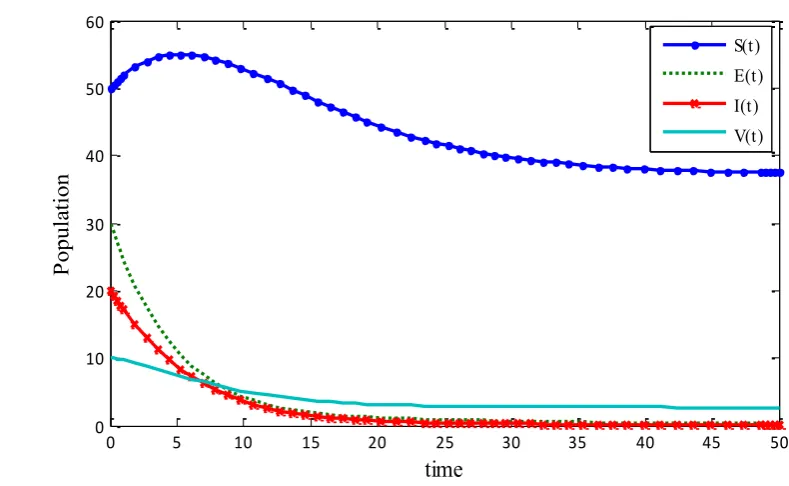
= , q=0.5and p=0.2, we get basic reproduction numberR₀=0.622 1 . Thus the system

(1) has a disease-free equilibrium P0 = (S E I V0, 0, 0, 0) = (37.2,0,0, 2.67) and is globally asymptotically stable. In this case the disease disappears and dies out (figure. 1).

(ii) Considering the parameters in system (1) asA=4,=0.2,a=2, =0.2,=0.1, =0.2,

0.2

 = ,q=0.5andp=0.2, we get basic reproduction numberR0 =4.3333 1 . Thus the system (1)

has an endemic equilibrium P*= (S E I V*, *, ,* *)=(13.6688, 2.1987,1.0994,,3.03312)and is globally asymptotically stable. Thus the disease becomes endemic and persists in the population (figure.

2).

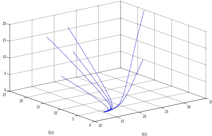
Keeping all parameters fixed of endemic equilibrium and taking different initial conditions in

system (7), the phase portrait in SEI-space is displayed. This phase diagram shows that

lim( ( ), ( ), ( ))

t→ S t E t I t = (S E I*, *, )* for R0=4.3333 1 (figure. 3).

(iii) Taking all parameters of endemic equilibrium and varying the values ofp, we see that

increase in the values ofpdecreases the infected population. At (p=0, =0), that is, without

vaccination, the size of infected population is high. At (p=0.2,=0.1) and ( p=0.4,=0.1),

that is, increasing the vaccination coverage, the size of infected population get decreases. This

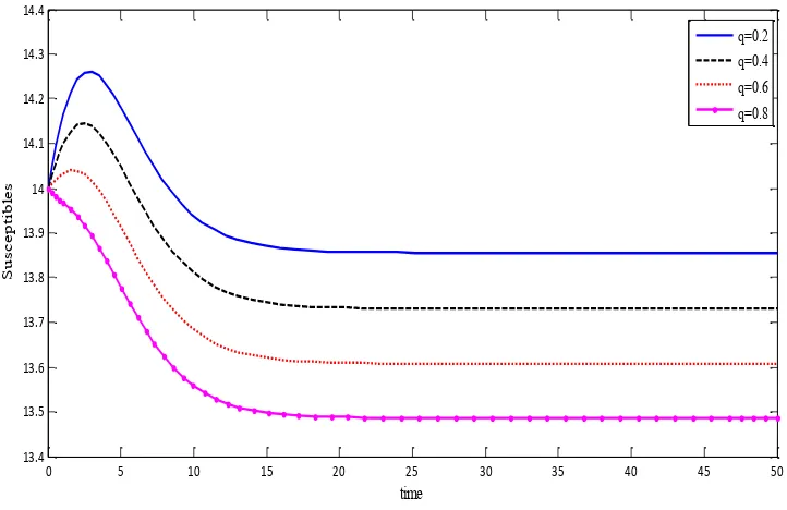
(iv) Though the basic reproduction number R0does not depend on q , numerical results show that when the disease is endemic, the steady-state value S*of the susceptible population decreases as qincreases. This indicates that qaffects the dynamics of the given system (figure.

5).

(v) On keeping all parameters fixed of endemic equilibrium and changing the values of a, we

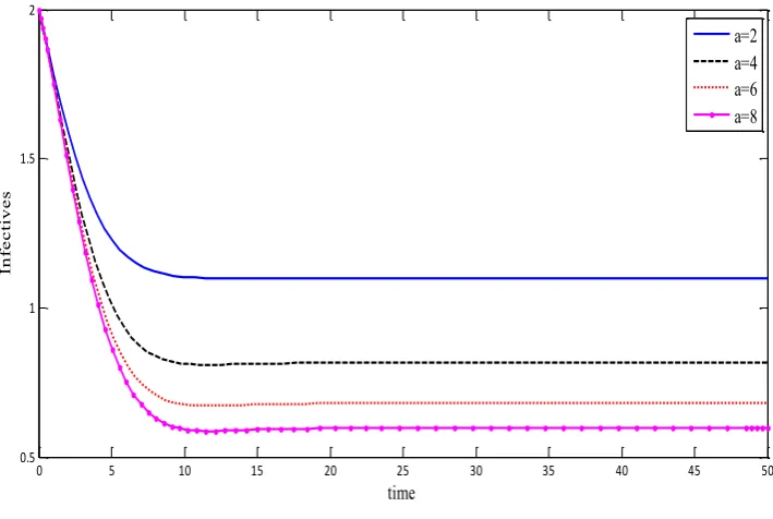
see that the steady-state values of I_*of the infectives decreases as aincreases. Thus, spread of disease decreases as the protective measures for the susceptibles increases (figure. 6).

Figure. 1. Disease-free equilibrium P₀ is globally asymptotically stable and disease dies out.

0 5 10 15 20 25 30 35 40 45 50

0 10 20 30 40 50 60

time

P

opul

at

ion

Figure. 2. Endemic equilibrium P* is globally asymptotically stable and disease persists.

Figure. 3. Phase portrait in SEI-space for endemic equilibrium.

0 5 10 15 20 25 30 35 40 45 50

0 5 10 15 20 25 30 35 40 45 50

time

P

o

p

u

la

ti

o

n

S(t) E(t) I(t) V(t)

10

15

20

25

30

35

0 5 10 15 20 25

0 5 10 15 20

S(t) E(t)

I(

Figure. 4. Effect of vaccination coverage on size of infected population.

Figure. 5. Effect of q on the size of the susceptible population.

0 5 10 15 20 25 30 35 40 45 50

0.8 1 1.2 1.4 1.6 1.8 2

time

In

fe

c

ti

v

e

s

p=0, =0 (without vaccination) p=0.2, =0.1 (with vaccination) p=0.4, =0.1 (with increased vaccination)

0 5 10 15 20 25 30 35 40 45 50

13.4 13.5 13.6 13.7 13.8 13.9 14 14.1 14.2 14.3 14.4

time

S

u

sc

e

p

ti

b

le

s

Figure. 6. The steady-state values of I* decreases as aincreases. CONFLICT OF INTERESTS

The authors declare that there is no conflict of interests.

APPENDIX A

To prove the global stability of endemic equilibrium, we briefly explain the geometrical

approach method given by Li and Muldowney [15]. Consider the system:

x = f x( ) (10)

where, _{x f x}( )_Rn

is a 1

C function about xin 1

n

D R . Let x t x( , 0)be the solution of (10) such that x(0,x₀)=x₀ and _x* _{be an equilibrium of (10), i.e.} *

( ) 0

f x = . Assume that the

following hypotheses hold:

(M3) There is a compact absorbing setKD₁.

(M4) Differential equation (10) has a unique equilibrium x* inD1.

Letx→P x( ) be a

2 2

n n

        

    matrix-valued function that is

1

C forxD₁. Suppose 1

( )

P− x exists

0 5 10 15 20 25 30 35 40 45 50

0.5 1 1.5 2

time

In

fe

c

ti

v

e

s

and is continuous forxK, the compact absorbing set. We define a quantity q as

0 0

1

limsupsup t ( ( ( , )))

t _{x K}

q B x s x ds

t 

→ _

=



where 1 [2] 1

f

B=P P− +PJ P− , the matrix P_f is obtained by substituting each elementP_ij of Pby

its derivative in the direction of f and [2]

J represents the second additive compound matrix of

the Jacobian matrixJ . The quantity ( )B is the Lozinski imeasure of B with respect to a

vector norm |.| in N

R ,

2

n N=   

 , given by 0

1 ( ) lim

h

I hB

B

h

 ₊

→

+ −

= .

The following global stability analysis result is proved in Theorem 3.5 of [15].

Theorem. Suppose that D1 is simply connected and that assumptions (M3)-(M4)hold, then the

unique equilibrium *

x of (10) is stable inD1ifq0.

CONFLICT OF INTERESTS

The authors declare that there is no conflict of interests.

REFERENCES

[1] Greenhalgh, D., Analysis threshold and stability results on age-structured epidemic model with vaccination, Theor. Popul. Boil., 33 (1988), 266-290.

[2] Liu, H., Xu, H., Yu, J., Zhu, G., Stability on coupling SIR epidemic model with vaccination, J. Appl. Math., 4 (2005), 301-319.

[3] Teitelbaulm, M.A., Edmunds, M., Immunization and vaccine-preventable illness, United States, 1992-1997, Stat. Bull. Metrop. Insur. Co., 80(2) (1999), 13-20.

[4] Moghadas, S.M., Gumel, A.B., A mathematical study of a model for childhood diseases with non-permanent immunity, J. Comput. Appl. Math., 157(2) (2003), 347-363.

[6] Sahu, G.P., Dhar, J., Analysis of an SVEIS epidemic model with partial temporary immunity and saturation incidence rate, Appl. Math. Model, 36 (2012), 908-923.

[7] Alexander, M. E., Moghadas, S. M., Periodicity in an epidemic model with a generalized non- linear incidence, Math. Biosci., 189 (2004), 75-96.

[8] Anderson, R.M., May, R.M., Regulation and stability of host-parasite population interactions, I. Regulatory processes, J. Animal Ecol., 47(1) (1978), 219-247.

[9] Capasso, V., Serio, G., A generalization of the Kermack–Mckendrick deterministic epidemic model, Math. Biosci., 42 (1978), 43–61.

[10] Gao, S., Chen, L., Nieto, J., Torres, A., Analysis of a delayed epidemic model with pulse vaccination and saturated incidence rate, Vaccine, 24 (2006), 6037-6045.

[11] Ruan, S., Wang, W.D., Dynamical behavior of an epidemic model with a nonlinear incidence rate, J. Differ. Equ., 188 (2003), 135–163.

[12] Xiao, D., Ruan, S., Global analysis of an epidemic model with non monotone incidence rate, Math. Biosci., 208 (2007), 419-429.

[13] Van den Driessche, P., Watmough J., Mathematical Epidemiology, Springer Verlag (2008).

[14] Castillo-Chavez, C., Feng, Z., Huang, W., Mathematical approaches for emerging and re-emerging infectious diseases, An Introduction, Springer Verlag (2002).

[15] Li, M.Y., Muldowney, J. S., A geometric approach to global-stability problems, SIAM J. Math. Anal., 27(4) (1996), 1070-1083.

[16] Freedman, H.I., Ruan, S., Tang, M., Uniform persistence and flows near a closed positively invariant set, J. Dyn. Differ. Eqn., 6(4) (1994), 583-600.

[17] Hutson, V., Schmitt, K., Permanence and the dynamics of biological systems, Math. Biosci., 111 (1992), 1-71. [18] Martin, R.H., Logarithmic norms and projections applied to linear differential systems, J. Math Anal. Appl.