* Corresponding author. Tel:+213-73996958 E-mail: [email protected] (B. Lakhdar)
© 2014 Growing Science Ltd. All rights reserved. doi: 10.5267/j.ijiec.2014.10.003
International Journal of Industrial Engineering Computations 6 (2015) 267–284
Contents lists available at GrowingScience
International Journal of Industrial Engineering Computations
homepage: www.GrowingScience.com/ijiec
On the application of response surface methodology for predicting and optimizing surface roughness and cutting forces in hard turning by PVD coated insert
Hessainia Zahiaa, Yallese Mohamed Athmanea, Bouzid Lakhdara* and Mabrouki Tarekb
aMechanics and Structures Research Laboratory (LMS), 8 May 1945 University of Guelma, P.O. Box 401, 24000, Algeria bUniversité de Tunis El Manar, Ecole Nationale d'Ingénieurs de Tunis (ENIT), 1002, Tunis, Tunisie
C H R O N I C L E A B S T R A C T
Article history: Received August 3 2014 Received in Revised Format October 23 2014
Accepted October 23 2014 Available online October 24 2014
This paper focuses on the exploitation of the response surface methodology (RSM) to determine optimum cutting conditions leading to minimum surface roughness and cutting force components. The technique of RSM helps to create an efficient statistical model for studying the evolution of surface roughness and cutting forces according to cutting parameters: cutting speed, feed rate and depth of cut. For this purpose, turning tests of hardened steel alloy (AISI 4140) (56 HRC) were carried out using PVD – coated ceramic insert under different cutting conditions. The equations of surface roughness and cutting forces were achieved by using the experimental data and the technique of the analysis of variance (ANOVA). The obtained results are presented in terms of mean values and confidence levels. It is shown that feed rate and depth of cut are the most influential factors on surface roughness and cutting forces, respectively. In addition, it is underlined that the surface roughness is mainly related to the cutting speed, whereas depth of cut has the greatest effect on the evolution of cutting forces. The optimal machining parameters obtained in this study represent reductions about 6.88%, 3.65%, 19.05% in cutting force components (Fa, Fr, Ft), respectively. The latters are compared with the results of initial cutting parameters for machining AISI 4140 steel in the hard turning process.
© 2015 Growing Science Ltd. All rights reserved
Keywords: Hardened steel Surface roughness Cutting forces
PVD coated ceramic tools RSM
ANOVA
Nomenclature
Vc : Cutting speed (m/min) f : Feed rate (mm/rev) ap : Depth of cut (mm)
Ra : Arithmetic average of absolute roughness (µm) Fa : Feed force (N)
Fr : Thrust force (N)
Ft : Tangential cutting force (N)
Xi : Coded machining parameters aii : Quadratic term
ANOVA : Analysis of variance
RSM : Response surface methodology DF : Degrees of freedom
Seq SS : Sequential sum of squares Adj MS : Adjusted mean squares
PC% : Percentage contribution ratio (%) R2 : Correlation coefficient
α : Clearance angle, degree γ : Rake angle, degree λ : Inclination angle, degree χr : Major cutting edge angle, degree
1. Introduction
cutting force, chip morphology and cutting temperature have not been considered for study and which are essential for hard turning study. Luo et al. (1999) have investigated the relationship between hardness and cutting forces during turning AISI 4340 steel hardened from 29 to 57 HRC using mixed alumina tools. The results suggest that an increase of 48% in hardness leads to an increase in cutting forces from 30% to 80%. It is reported that for work material hardness values between 30 and 50 HRC, continuous chips were formed and the cutting force components were reduced. However, when the work piece hardness increased above 50 HRC, segmented chips were observed and the cutting force showed a sudden increase. Davim and Figueira (2007) investigated the machinability of AISI D2 tool steel using experimental and statistical techniques. Hard turning operation was performed on material having hardness of 60 HRC. The tests were conducted by using cutting speed, feed rate and time as main parameters. The influence of cutting parameters on the flank wear evolution, specific cutting force and surface roughness variations on machinability evaluation in turning with ceramic tools using ANOVA was presented. Yallese et al. (2009) have experimentally investigated the behavior of CBN tools during hard turning of AISI 52 100 tempered steel. The surface quality obtained with the CBN tool was found to be significantly improved than grinding. A relationship between flank wear and surface roughness was also established based on an extensive experimental data. Neseli et al. (2011) exploited RSM to optimize the effect of tool geometry parameters on surface roughness in the case of the hard turning of AISI 1040 with P25 tool. Park (2002) observed that the radial force is the largest force component regardless the grade of the insert used, i.e. PCBN or ceramic during turning hardened steel in dry conditions. The specific cutting energy in the case of the hard turning is found to be smaller than in grinding. Cutting force and surface roughness were found to be smaller when cutting with PCBN tools compared to ceramic ones under similar cutting conditions. Ozel et al. (2005) conducted a set of ANOVA and performed a detailed experimental investigation on the surface roughness and cutting forces in the finish hard turning of AISI H13 steel. Their results indicated that the effects of workpiece hardness, cutting edge geometry, feed rate and cutting speed on the surface roughness are statistically significant. Davim and Figueira (2007) performed experimental investigations on AISI D2 cold work tool steel (60 HRC) using ceramic tools composed approximately of 70% AL2O3 and 30%
TiC in surface finish operations. A combined technique using an orthogonal array (OA) and analysis of variance (ANOVA) was employed in their study. The test results showed the possibility that to achieve surface roughness levels as low as Ra < 0, 8 μm with an appropriate choice of cutting parameters that eliminated cylindrical grinding. Sahoo and Sahoo (2011) conducted hard turning of AISI 4340 steel (47 HRC) using multilayer ZrCN coated carbide insert and developed mathematical model for surface roughness and flank wear. The optimized process parameter for multiple performance characteristics has been obtained using grey based Taguchi method. Mathematical model output concluded that the RSM models proposed are statistically significant and adequate because of their R2 value. Lima et al.
of AISI 4340 hardened steel using CBN-TiN-coated carbide inserts. In addition, machining cost analysis was also performed in economic conditions to compare CBN-TiN-coated and PCBN inserts. Aneiro et al. (2008) have studied the turning of hardened steel using TiCN/Al2O3/TiN coated carbide
tool and PCBN tools during turning of hardened steel. They observed that high tool life could be achieved using PCBN tool, but their cost is twice the coated carbide one. Machining medium hardened steels with TiCN/Al2O3/TiN inserts tend to be more productive. The relatively good performance of coated carbide tools in machining hardened steel relied on the coating combination of layers. Chou et al. (2002), Thiele et al. (2000) and Ozel et al. (2005) explained the effects of various factors affecting cutting forces, surface roughness, tool wear and surface integrity in hard turning of various grades of steels using CBN tools. Chou and song (2004) concluded that better surface finish could be achieved using a large tool nose radius on finish turning of AISI 52 100 bearing steel using alumina titanium-carbide tools but generates deeper white layers. Benga and Abrao (2003) and Kumar et al. (2003) observed superior surface quality in turning of hardened steel components using alumina TiC ceramic tools. In this global framework, the aim of the present study is to optimize and predicted surface roughness and cutting force components in the case of the hard turning by PVD coated ceramic insert of AISI 4140 steel alloy (56 HRC) based on statistical method. Various cutting conditions (cutting speed, feed rate, and depth of cut) were adopted for this study and response surface methodology and 33
factorial design of experiment, quadratic model have been developed with 95% confidence level.
2. Experimental procedure
2.1 Equipment and materials
The experimental work was carried out on a lathe (Tos TRENCIN; model SN 40C, spindle power 6.6 kW). The work material used during the turning tests was hardened and tempered to 56 HRC steel alloy AISI 4140 (70 mm diameter and 370 mm length). Its Chemical composition is given in Table 1. Coated ceramic insert with an ISO designation of SNGA120408T01020 (sandvik, Grade CC6050) was used in the experimental work with clamp-type PSBN25×25K12 tool holder, yielding to the following principal angle: cutting edge angle χr = 75°, negative inclination angle λ = -6°, negative rake angle γ =
-6°, clearance angle α = 6° and tool nose radius R = 0.8 mm (Sandvik , 2009).The tests were carried in dry cutting conditions.
Table1
Chemical composition of AISI 4140 steel.
Composition C Si Mn S P Ni Cu Cr V Mo Fe
% 0.42 0.025 0.08 0.018 0.013 0.021 0.022 1.08 0.004 0.209 96.95
Three levels were specified for each process parameter as given in Table 2. The factor levels were chosen within the intervals recommended by the cutting tool manufacturer (Kennametal, 2000).
Table 2
Attribution of the levels to the factors.
Level Cutting speed, Vc (m/min) Feed rate, f(mm/rev) Depth of cut, ap(mm)
1 (low) 90 0.08 0.15
2 (medium) 120 0.12 0.30
3 (high) 180 0.16 0.45
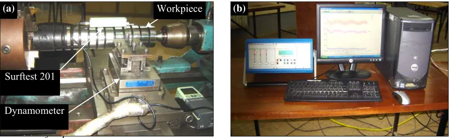
Hz was employed. The experimental setup is shown in Fig. 1;the measurements of arithmetic surface roughness (Ra) for each cutting condition were obtained from a Surftest 201 Mitutoyo roughnessmeter with a cut-off length of 0.8 mm and sampling length of 5 mm. The measurements were repeated at three equally spaced locations around the circumference of the workpiece and the result is an average of these values for a given machining pass.
2.2. Plan of experiments
For the elaboration of experiments plan the method of Taguchi for three factors at three levels was used by levels the values taken by the factors were averaged. Table 2indicates the factors to be studied and the assignment of the corresponding levels. The array chosen was the L27 (313) which have 27 rows
corresponding to the number of tests (26 degrees of freedom) with 13 columns at three levels as shown in Table 3 (Ross, 1988).The factors and the interactions are assigned to the columns.
Table 3
Orthogonal arrayL27 (313) of Taguchi (33).
L27(313) 1 2 3 4 5 6 7 8 9 10 11 12 13
1 1 1 1 1 1 1 1 1 1 1 1 1 1
2 1 1 1 1 2 2 2 2 2 2 2 2 2
3 1 1 1 1 3 3 3 3 3 3 3 3 3
4 1 2 2 2 1 1 1 2 2 2 3 3 3
5 1 2 2 2 2 2 2 3 3 3 1 1 1
6 1 2 2 2 3 3 3 1 1 1 2 2 2
7 1 3 3 3 1 1 1 3 3 3 2 2 2
8 1 3 3 3 2 2 2 1 1 1 3 3 3
9 1 3 3 3 3 3 3 2 2 2 1 1 1
10 2 1 2 3 1 2 3 1 2 3 1 2 3
11 2 1 2 3 2 3 1 2 3 1 2 3 1
12 2 1 2 3 3 1 2 3 1 2 3 1 2
13 2 2 3 1 1 2 3 2 3 1 3 1 2
14 2 2 3 1 2 3 1 3 1 2 1 2 3
15 2 2 3 1 3 1 2 1 2 3 2 3 1
16 2 3 1 2 1 2 3 3 1 2 2 3 1
17 2 3 1 2 2 3 1 1 2 3 3 1 2
18 2 3 1 2 3 1 2 2 3 1 1 2 3
19 3 1 3 2 1 3 2 1 3 2 1 3 2
20 3 1 3 2 2 1 3 2 1 3 2 1 3
21 3 1 3 2 3 2 1 3 2 1 3 2 1
22 3 2 1 3 1 3 2 2 1 3 3 2 1
23 3 2 1 3 2 1 3 3 2 1 1 3 2
24 3 2 1 3 3 2 1 1 3 2 2 1 3
25 3 3 2 1 1 3 2 3 2 1 2 1 3
26 3 3 2 1 2 1 3 1 3 2 3 2 1
27 3 3 2 1 3 2 1 2 1 3 1 3 2
The plan of experiments is made of 27 tests (array rows) in which the first column was assigned to the cutting speed (Vc), the second column to the feed rate (f), the fifth column to the depth of cut (ap) and the remaining columns to the interactions. A randomized schedule of runs was created using the design
(b)
(a) Workpiece
Dynamometer Surftest 201
Fig.1. (a) Experimental setup with measurement of the cutting forces by piezoelectric dynamometer
of experiment shown in Table 4. The response surface methodology (RSM) is a procedure for determining the relationship between the independent process parameters with the desired response and exploring the effect of these parameters on responses, including six steps (Gained et al., 2009). The latters, help to (1) define the independent input variables and the desired responses with the design constants, (2) adopt an experimental design plan, (3) perform regression analysis with the quadratic model of RSM, (4) calculate the statistical analysis of variance (ANOVA) for the independent input variables in order to find which parameter significantly affects the desired response, then, (5) determine the situation of the quadratic model of RSM and decide whether the model of RSM needs screening variables or not and finally, (6) optimize and conduct confirmation experiment and verify the predicted performance characteristics.
Table 4
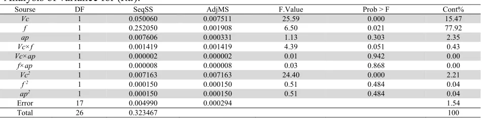
Design layout and experimental results.
Run Coded factors Actual factors Response variables
X1 X2 X3 Vc,(m/min) f,(mm/rev) ap,(mm)[m Ra,(µm) Fa,(N) Fr,(N) Ft,(N)
1 -1 -1 1 90 0.08 0.45 0.35 134.47 223.2 169.8
2 1 0 1 180 0.12 0.45 0.38 110.91 179.04 137.45
3 1 0 0 90 0.12 0.30 0.46 89.39 197.95 139.90
4 -1 0 -1 90 0.12 0.15 0.44 36.46 140.86 73.87
5 -1 -1 -1 90 0.08 0.15 0.32 34 130.08 64.14
6 1 1 0 180 0.16 0.30 0.47 72.02 206.47 143.52
7 1 -1 0 180 0.08 0.30 0.24 59.43 153.16 88.06
8 0 -1 0 120 0.08 0.30 0.31 70.02 174.88 118.39
9 -1 1 1 90 0.16 0.45 0.63 146.38 278.41 219.13
10 0 -1 1 120 0.08 0.45 0.32 110.01 203.18 152.07
11 -1 1 -1 90 0.16 0.15 0.60 38.78 156.37 100.58
12 0 1 0 120 0.16 0.30 0.50 79.88 207.49 157.92
13 1 -1 1 180 0.08 0.45 0.26 88.8 165.58 98.15
14 1 -1 -1 180 0.08 0.15 0.23 32.08 120.97 43.03
15 1 1 -1 180 0.16 0.15 0.45 38.81 142.18 78.84
16 1 0 -1 180 0.12 0.15 0.34 31.55 120.97 41.8
17 -1 0 1 90 0.12 0.45 0.47 141.94 238.14 215.15
18 0 0 0 120 0.12 0.30 0.40 78.39 183.05 129.65
19 0 -1 -1 120 0.08 0.15 0.26 33.09 123.62 52.06
20 1 0 0 180 0.12 0.30 0.37 68.59 167.67 110.53
21 1 1 1 180 0.16 0.45 0.49 120.84 274.23 179.05
22 0 0 1 120 0.12 0.45 0.42 126.42 221.16 202.84
23 0 1 -1 120 0.16 0.15 0.47 39.68 145.37 89.49
24 -1 -1 0 90 0.08 0.30 0.34 70.5 179.65 124.31
25 0 0 -1 120 0.12 0.15 0.37 36.44 133.63 73.08
26 0 1 1 120 0.16 0.45 0.53 136.35 278.17 210.92
27 -1 1 0 90 0.16 0.30 0.62 94.07 214.85 170.44
In the current study, the relationship between (cutting speed (Vc), feed rate (f) and depth of cut (ap)) and the outputs named Y, defines machinability of AISI 4140 (56 HRC) in terms of cutting forces and surface roughness. This relationship is given by:
ij e ap f Vc F
Y = ( , , )+ (1)
where Y is the desired machinability aspect and F is a function proposed by using a non-linear quadratic mathematical model, which is suitable for studying the interaction effects of process parameters on machinability characteristics. In the present work, the RMS based second order mathematical model is given by:
j i j i ij i
i ii i i i
o a X a X a X X
a
Y = +∑ +∑ +∑3
∠
2 3
1 = 3
1
where ao is constant, ai, aii, and aij represent the coefficients of linear, quadratic and cross product
terms, respectively. Xireveals the coded variables that correspond to the studied machining parameters.
The coded variables Xi,i=1,2,3 are obtained from the following transformation equations.
Vc Vco Vc X
Δ =
1 (3)
f fo f X
2 (4)
ap apo ap X
3 (5)
where X1, X2 and X3 are the coded values of parameters Vc, f and aprespectively. Vco, fo and apo are
factorsat zero level. ΔVc, Δf and Δap are the increment values of Vc, f, and ap, respectively.
3. Analysis and the discussion of experimental results
The plan of tests was developed for assessing the influence of the cutting speed (Vc), feed rate (f) and depth of cut (ap) on both the surface roughness (Ra) and cutting force components such as feed force (Fa), thrust force (Fr) and tangential cutting force (Ft). The first phase was concerned with the ANOVA and the effect of the factors and of the interactions. The second phase allowed to obtain correlations between the process parameters (quadratic regression). Afterwards, the results were through optimized. Table 4 illustrates the experimental results for surface roughness (Ra) and feed force (Fa), thrust force (Fr) and tangential cutting force (Ft).
3.1. Analysis of variance
ANOVA technique can be useful for determining influence of any given input parameters form a series of experimental results by design of experiments for machining process and it can be used to interpret experimental data. The obtained results are analyzed by statistical analysis software (Minitab-16) which is widely used in many engineering applications. The ANOVA table consists of a sum of squares and degrees of freedom. The mean square is the ratio of sum of squares to degrees of freedom and F ratio is the mean square ratio to the mean square of the experimental error. The results of the ANOVA with the surface roughness and cutting forces are shown in Tables 5 and 6 (a, b, and c), respectively. This analysis was carried out for a significance level of α = 0.05, i. e. for a confidence level of 95% (Ross, 1988). Tables 5 and 6 (a, b, and c) show the P – values, that is, the realized significance levels, associated with the F- tests for each source of variation. The sources with the P – value less than 0.05 are considered to have a statistically significant contribution to the performance measures (Gained et al. 2009). Also the last columns of the tables show the percent contribution of each source to the total variation indicating the degree of influence on the results. The greater the percentage contribution, the higher the factor influence on the performance measures.
Table 5
Analysis of variance for (Ra).
Sourse DF SeqSS AdjMS F.Value Prob > F Cont%
Vc 1 0.050060 0.007511 25.59 0.000 15.47
f 1 0.252050 0.001908 6.50 0.021 77.92
ap 1 0.007606 0.000331 1.13 0.303 2.35
Vc×f 1 0.001419 0.001419 4.39 0.051 0.43
Vc×ap 1 0.000002 0.000002 0.01 0.942 0.00
f×ap 1 0.000008 0.000008 0.03 0.868 0.00
Vc2 1 0.007163 0.007163 24.40 0.000 2.21
f 2 1 0.000150 0.000150 0.51 0.484 0.04
ap2 1 0.000150 0.000150 0.51 0.484 0.04
Error 17 0.004990 0.000294 1.54
3.1.1. Effect of cutting parameters on surface roughness
According to Table 5, the feed rate was found to be the major factor affecting the surface roughness (77.92%), this results is in a concordance with those published in (Hessainia al. 2013), (Aslan, 2005) and (Yallese et al., 2005).The cutting speed and depth of cut factors affect the surface roughness by 15,47% and 2.35%, respectively. It can be revealed that lower surface roughness values are obtained at higher cutting speeds due to lower forces generated. At high cutting speed, an improvement in surface finish was obtained since less heat was dissipated to the workpiece. It is known that the amount of heat generation increases with increase in feed rate, because the cutting tool has to remove more volume of material from the workpiece (Davim, 2011). The plastic deformation of the work piece is proportional to the amount of heat generation in the work piece and promotes roughness on the work piece surface. Depth of cut parameter has a very less effect compared to that of the feed rate. This is due to the increased length of contact between the tool and the workpiece. This improves the conditions of heat flow from the cutting zone. Similar results were also observed by (Palanikumar, 2007). From interaction plot Fig. 2a it can be observed on the one hand for a given cutting speed, the surface roughness sharply increases with increase in feed rate. On the hand, surface roughness has a tendency to be reduced with an increase in cutting speed at constant feed rate. The minimal surface roughness results with the combination of low feed rate and high cutting speed. Fig. 2b indicates that the depth of cut is low; the surface roughness is highly sensitive to cutting speed. An increase in the latter sharply reduces the surface roughness. Nevertheless, this reduction becomes smallest with higher values of depth of cut which usually does not much influence the surface roughness. Fig. 2c indicates that for a given depth of cut, the surface roughness increases with the increase in feed rate, whereas depth of cut has less effect on surface roughness. It revealed that a combination of higher cutting speed along with lower feed rate and depth of cut is necessary for minimizing the surface roughness. An improvement of surface finish Ra of 0.23 µm was recorded at higher cutting speed of 180 m/min, feed rate of 0.08 mm/rev and depth of cut of 0.15 mm.
3.1.2. Effect of cutting parameters on cutting force components
Tables 6(a, b and c) shows the results of the ANOVA for feed force (Fa), thrust force (Fr) and tangential force (Ft). It can be found that depth of cut is the most significant cutting parameter for affecting cutting forces (Fa, Fr and Ft) (90.22%, 67.64% and 69.443%), respectively. The cutting speed affects the cutting forces (Fa, Fr and Ft) by (3.66%, 5.01%, and 10.37%), respectively. The feed rate affects the cutting forces (Fa, Fr and Ft) by (2.61%, 17.36% and 14.60%), respectively. In this study, the factors and the interactions present a statistical significance Test F > Pα = 5% except for the interaction Vc×ap and f×ap for Ra, theinteraction Vc2for Fr and effect of Vc, f, and the interaction f2
for Ft. Notice that the error associated to the Tables ANOVA for the Ra was approximately 1.54%, for the Fa was approximately 0.62%, for the Fr was approximately 2.52% and for Ft was 2.02%. The interaction [for Ra (f2, ap2, Vc×f, Vc×ap, f×ap), for Fa (Vc2, f2, ap2, Vc×f, f×ap), for Fr (Vc2, f2, ap2, Vc×f, Vc×ap) and for Ft (Vc2, f2, ap2, Vc×f, Vc×ap, f×ap )] do not present a physical significance P
Fig.2. (a) 3D surface plots for interaction effects of feed rate and cutting speed, (b) depth of cut
and cutting speed, and (c) depth of cut and feed rate on surface roughness 0,3
0,4 0,5
100 125 150 0,5
0,6
0,08 175
0,12 0,16 2
Ra
f
Vc
(a)
0,35 0,40 ,
100 125 150 0,45
0,50
0,2 175
0,3 00,4
Ra
ap
Vc
(b)
0,2 0,3 0,4
0,,08 0,12 0 4
0,5
0,2 0,16
0,3 00,4
Ra
ap
f
(percentage of contribution) < error associated. As seen from the interaction plots in Fig. 3, 4, 5, (a and b) for a given cutting speed, the feed force, thrust force and tangential force sharply increases with the increase in feed rate or depth of cut. The component forces Fa, Fr and Ft are highly sensitive to depth of cut, as shown in Fig. 3, 4, 5, (c). From the above discussions it can be manifest that the precited forces can be minimized by employing lower valuer of f and ap and with higher Vc. Also it can be underlined Fr is usually the largest force among the other ones. The tangential cutting force component Ft is the middle force and Fa is the smallest one.
Using ANOVA to make this comparison requires several assumptions to be satisfied. The assumptions underlying the analysis of variance tell the residuals are determined by evaluating the following equation (Zarepour et al., 2006).
eij = yij - ŷij (6)
Fig.3. (a) 3D surface plots for interaction effects of feed rate and cutting speed, (b) depth of cut and
cutting speed, and (c) depth of cut and feed rate on feed force 50 75 100 100 125 150 100 125 0,2 175 0,3 00,4 Fa ap Vc (b) 30 60 90 0,,08 0,12 120 0,2 0,16 0,3 00,4 Fa ap f (c) 60 70 80 100 125 150 80 90 0,08 175 0,12 0,16 2 Fa f Vc (a)
Fig.5. (a) 3D surface plots for interaction effects of feed rate and cutting speed, (b) depth of cut and
cutting speed, and (c) depth of cut and feed rate on tangential force 90 120 100 125 150 150 180 0,08 175 0,12 0,16 2 Ft f Vc (a) 50 100 150 100 125 150 150 200 0,2 175 0,3 00,4 Ft ap Vc (b) 50 100 150 0,,08 0,12 150 200 0,2 0,16 0,3 00,4 Ft ap f (c)
Fig.4. (a) 3D surface plots for interaction effects of feed rate and cutting speed, (b) depth of cut and
where eij is the residual, yij is the corresponding observation of the runs, and ŷij is the fitted value. A
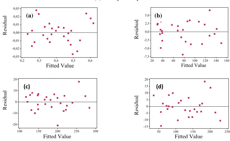
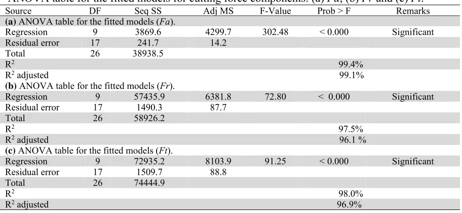
check of the normality assumption may be made by constructing the normal probability plot of the residuals. If the underlying error distribution is normal, this plot will resemble a straight line Fig.6 (a, b, c and d). Since the p-value is larger than 0.05, it is concluded that normality assumption is valid. The other two assumptions are shown valid by means of plot of residuals versus fitted values. This plot is illustrated in Fig.7 (a, b, c and d). The structure less distribution of dots above and below the abscissa (fitted values) shows that the errors are independently distributed and the variance is constant. For more information the reader can refer to the reference refer to (Montgomery & Runger, 2003).
Table 6
Analysis of variance for cutting force components: (a) Fa, (b) Fr and (c) Ft.
Sourse DF SeqSS AdjMS F.Value Prob > F Cont%
(a) Analysis of variance for (Fa).
Vc 1 1425.6 18.7 1.32 0.267 3.66
f 1 1018.7 11.9 0.84 0.373 2.61
ap 1 35132.8 339.8 23.90 0.000 90.22
Vc×f 1 13.3 13.3 0.94 0.346 0.03
Vc×ap 1 743.3 743.3 50.95 0.000 1.90
f×ap 1 227.0 227.0 15.97 0.000 0.58
Vc2 1 33.7 33.7 2.37 0.142 0.08
f 2 1 29.6 29.6 2.08 0.167 0.07
ap2 1 91.9 91.9 6.46 0.021 0.23
Error 17 214.7 14.2 0.62
Total 26 38938.5 100
(b) Analysis of variance for (Fr).
Vc 1 2957.0 72.4 0.83 0.376 5.01
f 1 10235.0 1196.0 13.64 0.002 17.36
ap 1 39861.7 493.3 5.63 0.030 67.64
Vc×f 1 445.6 445.6 4.63 0.046 0.75
Vc×ap 1 561.0 561.0 6.40 0.022 0.95
f×ap 1 2397.0 2397.0 27.34 0.000 4.06
Vc2 1 11.2 11.2 0.13 0.725 0.01
f 2 1 839.5 839.5 9.58 0.007 1.42
ap2 1 167.8 167.8 1.91 0.184 0.28
Error 17 1490.3 87.7 2.52
Total 26 58926.2 100
(c) Analysis of variance for (Ft).
Vc 1 7727 13.7 0.15 0.699 10.37
f 1 10872.7 1.4 0.02 0.900 14.60
ap 1 51699.3 2408.6 27.12 0.000 69.44
Vc×f 1 179.9 179.9 2.03 0.173 0.24
Vc×ap 1 1334.1 1334.1 14.68 0.001 1.79
f×ap 1 565.8 565.8 6.37 0.022 0.76
Vc2 1 62.4 62.4 0.70 0.414 0.08
f 2 1 1.5 1.5 0.02 0.900 0.00
ap2 1 522.5 522.5 5.88 0.027 0.70
Error 17 1509.7 88.8 2.02
Total 26 74444.9 100
3.2. Regression equations
Table 7
Table of coefficients for regression analysis, Response Ra.
Predictor Coefficient SE coefficient T Prob
Constant 0.4455 0.1116 3.99 0.00
Vc -0.00584 0.0011 -5.06 0.00
f 2.90179 1.138 2.55 0.00
ap 0.2468 0.2325 1.06 0.00
Vc2 0.0000195 0.0000 4.94 0.00
Fig.6. Normal probability plot of residuals for (a) Ra and for (b) Fa, (c) Fr and
(d) Ft respectively Residual Per cent 0,04 0,03 0,02 0,01 0,00 -0,01 -0,02 -0,03 -0,04 99 95 90 80 70 60 50 40 30 20 10 5 1 (a) Residual Pe rc en t 8 6 4 2 0 -2 -4 -6 -8 99 95 90 80 70 60 50 40 30 20 10 5 1 (b) Residual Percen t 20 10 0 -10 -20 99 95 90 80 70 60 50 40 30 20 10 5 1 (c) Residual Percen t 20 10 0 -10 -20 99 95 90 80 70 60 50 40 30 20 10 5 1 (d)
Fig.7. Plot of residuals vs. Fitted values for (a) Ra, and for (b) Fa, (c) Fr and (d) Ft,
respectively Fitted Value Re si du al 0,6 0,5 0,4 0,3 0,2 0,03 0,02 0,01 0,00 -0,01 -0,02 -0,03 (a) Fitted Value Re si du al 160 140 120 100 80 60 40 20 5,0 2,5 0,0 -2,5 -5,0 -7,5 (b) Fitted Value Res idua l 300 250 200 150 100 20 10 0 -10 -20 (c) Re si du al
Fitted Value150 200 250
The surface roughness (Ra) model is given below in Eq. (7) with a determination coefficient R2 =
98.5%; Adjusted R2 was 97.5%.
2 5 1
3 2.90 2.4 10 1.95 10 10 84 . 5 4455 .
0 Vc f ap Vc
Ra (7)
The feed force model (Fa) is given by Eq. (8) with a determination coefficient R2
of 99.4%; Adjusted R2 was 99.1 %.
Table 8
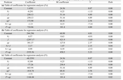
Table of coefficients for regression analysis, Response (a) Fa, (b) Fr,and (c) Ft.
Predictor Coefficient SE coefficient T Prob
(a) Table of coefficients for regression analysis (Fa)
Constant 1.6501 24.56 0.07 0.00
Vc -0.291 0.25 -1.15 0.00
f 250.13 51.16 4.89 0.00
ap 250.13 51.16 4.89 0.00
ap2 173.90 68.41 2.54 0.02
Vc×ap -1.13 0.15 -7.14 0.00
F×ap 724.86 181.4 4.00 0.00
(b) Table of coefficients for regression analysis (Fr).
Constant 244.296 60.98 4.01 0.00
Vc 0.57 0.63 -0.91 0.00
f -2297.17 621.9 -3.69 0.00
ap 301.37 127.0 2.37 0.00
Vc×f 3.17 1.47 2.15 0.04
Vc×ap 0.99 0.39 -2.53 0.02
F×ap 2355.56 450.5 5.23 0.00
(c) Table of coefficients for regression analysis (Ft).
Constant -40.5591 24.56 0.07 0.00
Vc 0.249 0.25 -1.15 0.00
f -77.26 250.4 0.91 0.00
ap 665.94 51.16 4.89 0.00
ap2 -414.74 68.41 2.54 0.02
Vc×ap -1.51 0.15 -7.14 0.00
F×ap 1144.44 181.4 4.00 0.02
1 2
1.6501- 2.91 10 228.93 250.13 173.90 -1.13 724.86
Fa Vc f ap ap Vc ap f ap (8)
The thrust force model (Fr) is given by Eq. (9) with a determination coefficient R2 of 97.5%; Adjusted
R2 was 96.1 %.
ap f ap Vc f Vc f ap f Vc Fr × 56 . 2355 + × 10 × 9 . 9 -× 17 . 3 + 06 . 7393 + 37 . 301 + 17 . 2297 -10 × 7 . 5 -296 . 244 = 1 2 1 (9)
The tangential force model (Ft) is given by Eq. (10) with a determination coefficient R2 of 98%;
Adjusted R2 was 96.9 %.
ap f ap Vc ap ap f Vc Ft × 44 . 1144 + × 51 . 1 -74 . 414 -94 . 665 + 26 . 77 -10 × 4 . 2 + 5591 . 40
= 1 2
(10)
Table 9
ANOVA table for the fitted models (Ra).
Source DF Seq SS Adj MS F-Value Prob > F Remarks
Regression 9 0.318477 0.035386 120.56 < 0.000 Significant Residual error 17 0.004990 0.000294
Total 26 0.323467
R2 98.5 % R2 adjusted 97.5 %
Table 10
ANOVA table for the fitted models for cutting force components: (a) Fa, (b) Fr and (c) Ft. Source DF Seq SS Adj MS F-Value Prob > F Remarks
(a) ANOVA table for the fitted models (Fa).
Regression 9 3869.6 4299.7 302.48 < 0.000 Significant Residual error 17 241.7 14.2
Total 26 38938.5
R2 99.4% R2 adjusted 99.1%
(b) ANOVA table for the fitted models (Fr).
Regression 9 57435.9 6381.8 72.80 < 0.000 Significant Residual error 17 1490.3 87.7
Total 26 58926.2
R2 97.5% R2 adjusted 96.1 %
(c) ANOVA table for the fitted models (Ft).
Regression 9 72935.2 8103.9 91.25 < 0.000 Significant Residual error 17 1509.7 88.8
Total 26 74444.9
R2 98.0% R2 adjusted 96.9%
Fig.8. (a) The comparison between measured and predicted value of Ra and (b), (c),
(d) comparison between measured and predicted value of Fa, Fr and Ft respectively
Surf
ace roug
hn
es
s
(µm)
Experimental Run Order
0 0,2 0,4 0,6 0,8 1
1 5 9 13 17 21 25
Ra measured Ra predicted
(a)
Feed force
(
N
)
Experimental Run Order 0
50 100 150 200 250 300 350
1 5 9 13 17 21 25 Fa measured Fa predicted (b)
Thrus
t f
orce (
N
)
0 50 100 150 200 250 300 350
1 5 9 13 17 21 25
Fr measured Fr predicted
Experimental Run Order (c)
Cutting force (
N
)
0 50 100 150 200 250 300 350
1 5 9 13 17 21 25
Ft measured Ft predicted
(d)
Analysis of variance was derived to examine the null hypothesis for regression that is presented in Tables 9-10.The result indicates that the estimated model by regression procedure is significant at α- level of 0.05.
4. Optimization of response
According to Hessainia et al. (20013), Neseli et al. (2011), one of the most important aims of experiments related to manufacturing is to achieve the desired surface roughness and cutting force components with the optimal cutting parameters. To attain this end, the exploitation of the RSM optimization seems to be a helpful technique. Here, the goal is to minimize surface roughness (Ra) and cutting forces (Fa, Fr and Ft), the parameter ranges defined for the optimization processes are summarized in Table 11.
Table11
Goals and parameter ranges for optimization of cutting conditions.
Condition Goal Lower limit Upper limit
Cutting speed, Vc is in range 90 180
Feed rate, f is in range 0.08 0.16
Depth of cut, ap is in range 0.15 0.45
Ra (µm) minimize 0.23 0.63
Fa (N) minimize 32.08 146.38
Fr (N) minimize 120.97 278.41
Ft (N) minimize 43.03 219.13
To resolve this type of parameter design problem, an objective function, F(x), is defined as follows (Myers & Montgomery, 2002):
n nj wi
i wi i d
DF 1
1
1
(11)
DF x
F( )
where di is the desirability defined for the i th targeted output and wi is the weighting of di. For various
goals of each targeted output, the desirability, di, is defined in different forms. If a goal is to reach a
specific value of Ti, the desirability di is:
0
di if i Lowi
i Low i T
i Low Yi
di if Lowi Yi Ti (12)
i High i
T
i High Yi
di if Ti Yi Highi
0
di if i Highi
For a goal to find a maximum, the desirability is shown as follows: 0
di if i Lowi
i Low i High
i Low Yi
di if Lowi Yi Highi (13)
1
di if iHighi
1
di if iLowi
i Low i High
i Y i Highi
di if Lowi Yi Highi (14)
0
di if i Highi
where the Yiis the found value of the i th output during optimization processes; the Lowiand the Highi
are, respectively, the minimum and the maximum values of the experimental data for the i th output. In Eq. (11), wi is set to one since the di is equally important in this study. The DF is a combined
desirability function (Myers & Montgomery, 2002), and the objective is to choose an optimal setting that maximizes a combined desirability function DF, i.e., minimizes F(x).
From the results shown in Fig. 9 and Table 12, it can be underlined that optimal cutting parameters found to be cutting speed (Vc) of 180m/min, feed rate (f) of 0.08mm/rev, cutting depth (ap) of 0.15mm. The optimized surface roughness Ra = 0.23µm. Also, the optimized cutting force components are: [feed force (Fa) is decreased to 29.87N with a reduction of 6.88%, thrust force (Fr) is decreased to 116.87N with a reduction of 3.65%, tangential force (Ft) is decreased to 34.83N with a reduction of 19.05%.
Table12
Response optimization for surface roughness and cutting force components.
Vc (m/min) f (mm/rev) ap (mm) Surface roughness Cutting forces
Ra, μm Fa, N Fr, N Ft, N
180 0.08 0.15 0.23 29.87 116.5 34.83
Desirability 0.99 1
Composite desirability = 0.99
Fig.9. Response optimization for surface roughness
5. Conclusions
This paper proposes the RSM approach to predicted and optimized surface roughness and cutting forces based on cutting parameters (cutting speed, feed rate and depth of cut). The important findings are summarized as follows:
1) In general, the higher is the work material hardness, the higher is the machining forces. The thrust force presents higher values followed by the tangential and feed force.
2) The machining force components increase almost linearly as the feed rate and depth of cut are elevated.
3) Feed rate and depth of cut have the greatest influence on surface roughness and cutting forces, respectively.
4) Based on the analysis of the variance (ANOVA) results, the highly effective parameters on both the surface roughness and cutting forces were determined. Namely, the feed rate parameter is the main factor that has the highest importance on the surface roughness and accounts for 77.92% contribution in the total variability of the model. The cutting speed has a secondary contribution of 15.47%, whereas the depth of cut affects fairly the surface roughness. The feed force, thrust force and cutting force are affected strongly by the depth of cut and account for 90.22%, 67.64%, 69.44% contribution in the total variability of model, respectively.
5) An improvement in surface quality and lower cutting forces are observed at higher cutting speed with lower feed rate and depth of cut.
6) Prediction accuracy of surface roughness and cutting forces by RSM developed models is efficient both for the training and testing data set.
7) The developed model has high square values of the regression coefficients which indicated high association with variances in the predictor values.
8) Comparison of experimental and predicted values of the surface roughness and cutting forces show that a good agreement has been achieved between them.
9) Response optimization show that the optimal combination of cutting parameters are found to be cutting speed of 180m/min, feed rate of 0.08mm/rev, cutting depth of 0.15mm. For machining AISI 4140 steel in the hard turning process, the optimal values of the surface roughness (Ra) = 0.23µm and cutting force components (feed, thrust and cutting forces) represent a reduction of (6.88%, 3.65% and 19.05%), respectively. These values were compared to results of initial cutting parameters.
In this study, the optimization methodology proposed is a powerful approach and can offer to scientific researchers as well industrial metalworking a helpful optimization procedure for various combinations of the workpiece and the cut material tool.
Acknowledgements
This work was achieved in the laboratories LMS (University of Guelma Algeria) in collaboration with LaMCoS (CNRS, INSA-Lyon, France). The authors would like to thank the Algerian Ministry of Higher Education and Scientific Research (MESRS) and the Delegated Ministry for Scientific Research
References
Asiltürk, I., & Akkus, H. (2011). Determining the effect of cutting parameters on surface roughness in hard turning using the Taguchi method. Measurement, 44, 1697-1704.
Aneiro, F.M., Reginaldo, T.C., & Lincoin, C.B. (2008). Turning hardened steel using coated carbide at high cutting speeds.Journal of the Brazilian Society of Mechanical Sciences and Engineering, 30, 104-109.
Aslan, E. (2005). Experimental investigation of cutting tool performance in high speed cutting of hardened X210 Cr12 cold-work tool steel (62 HRC). Materials & design, 26, 21-27.
Aouici, H., Yallese, M.A., Chaoui, K., Mabrouki, T., & Rigal, J.F. (2012). Analysis of surface roughness and cutting force components in hard turning with CBN tool: Prediction model and cutting conditions optimization. Measurement, 45, 344-353.
Benga, G.C., & Abrao, A.M. (2003). Turning of hardened 100Cr6 bearing steel with ceramic and PCBN cutting tools. Journal of Materials Processing Technology, 143-144, 237-241.
Casto, L.S., Valvo, L.E., & Ruis, V.F. (1993). Wear mechanism of ceramic tools. Wear, 160, 227-235. Chou, Y.K., Evans, C.J., & Barash, M.M. (2002). Experimental investigation on CBN turning of
hardened AISI 52 100 steel. Journal of Materials Processing Technology, 124, 274-283.
Chou, Y.K., & Song, H. (2004). Tool nose radius effects on finish turning. Journal of Materials
Processing Technology, 148, 259-268.
Davim, J.P., & Figueira, L. (2007). Comparative evaluation of conventional and wiper ceramic tools on cutting forces, surface roughness, and tool wear in hard turning AISI D2 steel. J. Engineering
Manufacture, 221, 625-633.
Davim, J.P., & Figueira, L. (2007). Machinability evaluation in hard turning of cold work tool steel (D2) with ceramic tools using statistical techniques. Materials & design, 28, 1186-1191.
Davim, J.P. (Ed). (2011). Machining of hard Materials. Springer.
Gained, V.N., Karnik, S.R., Faustino, M., & Davim, J.P. (2009). Machinability analysis in turning tungsten-copper composite for application in EDM electrodes. International Journal of Refractory
Metals and Hard Materials, 27, 754-763.
Gaitonde, V.N., Karnik, S. R., Figueira, L., & Davim, J.P. (2011). Performance comparison of conventional and wiper ceramic inserts in hard turning through artificial neural network modeling.
International Journal of Advanced Manufacturing Technology, 52, 101-114.
Gaitonde, V.N., Karnik, S. R., Figueira, L., & Davim, J.P. (2009). Analysis of machinability during hard turning of cold work tool steel (Type: AISI D2). Materials and Manufacturing Processes, 24, 1373-1382.
Hessainia, Z., Belbah, A., Yallese, M.A., Mabrouki, T., & Rigal, J.F. (2013). On the prediction of surface roughness in the hard turning based on cutting parameters and tool vibrations. Measurement, 46, 1671-1681.
Koelsch, J. (1992). Beyond TiN: New tool coatings pick up where TiN left off. Manufacturing
Engineering, 27-32.
Kumar, A.S., Durai, R., & Sornakumar, T. (2003). Machinability of hardened steel using alumina based ceramic cutting tools. International Journal of Refractory Metals and Hard Materials, 21, 109-117. Kennametal, H. (2000). Kennametal Hertel News Catalogue, News I 2000, Trade catalogue, Germany. Lalwani, D.I., Mehta, N.K., & Jain, P.K. (2008). Experimental investigations of cutting parameters
influence on cutting forces and surface roughness in finish hard turning of MDN250 steel. Journal
of materials processing technology, 206, 167-179.
Luo, S.Y., Liao, Y.S., & Tsai, Y.Y. (1999). Wear characteristics in turning high hardened alloy steel by ceramic and CBN tools. Journal of Materials Processing Technology, 88, 114-121.
Lima, J.G., Avila, R.F., Abrao, A.M., Faustino, M., & Davim, J.P. (2005). Hard turning: AISI 4340 high strength low steel and AISI D2 cold work tool steel. Journal of Materials Processing
Technology, 169, 388-395.
Montgomery, D.C. (2001). Design and analysis of experiments. John Wiley & sons, New York.
More A. S., Jiang, W., Brown, W.D., & Malshe, A.P. (2006). Tool wear and machining performance of CBN-TiN coated carbide inserts and PCBN compact inserts in turning AISI 4340 hardened steel.
Journal of Materials Processing Technology, 180, 253-262.
Montgomery, D.C., & Runger, G.C. (2003). Applied statistics and probability for engineers, third ed. John wiley & sons inc., USA
Montgomery, D.C., (2000). Design and analysis of experiments. John Wiley & sons.
Myers, R.H., & Montgomery, D.C. (2002). Response surface methodology: process and product optimization using designed experiments, 2nd ed. John Wiley and Sons, Inc.: New York,
Neseli, S., Yaldiz, S., & Türkes, E. (2011). Optimization of tool geometry parameters for turning operations based on the response surface methodology. Measurement, 44, 580-587.
Ozel, T., Hsu, T.K., & Zeren, E. (2005). Effects of cutting edge geometry, workpiece hardness, feed rate and cutting speed on surface roughness and forces in finish turning of hardened AISI H13 steel.
International Journal of Advanced Manufacturing Technology, 25, 262-9.
Ozel, T., & Karpat, Y. (2005). Predictive modelling of surface roughness and tool wear in hard turning using regression and neural Networks. International Journal of Machine Tools and Manufacture, 45, 467-479.
Park, Y.W. (2002). Tool material dependence of hard turning on the surface quality. International
Journal of the Korean Society of Precision Engineering, 3, 76-82.
Palanikumar, K. (2007). Modeling and analysis for surface roughness in machining glass fibre reinforced plastics using response surface methodology. Materials & design, 28, 2611–2618.
Ross, P. (1988). Taguchi techniques for quality engineering –loss function. Orthogonal experiments. Parameter and tolerance design, McGraw-Hill. New York, 10-50
Sahin, Y. (2003). The effect of A1203, Ti(C, N), and tin coatings on carbide tools when machining metal matrix composites. J. Surface Coatings and Technology, 24-8, 671-679.
Suresh, P.V.S., Rao, P.V., & Deshmukh, S.G. (2002). A genetic algorithmic approach for optimizing of surface roughness prediction model. International Journal of Machine Tools and Manufacture, 42, 675-680.
Sahoo, A.K., & Sahoo, B.D. (2011). Mathematical modelling and multi-response optimization using response surface methodology and grey based Taguchi method: an experimental investigation.
International journal experimental design and process optimisation, 2, 221-242.
Sandvik, C. (2009). Catalogue General, Outils de coupe Sandvik Coromant, Tournage – Fraisage – perçage – Alésage – Attachements.
Sahin, Y., & Motorcu, A.R. (2005). Surface roughness model for machining of mild steel by coated cutting tools. Materials & design, 26, 321-326.
Thiele, J.D., Roberta, A.P., Thomas, R., & Shreyes, N.M. (2000). Effect of cutting edge geometry and workpiece hardness on surface residual stresses in finish hard turning of AISI 52 100 steel. ASME
Journal of Manufacturing Science and Engineering, 122, 642-649.
Vikram K.C.H.R., Kesavan, N.P., & Ramamoorthy, B. (2008). Performance of TiCN and TiAIN tools in machining hardened steel under dry, wet and minimum fluid application.
International Journal of Machining and Machinability of Materials, 3, 133-142.
Yallese, M.A., Chaoui, K., Zeghib, N., Boulanouar, L., & Rigal, J.F. (2009). Hard machining of hardened bearing steel using cubic boron nitride tool. Journal of Materials Processing Technology, 209, 1092-1104.
Yallese, M.A., Rigal, J.F., Chaoui, K., & Boulanouar, L. (2005). The effects of cutting conditions on mixed ceramic and cubic boron nitride tool wear and on surface roughness during machining of X200Cr12 steel (60 HRC). Journal of Engineering Manufacture, 219, 35-55.