Retailer’s optimal ordering policies with cash discount and progressive payment scheme derived algebraically Pages 891-900 Download PDF

(1)

Contents lists available at GrowingScience

International Journal of Industrial Engineering Computations

homepage: www.GrowingScience.com/ijiec

Retailer’s optimal ordering policies with cash discount and progressive payment scheme derived algebraically

Alok kumara, K K Kaanodiyab, and R R Pachauric*

a_{Institute of Engineering and Technology, Khandhari, Agra, India} b_{Department of Mathematics BSA College Mathura, India}

c_{Research Scholar Dept. of Mathematics, B.S.A. College, Mathura, India}

A R T I C L E I N F O A B S T R A C T

Article history:

Received 10 September 2010 Received in revised form May, 20, 2011 Accepted 28 May 2011 Available online 31 May 2011

This study presents optimal ordering policies for retailer when supplier offers cash discount and two progressive payment schemes for paying of purchasing cost. If the retailer pays the outstanding amount before or at first trade credit period M, the supplier provides rcash discount and does not charge any interest. If the retailer pays after M but before or at the second trade period N offered by the supplier, the supplier provides r cash discount and charges interest on unpaid balance at the rate . If retailer pays the balance after N, N then the supplier does not provide any cash discount but charges interest on unpaid balance at the rate . The primary objective of this paper is to minimize the total cost of inventory system. This paper develops an algebraic approach to determine the optimal cycle time, optimal order quantity and optimal relevant cost. Numerical example are also presented to illustrate the result of propose model and solution procedure developed.

Keywords:

EOQ

Permissible delay in payments Trade credit

Cash discount Algebraic approach

1. Introduction

In classical economic order quantity model, it is tacitly assumed that the retailer must pay to the supplier for the items as soon as consignment received by him. However, this assumption may not hold in some cases. In real life situation, the supplier often offers the retailers a fixed time period to settle the account. During this period retailers can sell the items and accumulate revenue and earn interest before the end of permissible fixed period. Many researchers investigate this problem under various conditions.

(2)

892

supplier offers a permissible delay period in the paying of purchasing cost to his/her retailer and the retailer is also intern offer a permissible delay period to his/her customer to develop retailer’s replenishment policy. Recently Goyal et. al (2007) and Soni and Shah (2008) developed an inventory model in which the supplier offers two opportunity of trade credit to his/her customer with the case of constant and stock-dependent demand

A newer application of the cash discount has emerged in recent years. Some supplier are now offering instantaneous cash discount on products if the customer will pay in cash rather than using a credit card. Traditionally, the cash discount now become a marketing and customer relations strategy that is early return of invested capital which reduce credit expense, obtain faster payment of products and stimulate more sales. Many published paper related to the inventory policy under cash discount and payment delay can be found in Arcelus et al. (2001), Chang (2002), Ouyang etal. (2002), Huang and Chung (2003), Recently Ouyang et al. (2005) developed a EOQ model with deterioration items and one opportunity of cash discount. Later Chung (2008) extend Ouyang’s model in the case of deterioration rate is not sufficient small with cash discount policy. While Huang et al. (2007) developed an EPQ model with cash discount and permissible delay in payments derived algebraically.

On the other hand an algebraically technique become an easy approach to determine optimal solutions for those student who have little knowledge of calculus, may feel difficult to prove optimality condition with second order derivatives. Many research papers published on various inventory problems by applying second order derivative test to prove optimality conditions. Therefore, an algebraic approach can be also used to derive this problem. In this direction, Grubbstrom and Eedem (1999) and Cardenas-Barron (2001) showed that the formulae for the EOQ and EPQ with backlogging and shortages respectively can be derived without differential calculus. Yan and Wee (2002) developed algebraically the optimal replenishment policy for the integrated vendor-buyer inventory system without derivatives. Wu and Ouyang (2003) modified Yan and Wee (2002) in the light of shortages using algebraic method. Recently, Huang (2006) developed retailer’s replenishment policy under two levels of trade credit and limited storage space derived without derivatives.

This paper extends Goyal et al. (2007) model to allow cash discount and applying algebraic method to obtain optimal solution. As a result, our proposed research paper here is that the supplier provides not only cash discount but also permissible delay period for settlement of payment. In addition, we develop an algebraic approach to determine optimal cycle time, optimal order quantity and optimal total relevant cost under said conditions. Here the objective function is to optimize a total cost of inventory systems for the retailer. Numerical examples are illustrated to managerial insight to proposed problem with help of an algorithm.

2. Assumptions and notations

The following assumptions and notations will be used throughout:

2.1 Assumptions

1) The inventory system deals with the single item.

2) Demand rate , is known and constant.

3) Time horizon is infinite.

4) Lead-time is zero, shortages are not allowed.

5) Replenishment rate is infinite.

6) The interest charges and cash discount policies are as follows:

(3)

o If the retailer pays after the offered period , but before or at offered period , he can keep the difference in the unit sales price and unit purchase price in an interest bearing account at the rate of /unit/year. During the period , , the supplier provides r cash discount and charges interest on unpaid balance at rate . o If the retailer pays after the offered period , then the supplier does not provide any

cash discount but charges interest on unpaid balance at rate . Here the interest

rate .

2.2 Notations

1) Inventory holding cost/unit/year excluding interest charges 2) Selling price/unit

3) Unit purchase cost, with 4) Ordering cost/order 5) Replenishment cycle

6) First offered credit period in settling the account without any charges

7) Second permissible credit period in settling the account with interest charges on un-paid balance and

8) Interest earned/$/year

9) Cash discount rate offered on credit period .

10) Cash discount rate offered on credit period and . 0 1 11) Demand rate per year.

12) Order quantity, 0.

13)IHC Inventory holding cost/time unit 14)OC Ordering cost/time unit

15) Purchasing cost/time unit.

16) Interest charged per $ in stock per year by the supplier when retailer pays during , 17) Interest charged per $ in stock per year by the supplier when retailer pays during , 18) On-hand inventory at time 0 .

3. Mathematical model

The inventory level is depleted due to demand. Hence, the rate of change of inventory

, 0 1

with boundary conditions: 0 and 0. The solution of the above differential Eq. 1 is,

, 0 (2)

This at 0 gives the order quantity,

. 3

The ordering cost, inventory holding cost and purchasing cost of the system are as follow:

Annual ordering cost (OC) (4)

Annual inventory holding cost (IHC) (5)

Annual purchasing cost 1 for case

1 for case (6)

for case

Following the assumptions regarding the interest charged and interest earned, based on the length of the cycle time , three cases may arise:

(4)

894

Fig. 1. Case 1: Fig. 2. Case 2 Fig. 3.Case 3

Case 1: When (see Fig. 1)

Here, the retailer sells units during 0, and paying for units in full to the supplier at time with zero interest charged i.e.

0 (7)

During the period 0, the retailer sells units and deposits the revenue into the interest bearing account that earns ⁄$⁄ . For the period , , the retailer deposits the revenue into the account that earns /$/year. Therefore interest earned, , per year is given by

2

(8)

Using equations 4, 5, 6,7, 8 then total cost, per time unit of an inventory system:

2 1 2

(9)

Case 2. (See Fig. 2)

The retailer sells units and deposits the revenue into an interest earning account at an interest rate /$/year during 0, . Hence interest earned, during 0, is

2 .

10

Retailer purchases -units at time 0 and pays at the rate of $/unit to the supplier during 0, . The retailer sells -units at sell price $ /unit. Therefore, he has generated revenue of plus the interest earned, during 0, which arises two cases:

Sub-cases 2.1Let 1

The retailer has an adequate amount in his account to pay all -unit purchase cost at time . Therefore, retailer gets cash discount at . Then interest charges:

. 0 11

In addition, the interest earned is as follows,

. . 12

Using Eqs. (4-6), Eq. (11) and Eq.(12) the total cost, per time unit of an inventory system is given by

. . . . 1 (13)

Sub-cases 2.2Let 1

(5)

. ₂ ₂

14

and the interest earned

. 15

Using Eqs. (4-6) and Eq. (14-15) the total cost . , per time of an inventory system is given by

. . . ₂ 1 ₂ ₂

16

Case 3 (See Fig. 3)

Based on the total purchase cost, , total money in account at and total money at , three sub-cases may arise,

Sub-case 3.1. Let 1

Here retailer will pay the total purchase cost at and there is no interest charge. So, this Sub-case become the same as sub-case 2.1

Sub-case 3.2 Let 1 and

1

The retailer does not have sufficient balance to settle his/her account at time , but he/she can pay off the total purchase cost before or at . Hence retailer only pays at and the supplier start to charge the retailer the un-paid balance with interest at time . So, this sub-case becomes similar to Sub-case 2.2

Sub-case 3.3 Let 1 and

1

Here, the retailer does not have sufficient balance in his account to pay off total purchase cost at .

He will do payment of at and at . Therefore, he has to

pay interest charges on the un-paid balance 1 with interest during

, and un-paid balance 1 1 with interest

rate during , .

Therefore, total interest charges; . per time is

. ₂

= , 17

and total interest earned per time unit is

. . (18)

Using Eqs. (4-6) and Eqs. (17-18) the total cost . per time unit of an inventory system is

given by

(6)

896

. ₂ ₂ ₂ ₂

19

4. Optimal solution using algebraic method

We can rewrite

2

2 1 .

20

According to Eq. 20 the minimum of is obtained when the quadratic non-negative term, depending on , is made equal to zero. Therefore, the optimum value is

If 2 0 (21)

Therefore, Eq. 20 has a minimum value for the optimal value of reducing to

2 1 . (22)

Similarly, we can derive

. ₂ 2 2 1 . ₂₃

According to Eq. 23 the minimum of . is obtained when the quadratic non-negative term,

depending on , is equal to zero. Therefore, the optimum value . is

.

2

If 2 0

(24)

Therefore, Eq. 23 has a minimum value for the optimal value of . reducing . to

. . 2 1 . (25)

Similarly,

.

1 2

2 1 ₂

1

1 2 1

2

1 1

2

(26)

According to Eq. 26 the minimum of . is obtained when the quadratic non-negative term,

(7)

.

2 1 ₂

1

If 2 1 0. 27

. . 1 2 1 ₂

1 1 1

2

28

Similarly,

.

2

2 2 1 ₂ ₂

2 2 1

2 2

1

2

29

Eq. 29 represents that the minimum of . is obtained when the quadratic non-negative term,

depending on , is made equal to zero. Therefore, the optimum value _. is

.

2 2 1 ₂ ₂

If 2 2 1 0 30

. .

2 2 1

2 2

1

2

(8)

898

5. Algorithm

Step 1: Compute from the case 1,

Step 2: If go to step 9, otherwise, go to step 3, Step 3: If go to step 4, otherwise, go to step 8,

Step 4: If 1 go to step 6, otherwise, go to step 5,

Step 5: If 1 and 1

go to step 7, otherwise go to step 8.

Step 6: Compute . from sub-case 2.1 or sub-case 3.1 go to step 9,

Step 7: Compute _. from sub-case 2.2 or sub-case 3.2 go to step 9, Step 8: Compute . from sub-case 3.3 go to step 9,

Step 9: Compute go to step 10, Step 10: Compute min , Step 11: End.

6. Numerical example

$8, $10, .3%, .5%, .6%, .08year, .16year, 1200units/year

5/units/year.

Table 1

The optimal solution for different values of A and r

$ (Year) ($) ($)

.30 .34 .38 .0456 6870.18 6486.18 6102.18 54.72 .30 .34 .38 .0791 7190.95 6806.95 6422.95 94.92 .30 .34 .38

. .1271 . 7482.73

. 7098.73 . 6714.73 . 152.52 .30 .34 .38

. .1455 . 7592.79

. 7208.79 . 6824.79 . 174.6 .20 .24 .28 . .1599 . .1622 . .1645 . 8721.62 . 8333.87 . 7946.85 . 191.88 . 194.64 . 197.4 .20 .24 .28 . .1741 . .1766 . .1791 . 8841.39 . 8451.93 . 8063.26 . 208.92 . 211.92 . 214.92

. .2055 . 13494.2 . 246.6

. .2145 . 13589.44 . 257.4

For fixed value of and increase in cash discount rate , the cycle time and ordering quantity increase but total relevant cost decreases. As the value of increases, the cycle time, total relevant cost and ordering quantity also increase.

7. Sensitive analysis

(9)

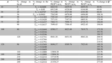
Table 2

Sensitivity analysis

% change in the

% change in the % change in

at

% change in at

% change in

10 8 0.0408 6823.92 6439.92 6055.92 48.96

12 0.05 6912.00 6528.00 6144.00 60.00

30 24 0.0707 7111.00 6727.00 6343.00 84.84

36 . 0.0903 7262.00 6878.00 6494.00 108.36

60 48 . 0.1103 7381.64 6997.64 6613.64 132.36

72 _. 0.1420 7571.91 7187.91 6803.91 170.40

75 60 . 0.1217 7482.73 7098.73 6714.73 146.04

90 . 0.1617 7690.45 7306.45 6922.45 194.04

100 80 _. 0.1444

. 0.1516

. 0.1536

8590.17 8025.00 7819.73 173.28

181.92 184.32

120 . 0.1741

. 0.1766

. 0.1791

8841.38 8451.92 8063.26 208.92 211.92 214.92

120 96 . 0.1569

. 0.1648

. 0.1669

8696.37 8309.76 7923.01 188.28

197.76 200.28

144 . 0.1888 13804.30 225.96

180 144 . 0.1888 13804.30 225.96

216 _. 0.2214 15718.96 265.68

200 160 _. 0.1961 11523.27 235.32

240 . 0.2314 21354.27 277.68

For fixed value of and increases in cash discount rate , the cycle time, and ordering quantity increase but total relevant cost decreases. As the value of increases, then cycle time, total relevant cost and ordering quantity also increase. Now in this section we study the effects of changes in the values of the system parameter , , , and on the optimal cycle time, total relevant cost and economic order quantity derived by the proposed method. The sensitive analysis is performed here by changing the value of , , , and ( $180 only for ) by 20%, 20% taking one parameter only at a time and keeping remaining other parameters unchanged.

Table 3

Sensitivity analysis of the optimal solution

Parameters % change in

the parameters % change in the

% change in at

% change in

C 6.4 0.0456 5526.18 5218.98 4911.78 54.72

9.6 0.0456 8214.18 7753.38 7292.58 54.72

P 8.0 0.0475 6911.17 6527.17 6143.17 57.00

12.0 0.0440 6828.71 6444.71 6060.71 52.80

h 4.0 0.0488 6841.88 6457.88 6073.88 58.56

6.0 0.0430 6896.76 6512.76 6128.76 51.60

M 0.064 0.0456 6927.78 6543.78 6159.78 54.72

0.096 0.0456 6812.58 6428.58 6044.58 54.72

N 0.128 0.1962 27896.85 235.44

0.192 0.2174 19756.36 260.88

When value of , , , and increases then the optimal cycle time (stable for and but decreases for and , and increases for ), total relevant cost (increases for and but decreases for

, and ) and optimal order quantity ( stable for and but decreases for and , and increases for ) for the fixed value of the parameters total relevant cost decreases.

7. Conclusions

(10)

900

credit periods and two different cash discounts on said credit periods to settlement the account of purchasing goods. By using the numerical examples, sensitive analysis is performed to study the effects of the changes of the parameter values of and , , , and on the optimal cycle time, optimal order quantity and total relevant cost respectively.

References

Aggrawal, S.P., & Jaggi, C.K. (1995). Ordering policies of deteriorating items under permissible delay in payments. Journal of the Operational Research Society 46, 658-662.

Arcelus, F. J., Shah, N.H., & Srinivasan, G. (2001). Retailer’s response to special sales: price discount vs trade credit. Omega 29, 417-428.

Cardenas-Barron, L.E. (2001). The economic production quantity (EPQ) with shortage derived algebraically.

International Journal of Production Economics, 70, 289-292.

Chand, S., & Ward, J. (1987). A note on economic order quantity under conditions of permissible delay in payments. Journal of Operational Research Society 38, 83-84.

Chang, C.T. (2002). Extended Economic Order Quantity model under cash discount and payment delay.

International Journal of Information and Management Science 13, 57-69.

Chang, K.J., & Liao, J.J. (2006). The Optimal Ordering policy in a DCF analysis for deteriorating Items when trade credit depends on the order quantity. Journal of Production Economics100, 116-130.

Chung, K.J. (2000). The inventory replenishment policy for deteriorating items under permissible delay in payments Opsearch, 37, 267-281.

Goyal, S.K., Teng, J.T., & Chang, C.T. (2007). Optimal ordering policies when supplier provides a progressive interest scheme. European Journal of Operational Research 179,404-413.

Grubbstrom, R.W., & Erdem, A. (1999). The EOQ with backlogging derived without derivatives,

InternationalJournal of Production Economics, 59, 529-530.

Huang, Y,F., & Chung K.J. (2003). Optimal replenishment policies in the EOQ model under cash discount and trade credit, Asia-Pacific Journal of Operational Research. 20, 177-190.

Huang, Y.F. (2006). An inventory model under two levels of trade credit and limited storage space derived without derivatives. Applied Mathematical Modelling 30, 418-436.

Huang, Y.F. (2007). Economic order quantity under conditionally permissible delay in Payments. European Journal of Operational Research 176, 911-924.

Huang, Y.F., Chou, C.L. & Liao, J.J. (2007). An EPQ Model under cash discount and permissible delay in payments derived without derivatives. Yugoslav Journal of Operations Research, 17, (2), 177-193.

Jamal, A.M.M., Sarker, B.R. & Wang, S. (1997). An ordering policy for deteriorating items with allowable shortage and permissible delay in payment. Journal of Operational Research Society, 48, 826-833.

Liao, H.C., Tsai C.H. & Su, C.T. (2000). An inventory model with deteriorating items under Inflation when a delay in payment permissible. International Journal of Production Economics 63, 207-214.

Mondal, B.N., & Phaujdar, S. (1989c). Some EOQ models under permissible delay in payments. International

Journal of Management Science 5, 99-108.

Ouyang, L.Y., Chang, C.T., & Teng, J.T. (2005). An EOQ model for deteriorating items under Trade credits, Journal of Operational Research Society, 56, 719-726.

Ouyang, L.Y., Chen, M.S., & Chung, K.W. (2002). Economic order quantity model under cash discount and payment delay, International Journal of Information and Management Sciences, 13, 1-10.

Shah, N.H. (1993a). Probabilistic time-scheduling model for an exponentially decaying inventory when delay in payments is permissible. International Journal of Production Economics, 32, 77-82.

Shah, N.H. (1993b). A lot size model for exponentially decaying inventory when delay in payment is

permissible. Cahiers du CERO 35, 115-123.

Shah, V.R., Patel, N.C., & Shah, D.K. (1988). Economic ordering quantity when delay in payments of order and shortages are permitted. Gujarat Statistical Review 15(2) 52-56.

Soni, H., & Shah, N.H. (2008). Optimal ordering policy for stock-dependent demand under progressive payment scheme. European Journal of Operational Research 184, 91-100.

Wu, K.S., & Ouyang, L.Y. (2003). An integrated single-vendor single-buyer inventory system with shortage derived algebraically, Production Planning & Control, 14, 555-561.