Feature selection and clustering for malicious and benign software characterization

(1)

University of New Orleans University of New Orleans

ScholarWorks@UNO

University of New Orleans Theses and

Dissertations Dissertations and Theses

Summer 8-13-2014

Feature selection and clustering for malicious and benign

software characterization

Dalbir Kaur R. Chhabra

University of New Orleans, [email protected]

Follow this and additional works at: https://scholarworks.uno.edu/td

Part of the Information Security Commons Recommended Citation

Recommended Citation

Chhabra, Dalbir Kaur R., "Feature selection and clustering for malicious and benign software characterization" (2014). University of New Orleans Theses and Dissertations. 1864.

https://scholarworks.uno.edu/td/1864

This Thesis is protected by copyright and/or related rights. It has been brought to you by ScholarWorks@UNO with permission from the rights-holder(s). You are free to use this Thesis in any way that is permitted by the copyright and related rights legislation that applies to your use. For other uses you need to obtain permission from the rights-holder(s) directly, unless additional rights are indicated by a Creative Commons license in the record and/or on the work itself.

(2)

Feature selection and clustering for malicious and benign software characterization

A Thesis

Submitted to the Graduate Faculty of the University of New Orleans

in partial fulfillment of the requirements for the degree of

Master of Science in

Computer Science Information Assurance

by

Dalbir Kaur Chhabra

B.E. Gujarat University, 2010

(3)

ACKNOWLEDGEMENT

I am very thankful to Dr. Mahdi Abdelguerfi and Dr. Shengru Tu for offering me wonderful

opportunity of pursuing Master’s degree at University of New Orleans. I would like to express

my deepest appreciation to my advisor, Dr. Irfan Ahmed, who provided me with a learning

opportunity in his laboratory and helped me to grow as a student. I would also like to express my

sincere gratitude to my thesis committee members, Dr. Golden Richard III and Dr. Adlai Depano

for providing me guidance and criticism that helped me in completion of my thesis successfully.

I would like to extend my sincere appreciation to my family for their guidance, encouragement,

and support. I would like to thank my colleagues and friends for their contributions during my

course of study. John Finigan, helped me to setup system and provided me with huge dataset of

malware and Aisha Ibrahim Ali-Gombe guided me through unsupervised learning algorithm and

Matlab. I take this opportunity to thank the faculty and administrative members of the

department of Computer Science for their availability, whenever needed, without making any

(4)

LIST OF TABLES

Table 2.1 PE Header Fields ... 12

Table 2.2 PE Section ... 14

Table 4.1 Data Collection ... 22

Table 4.2 PE Features Extraction ... 24

Table 4.3 PE Features Selection ... 27

Table 4.4 PE Features ... 27

Table 5.1 Experiment 1 Clusters ... 40

Table 5.10 Results Summary ... 68

(6)

LIST OF FIGURES

Figure 2.1 PE File Format ... 11

Figure 4.1 Proposed Methodology ... 18

Figure 4.2 PE Headers Extraction ... 24

Figure 4.3 Hierarchical Matlab Code ... 29

Figure 4.4 K-mean Matlab Code ... 31

Figure 4.5 Neural Network Architecture ... 32

Figure 4.6 Neural Network Training ... 32

Figure 4.7 SOM Topology ... 33

Figure 4.8 SOM Neighbor Connections ... 33

Figure 4.9 SOM Neighbor Weight Distances ... 34

Figure 4.10 SOM Weight Planes ... 34

Figure 4.11 SOM Weight Positions ... 35

Figure 4.12 SOM Sample Hits ... 35

Figure 4.13 SOM Matlab Code ... 36

Figure 5.1 Experiment 1 Binary Tree ... 39

Figure 5.2 Experiment 1 Plot ... 40

Figure 5.3 Experiment 1 Graph ... 41

Figure 5.6 Experiment 3 SOM Hits ... 45

(7)

Figure 5.22 Result Summary Graph ... 69

(8)

ABBREVIATIONS

AV Antivirus

PE Portable Executable

SOM Self Organizing Map

COFF Common Object File Format

.EXE Executable Files

DLL Dynamic Link Library

.OBJ Object Code

KDD Knowledge Discovery in Database

SVM Support Vector Machines

ANN Artificial Neural Network

VS Visual Studio

IDE Integrated Development Environment

VC++ Visual C++

VM Virtual Machines

NFD Number of Files in dataset

HFC Hierarchical Falsely Clustered

KFC K-mean Falsely Clustered

(9)

ABSTRACT

Malware or malicious code is design to gather sensitive information without knowledge or

permission of the users or damage files in the computer system. As the use of computer systems

and Internet is increasing, the threat of malware is also growing. Moreover, the increase in data

is raising difficulties to identify if the executables are malicious or benign. Hence, we have

devised a method that collects features from portable executable file format using static malware

analysis technique. We have also optimized the important or useful features by either

normalizing or giving weightage to the feature. Furthermore, we have compared accuracy of

various unsupervised learning algorithms for clustering huge dataset of samples. So once the

clusters are created we can use antivirus (AV) to identify one or two file and if they are detected

by AV then all the files in cluster are malicious even if the files contain novel or unknown

malware; otherwise all are benign.

Keywords:

Static malware analysis, Portable Executable, unsupervised learning algorithm, malicious or

(10)

CHAPTER 1: PROJECT OVERVIEW

1.1 Introduction

As the use of computer systems and Internet is increasing, the need for network security is also

growing. The lack of sophisticated protection on network has attracted skilled and motivated

cyber criminals to introduce wide range of security attacks. This security attacks are the

‘malicious’ codes or software that are designed for performing illegal or unethical task, which

are commonly known as malware.

Malware or malicious codes are designed to gather sensitive information without knowledge or

permission of the users, gain unauthorized access to the system resources, or damage files in the

computer system. Malware does not damage the computer system or any network equipment

physically but it can harm the data or available resources by using all the available RAM, CPU

usage, network bandwidth or storage spaces. Malware should not be confused with the defective

software that is intended for legitimate work but has some errors. A majority of malware attacks

computer system or network through the Internet.

Earlier the anti-malware vendors and researchers used to detect malware on its signature but the

enormous increase in the malware has made their detection very difficult. Thus, it has now

become important to develop new technique(s) using malware analysis.

1.2 Statement of problem

Identifying malware from executables has become a huge problem. As the data are increasing,

(11)

then by just analyzing one executable, will help in generalizing if the executables in cluster are

benign or malicious. This method will increase the detection rate of malware.

1.3 Project Objective

The enormous increase in the malware has made it difficult for the researcher and anti-malware

vendors to detect the malicious executables. Moreover, there is an increase in the data and it is

difficult to distinguish between malicious and benign executables without running them. Our

objective was to understand the PE file format and extract the important and useful features that

will help in clustering them in benign and malicious groups.

The goal of our research was to explore a number of standard data mining techniques or

algorithms in order to cluster the executables using static anomaly detection with highest

accuracy.

1.4 Project Scope

The proposed method will help to identify the malicious executables from the collected

executables with highest accuracy. When there are large numbers of executables and identifying

malware is complex, then proposed method can be used to create clusters of benign and

malicious executables.

Analyzing the executables without running them saves lot of time and work. The static analysis

(12)

makes the method more effective, efficient and quick. Various clustering algorithms are

compared and one with the highest accuracy is used.

1.5 Limitation

This research aimed to enhance the malware detection by using data mining classification

techniques. The proposed method has following limitations:

The method is limited to the analysis of executables that can run on the various version of

Microsoft Windows Operating System; Win-32 and Win-64 bit Portable Executable (PE)

files. All datasets (benign and malware) used were in Win-32 or Win-64 PE format.

The research was limited to static malware detection technique.

The research was based on unsupervised learning algorithm to identify malware.

1.6 Thesis Structure

The thesis is organized as mentioned below.

Background:

In chapter 2, a broad background is given regarding the project. It introduces malware and its

types in brief and followed by that is Malware analysis and its techniques. This explains the

types of malware that we were using in our dataset and an important technique of our thesis

project called the static malware analysis techniques. In section 2.4 the Portable Executable file

format is introduced from which we will be collecting the features, which will be important for

(13)

Related Work:

In chapter 3, we have presented the related work for our thesis project. This section helps in

understanding what and how much is done related to techniques involved in this project. In

section 3.1, we have discussed few papers on malware detection and in section 3.2 we are

discussing work done using data mining techniques. Lastly in section 3.3 we discuss our project

and the work, which is already done in this field. We then summarized how our work is different

from other work and how it will be useful.

Proposed Methodology:

Chapter 4 proposes the method of our thesis work. It then explains each step of our method like

data collection, data preprocessing, feature extraction, and feature selection. At last in section

4.5, all the clustering algorithm such as Hierarchical, K-mean and Self Organizing Map (SOM),

which we implemented in our research work is explained.

Experiment and outcome of project:

Experimental tools and environment and the experiment results with regards to unsupervised

leaning algorithm are discussed in chapter 5. All 9 important experiments, their results and

detailed analysis are covered in this chapter. Then in section 5.3, discussion on the experiment

(14)

Conclusion and Future study:

Chapter 6 gives the conclusion on thesis project. Furthermore, the future studies are also

(15)

CHAPTER 2: BACKGROUND

2.1 Malware and its types

Malware are the malicious codes that are written to perform unethical tasks for example

accessing system without authorization from administrator, collecting sensitive information,

damaging data or system resources. Malware can be categorized into, among others, Virus,

Worm, Spyware, Trojan, Backdoor, Rootkit. The most common types of malware are Virus,

Worm and Trojan.

Types of malware [1]:

Virus:

It is a form of malware that copy itself and spread to other computers. It spread to other

computer by attaching themselves to the various programs or executing code when user executes

the infected program. Virus replicates itself and leaves its infections as it travels from one system

to another. Generally, virus is not released unless user executes the infected program but once it

is released it starts replicating itself.

Worm:

Worms are standalone programs that exploit operating system vulnerabilities to spread over

computer networks. Worms do not travel by linking itself to an existing program like Virus does.

Worms can also contain payloads, a piece of code designed to perform illegal or unethical task

(16)

Spyware:

Spyware, as the name suggest is the malware type that spies on the user activity. The spying

includes gathering information, among others like the websites visited, browser history, system

or account information, financial data, and banking details. These gathered information is then

transmitted to malware owners. Spyware does not infect host system but once it enters the

system; it installs itself and collects information in background so that it remains undetected.

Trojan:

A Trojan horse or commonly known as Trojan is a type of malware, which is non-self

replicating. It misrepresent itself as a normal executable and trick user to download and install

the malware. A Trojan can give remote access of infected system to hackers or attackers, which

allow them to steal data, install more malware or modify files.

Backdoor:

Backdoor malware allows the unauthorized access of the computer to the hackers while

remaining undetected. The threat of this kind of malware was initiated when multi-user and

network operating system were started using widely. Backdoors can be created by rewriting

compiler and not changing the code before or after the compilation. The complier can be written

in such a way that a piece of code, compiles the code normally but also triggers backdoor.

Rootkit:

Rootkit malware type is same as Trojan or backdoor in a way that it tries to gain access of the

(17)

The rootkit is different from Trojan as it is installed by the hacker after gaining the access or

automatically. Unlike other malware rootkit gains full access of the system, it can modify or

install any software. It is a standalone program that tries to hide processes, registry data, network

connections or files. It is nearly impossible or difficult to detect and remove a rootkit malware

from the infected computer.

2.2 Introduction to Malware Analysis

The intention of creating malicious codes has been changing from more widespread to more

sophisticated by targeting sensitive information such as passwords, credit card information and

bank details that has made malware analysis very crucial.

Since the malware causes significant loss of critical data and sometimes damage the network, the

malware detection has become one of the most critical issues in the field of computer security.

Thus, in order to detect malware efficiently, malware analysis plays an important role.

2.3 Malware Analysis Techniques

Malware analysis can be broadly classified into static and dynamic technique [2].

Dynamic Malware Analysis Technique:

Dynamic malware analysis technique is also commonly known as behavioral analysis as it

examines the behavior of malware by executing the binary code in the controlled environment.

(18)

malware is not provided the suitable environment then there are more chances that analyst will

miss the characteristics of malware.

Behavior or dynamic analysis can be further divided into two categories as basic and advanced.

Basic malware analysis provides suitable environment to malware, monitor their execution and

gather all the information related to their runtime behavior. These information can be related to

API or system calls, files added, removed and/or modified, new services installed, changes in

processes or registry files or any modifications in system settings.

Advanced behavior analysis requires knowledge of windows internals and specific

programming. Analysts can load binary code into debugger tools such as ollydbg or windbg and

run malware code line by line and monitor its activity.

Static Malware Analysis Technique:

Static malware analysis technique is performed by analyzing code statically without running the

sample using tools such as PE Viewer, CFF explorer and more. Thus it is also known as code

analysis. This technique is safer than dynamic malware analysis technique as malware are not

executed. If malware is packed then analysis cannot be performed on it without unpacking the

malware.

Code analysis technique can also be further classified into basic and advanced categories. Basic

code analysis technique is not very efficient but it is easy and very quick. The goal of static

analysis is to classify the sample into malicious and benign executables without understanding

(19)

code analysis includes identifying if antivirus detects any sample, sample is packed or unpacked,

its version information, any suspicious imports by executables or if any PE field format is

malformed.

Advanced code analysis, like advanced behavioral analysis, requires knowledge of windows

internals, Assemble language and compiler code. In this type of analysis analysts are required to

load the binary code into disassembler such as IDAPro to perform reverse engineering and

completely analyze the executables. After performing reverse engineering analysts will

understand how the code works or how malware infects the system, which in turn will help to

reduce infection or help to create better security and defense softwares. This is the most effective

technique.

2.4 Introduction to Portable Executable Format

The PE file format is derived from the earlier common object file format (COFF) found on

VAX/VMS. The primary goal behind designing PE file format was to standardize the executable

format of all the versions for windows operating system on all supported processors. The

secondary goal was to provide the smart and easy way for the windows operating system to run

program and also store essential information which is required to execute a piece of code [3].

The PE format was initially designed to support Win32-based systems or 32-bit operating system

of Microsoft. Later, few modifications were done in PE format to support Win64-based systems

or 64-bit operating system of Microsoft, also known as PE32+. The PE format can be used on

(20)

7, 32-bit or 64-bit. Executable files (.exe), Dynamic Link Library (DLL) (.dll), Object code (.obj)

are kind of PE file formats. The difference between .exe and .dll files is only of a single bit,

which indicates if the file should be treated as an exe or as a dll.

PE File Structure:

PE file consists of number of headers and sections, organized as a linear stream of data as shown

in Figure 2.1 and for better understanding of each field in headers we have created Table2.1. PE

file begins with an MS-DOS header, a real mode program stub, and a PE file signature.

Immediately following are all headers and sections [4].

(21)

(Table 2.1 Cont.)

Size Field

Description

IMAGE_DOS_HEAD

uint16_t e_magic Magic number

uint16_t e_cblp Bytes on last page of file

uint16_t e_cp Pages in file

uint16_t e_crlc Relocations

uint16_t e_cparhdr Size of header in paragraphs

uint16_t e_minalloc Minimum extra paragraphs

needed

uint16_t e_maxalloc Maximum extra paragraphs

needed

uint16_t e_ss Initial (relative) SS value

uint16_t e_sp Initial SP value

uint16_t e_csum Checksum

uint16_t e_ip Initial IP value

uint16_t e_cs Initial (relative) CS value

uint16_t e_lfarlc File address of relocation table

uint16_t e_ovno Overlay number

uint16_t e_res1[4] Reserved words

uint16_t e_oemid OEM identifier (for e_oeminfo)

uint16_t e_oeminfo OEM information; e_oemid

specific

uint16_t e_res2[10] Reserved words

uint32_t e_lfanew Address of image file header

IMAGE_FILE_HEAD

uint16_t Machine machine version

uint16_t NumberOfSections No. of Sections

uint32_t TimeDateStamp Date time stamp

uint32_t PointerToSymbolTable Pointer to symbol table

uint32_t NumberOfSymbols No. of Symbols

uint16_t SizeOfOptionalHeader Size of Optional header

uint16_t Characteristics characteristics

IMAGE_DATA_DIRECT

uint32_t VirtualAddress Virtual address of data directory

uint32_t Size Size of data directory

IMAGE_OPTIONAL_HEAD

(22)

unsigned char MajorLinkerVersion Version of Major Linker

unsigned char MinorLinkerVersion Version of Minor Linker

uint32_t SizeOfCode Size of Code

uint32_t SizeOfInitializedData Size of Initialized Data uint32_t SizeOfUninitializedData Size of Uninitialized Data

uint32_t AddressOfEntryPoint Address of Entry Point

uint32_t BaseOfCode Base of Code

uint32_t BaseOfData Base of Data

uint64_t ImageBase Image Base

uint32_t SectionAlignment Section Alignment

uint32_t FileAlignment File Alignment

uint16_t MajorOperatingSystemVersion Major Operating System Version uint16_t MinorOperatingSystemVersion Minor Operating System Version

uint16_t MajorImageVersion Major Image Version

uint16_t MinorImageVersion Minor Image Version

uint16_t MajorSubsystemVersion Major Subsystem Version

uint16_t MinorSubsystemVersion Minor Subsystem Version

uint32_t Reserved1 Reserved1

uint32_t SizeOfImage Size of Image

uint32_t SizeOfHeaders Size of Headers

uint32_t CheckSum Check Sum

uint16_t Subsystem Subsystem

uint16_t DllCharacteristics Dll Characteristics

uint64_t SizeOfStackReserve Size of Stack Reserve

uint64_t SizeOfStackCommit Size of Stack Commit

uint64_t SizeOfHeapReserve Size of Heap Reserve

uint64_t SizeOfHeapCommit Size of Heap Commit

uint32_t LoaderFlags Loader Flags

uint32_t NumberOfRvaAndSizes Number of Rva and Sizes

IMAGE_DATA_DIRECT DataDirectory[16] Array of Data Directory

IMAGE_NT_HEAD

uint64_t Signature Signature

IMAGE_FILE_HEAD FileHeader File Header

IMAGE_OPTIONAL_HEAD OptionalHeader Optional Header

IMAGE_SECTION_HEAD

unsigned char ; Name[8] Array for name of section

uint32_t PhysicalAddress Physical Address

uint32_t VirtualSize Virtual Size

uint32_t VirtualAddress Virtual Address

(23)

uint32_t PointerToRawData Pointer to Raw Data

uint32_t PointerToRelocations Pointer to Relocations

uint32_t PointerToLinenumbers Pointer to Line numbers

uint16_t NumberOfRelocations Number of Relocations

uint16_t NumberOfLinenumbers Number of Line numbers

uint32_t Characteristics Characteristics

Table 2.1 PE Header Fields [5]

All sections can be easily understood by looking at Table 2.2. In general PE file will have at least

two sections, one for code and the other for data.

Section

Name

Section Description

.text Code Section

Contains the executable code

CODE Code Section of file linked by Borland Delphi or Borland Pascal Contains the executable code

.data Data Section

Stores global data accessed throughout the program

DATA Data Section of file linked by Borland Delphi or Borland Pascal Stores global data accessed throughout the program

.rdata Section for Constant Data

Holds read-only data that is globally accessible within the program .idata Import Table

Sometimes present and stores the import function information; if this section is not present, the import function information is stored in the .rdata section

.edata Export Table

Sometimes present and stores the export function information; if this section is not present, the export function information is stored in the .rdata section

.pdata Exception section

Present only in 64-bit executable and stores exception-handling information

.tls TLS Table

Contains information of thread local variables .reloc Relocation Information

Contains information for relocation of library files .rsrc Resource Information

(24)

CHAPTER 3: RELATED WORK

Significant amount of research has been done in past to detect malware using windows PE file

format. Moreover, many anti-malware vendors have adopted different methods to identify the

malicious executables. Researcher and malware analysts have applied different approaches in

determining the process to detect malware by using static and/or dynamic malware analysis

technique. Additionally various data mining technique have also been used. The following

sections discuss the related work.

3.1 Malware Detection

Much of the research done in malware detection falls into realm of static and/or dynamic

malware analysis. Liao [7] has developed a method that extract features from the PE headers and

finds top 5 distinguishing features of malware to identify them. He has also developed an Icon

extractor to extract icons from PE file and find top 3 icons and eight misleading icons from

malware. The dataset consist of 5598 malware and 1237 benign samples. Treadwell [8]

presented an obfuscated malware detection technique that scans for suspicious patterns in PE

format on packed malware by comparing to signature available by antivirus products. Moreover,

Christodorescu [9] scans for malicious pattern in the code.

Comar [10] has developed a novel framework, which detects known and novel malware with

high precision. Features were collected from the layer 3 and layer 4 network flow characteristics.

The framework then transforms the features using tree, decreasing the imperfections in the data

(25)

from API call and have used n-gram to detect benign or malicious executable. The dataset used

for the experiment contains 242 malware and 72 benign files.

3.2 Data Mining

Iwamoto [12] has proposed a method of classifying samples into malware and benign by using

API call sequences. Aljamea [13] has proposed a static analysis approach using text based search

techniques, control flow graph, hashing, and decision tree algorithm to cluster samples.

Similarly, Mutant X-S [14] groups the malware according to similarity in their code instruction

whereas, OPEM [15] uses features such as counting the existence of operational codes extracted

using static analysis technique and the execution information using dynamic technique.

In 2008, McBoost [16] framework was proposed that is primarily a malware collection tool and

its utility as an online real-time malware detection tool is limited due to high processing

overheads and relatively low detection rates [17]. However, the scope of their work is limited to

the detection of packed executables only. In 2009, Shafiq [17] PE-Miner, a framework, which

collects structural features, performs feature reduction and does clustering using data mining was

proposed. PE-Miner extracts around 189 features, which were then reduced by RFR, PCA or

HWT. Dataset used by PE-Miner have 1447 benign, 10,339 malware from VX heaven and 5,526

malware from Malfease.

3.3 Discussion and Summary

Several methods have been proposed by extracting different features from the PE file format

(26)

search technique, and hashing. Some methods collect wide range of feature and uses feature

reduction technique to reduce the dimensionality of the features. Moreover, many supervised and

unsupervised data mining techniques such as decision tree, IBk, J48, NB, SMO, RIPPER,

hierarchical, K-mean and many more has been used to cluster or classify the samples.

We have proposed a method, which extracts fewer features from the PE header and compares

various data mining methods to increase the accuracy of the clusters, which in turn improves the

accuracy of detecting benign or malicious executables. The features that we used were file size,

number of sections, number of unknown sections, number of dll called, Size of Code, Size of

initialized data, size of uninitialized data, Size of Image, Check sum, DLL Characteristics, Size

of Stack Reserve, Size of Stack Commit and no. of directories. We have compared three

(27)

CHAPTER 4: PROPOSED METHODOLOGY

4.1 Proposed Approach

Malware has become serious problem, since the use of computers and high-speed network is

increasing in our day-to-day life. Thus there is an urgent need for effective methods to categorize

the malware automatically. Malware categorization is an important problem in malware analysis

and recently many clustering techniques have been created. However, such techniques have

limited effectiveness and few were used commercially.

The main objective of this research is to develop a method that improves the efficiency of

distinguishing benign and malicious executables by using data mining, feature reduction and

classification algorithms based on static malware analysis. The method can be understood easily

from the Figure 4.1.

Figure 4. 1 Proposed Methodology

(28)

Collecting datasets of benign and malicious executables to perform experiments

Writing code to parse PE format and extract important and useful features

Selecting the most related features and removing or eliminating the outliers

Finding appropriate data mining classification techniques such as Hierarchical clustering,

K-mean algorithm, and SOM neural network to create benign and malicious sample

clusters

Optimizing the approach by comparing various data mining techniques and increasing

efficiency of cluster

We have written code, which reads the entire directory passed and checks if the executables is a

PE file. Once it confirms, it will start extracting useful features and write them to an excel file.

Later an algorithm is implemented which selects the most related features and deletes the outliers

from the excel file. Then clustering techniques were used to cluster the samples effectively and

efficiently. Results of the clustering techniques were compared and optimized.

4.2 Introduction to Data Mining

Data Mining is a computational process of describing or finding similarity or patterns in the large

amount of data. It helps in the analysis of data by discovering new trends or correlation in data

already present in database in novel ways that it becomes useful to the data analysis. Data mining

is considered to be an application of machine learning which uses both pattern recognition

(29)

Data mining is also an integral part of knowledge discovery in database (KDDs). The steps

involved in KDD process are mentioned below [19].



Selection – Reducing dataset by maintaining the integrity of original dataset



Pre-processing – To remove noise or irrelevant data



Transformation – Transform data into required formats



Data Mining – To obtain or discover useful patterns in data



Interpretation/ Evaluation – To identify useful patterns by applying validation and

evaluating the results

Below mentioned are primary six tasks involved in data mining process [19].

 Clustering – Identify similarity in data and form groups or clusters

 Classification – Categories new data in predefined classes by discovering predictive

learning function.

 Regression – Discovering predictive learning function, which models data with the least

error.

 Summarization – Finding a compact representation for a set or subset of data

 Anomaly detection – Identify the most significant changes or errors in data set

(30)

Data mining process uses machine learning algorithms depending on whether the class labels are

provided for learning, these algorithms can be divided into two categories supervised learning or

unsupervised learning.

Supervised Learning uses labeled training data, which consists of both input and desired output

values. Supervised learning algorithm is trained using the training dataset and new data or test

data is categorized accordingly. Supervised learning algorithms include but are not limited to

decision tree, support vector machines (SVM), naïve bayes, random forest, regression models,

and nearest neighbor [20].

Unsupervised Learning algorithm tries to find hidden structure by using unlabeled data. The

model generating the output much either is stochastic to avoid producing same output each time.

Unsupervised algorithms include but are not limited to hierarchical, K-mean, SOM, DBSCAN

and OPTICS [21].

4.3 Data Collection

We have created three datasets of malware and benign binaries to obtain optimized results. Our

malware datasets were collected from [22] and our benign files were gathered from various

versions of Microsoft windows operating system files and various windows application of 32 bit

and 64 bit. Our first dataset contains 22,172 binaries, second contains 14,467 binaries and third

comprises of 11,960 binaries. The binaries contain both dlls and executables. The overview of

(31)

(Table 4.1 Cont.)

Dataset Benign Malware

1 Windows 7 Ent SP0 dll 1958 Backdoor 5046

Windows 7 Ent SP0 exe 442 Worm 5713

Windows 7 Ent SP1 dll 1941 Flooder 190

Windows 7 Ent SP1 exe 444

Windows 8 Ent SP0 dll 2593

Windows 8 Ent SP1 dll 2858

Total No. of Files 11223 10949

22172

Maximum File Size 67967488 9507381

Minimum File size 718 1476

2 Windows Vista Ent SP0 dll 1566 Trojan 7242

Windows Vista Ent SP0 exe 387 Packed 366

Windows Vista Ent SP1 dll 1579 Flooder 381

Windows Vista Ent SP1 exe 392

Windows Vista Ent SP2 dll 1594

Windows Vista Ent SP2 exe 394

Applications 34

System and others 532

Total 6478 7989

14467

3 Windows XP SP1 dll 1110 Constructor 616

Windows XP SP1 exe 305 Exploit 649

Windows XP SP2 dll 1128 Hacktool 705

Windows XP SP2 exe 311 Rootkit 3180

Windows XP SP3 dll 1242 Hoax 1125

Windows XP SP3 exe 323

Windows Server 2000 dll 959

Windows Server 2000 exe 307

(32)

Total 5685 6275

11960

Table 4.1 Data Collection

4.4 Data Pre-processing

The goal of our research was to gather useful features and explore various data mining

techniques, which helps to create clusters with high accuracy. Our focus is to extract useful

features from PE headers that distinguish between benign and malicious files.

Some binaries collected were not in PE, win 32 bit or win 64 bit format, so we have written code

in such a way that it checks if the given binary is in the required format or not before trying to

extract features.

Some of the malware collected were packed as hacker tries to hide the content of malware by

packing it. Similarly, some of the benign files were packed so that the application can be

protected from cracking. In order to extract useful features by disassembling, the packed or

compressed binaries were unpacked. Then each binary is disassembled and all the features from

(33)

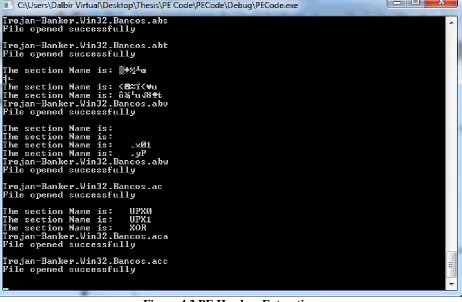
Figure 4.2 PE Headers Extraction

Figure 4.2 shows the output in command prompt window while running the code for feature

extraction. Only the unknown section names are printed on the output window.

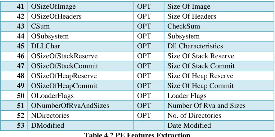
4.4.1 Feature Extraction

This section explains and describes the features extracted from PE files. We have written code to

disassemble the PE file. We have collected 53 features from all the dataset of benign and

malicious files. All 53 features are mentioned and described in Table 4.2.

(Table 4.2 Cont.)

SR No.

Feature Name Header Description

1 FSize File Size

(34)

3 DPf DOS Pages in file

4 DR DOS Relocations

5 DShp DOS Size of header in paragraphs

6 Dmaxp DOS Minimum extra paragraphs

needed

7 Dminp DOS Maximum extra paragraphs

needed

8 Diss DOS Initial (relative) SS value

9 DSPv DOS Initial SP value

10 Dcsum DOS Checksum

11 DIPv DOS Initial IP value

12 Dicsv DOS Initial (relative) CS value

13 Dreltab DOS File address of relocation table

14 DONum DOS Overlay number

15 NSec File No. of Sections

16 DateTime File Date Time

17 FPointerToSymbolTable File Pointer To Symbol Table

18 FNumberOfSymbols File Number Of Symbols

19 FSizeOfOptionalHeader File Size Of Optional Header

20 FCharacteristics File Characteristics

21 USec File No. of Unknown Sections

22 IDll File No. of DLL Function call

23 OMajorLinkerVersion OPT Major Linker Version

24 OMinorLinkerVersion OPT Minor Linker Version

25 SCode OPT Size of Code

26 SIData OPT Size of Initialized Data

27 SUData OPT Size of Uninitialized Data

28 OAddressOfEntryPoint OPT Address Of Entry Point

29 OBaseOfCode OPT Base Of Code

30 OBaseOfData OPT Base Of Data

31 OImageBase OPT Image Base

32 OSectionAlignment OPT Section Alignment

33 OFileAlignment OPT File Alignment

34 OMajorOperatingSystemVersion OPT Major Operating System Version 35 OMinorOperatingSystemVersion OPT Minor Operating System Version

36 MImageVer OPT Major Image Version

37 OMinorImageVersion OPT Minor Image Version

38 OMajorSubsystemVersion OPT Major Subsystem Version 39 OMinorSubsystemVersion OPT Minor Subsystem Version

(35)

41 OSizeOfImage OPT Size Of Image

42 OSizeOfHeaders OPT Size Of Headers

43 CSum OPT CheckSum

44 OSubsystem OPT Subsystem

45 DLLChar OPT Dll Characteristics

46 OSizeOfStackReserve OPT Size Of Stack Reserve

47 OSizeOfStackCommit OPT Size Of Stack Commit

48 OSizeOfHeapReserve OPT Size Of Heap Reserve

49 OSizeOfHeapCommit OPT Size Of Heap Commit

50 OLoaderFlags OPT Loader Flags

51 ONumberOfRvaAndSizes OPT Number Of Rva and Sizes

52 NDirectories OPT No. of Directories

53 DModified Date Modified

Table 4.2 PE Features Extraction

Features like USec, IDll and DModified are the features, which were created using the data

obtained from PE headers. USec feature is for calculating number of unknown section name in

PE file. A counter representing USec feature is initialized and incremented if a section name

obtain from PE file is other than common name like .text, .data, .pdata, .rdata, .rsrc, .reloc, .tls,

.idata, .edata, CODE, DATA or BSS. Similarly, IDLL is for counting number of dlls called in

Import directory. DModified is the modification date of PE file. This feature is collected from

the properties of the PE file.

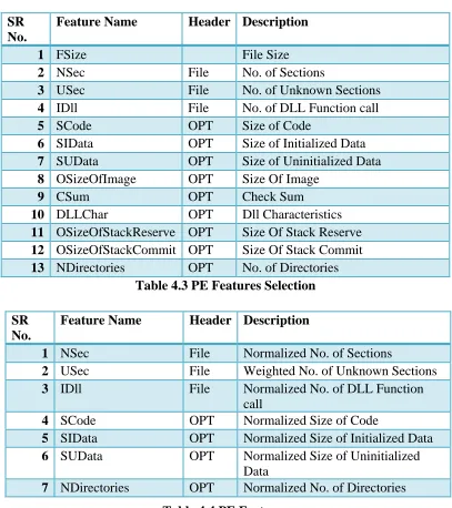
4.5 Feature Selection

All 53 extracted features were considered as initial set of features. Several experiments were

carried out using this set of features but the accuracy obtained after applying data mining

techniques was average. So, to improve the performance and accuracy of clustering with

(36)

giving useful information. Thus we have selected 13 features, which are mentioned and

described in Table 4.3.

SR No.

Feature Name Header Description

1 FSize File Size

2 NSec File No. of Sections

3 USec File No. of Unknown Sections

4 IDll File No. of DLL Function call

5 SCode OPT Size of Code

6 SIData OPT Size of Initialized Data

7 SUData OPT Size of Uninitialized Data

8 OSizeOfImage OPT Size Of Image

9 CSum OPT Check Sum

10 DLLChar OPT Dll Characteristics

11 OSizeOfStackReserve OPT Size Of Stack Reserve 12 OSizeOfStackCommit OPT Size Of Stack Commit 13 NDirectories OPT No. of Directories

Table 4.3 PE Features Selection

Table 4.4 PE Features

Now for better understanding of the data, various features were normalized and given weightage.

Normalization helps in comparing the values for different data sets in a way that it eliminates the

effects of certain gross influences. There were some features in our list of selected features

whose data may vary according to the size of files. Thus for better comparison we have SR

No.

Feature Name Header Description

1 NSec File Normalized No. of Sections

2 USec File Weighted No. of Unknown Sections

3 IDll File Normalized No. of DLL Function

call

4 SCode OPT Normalized Size of Code

5 SIData OPT Normalized Size of Initialized Data 6 SUData OPT Normalized Size of Uninitialized

Data

(37)

normalized the features by dividing the data with its file size. We have also given more

weightage to a feature by multiplying its data with constant integer value hundred. The below

mentioned Table 4.4 contains normalized and weighted features.

4.6 Clustering Algorithm

The clustering algorithm forms group or clusters such that member inside a cluster are similar,

and distinct from the objects in other clusters. For statistical analysis of data, clustering method

is used frequently in the field of data mining. The cluster or groups can be formed, by using

various algorithms that differ in the criteria. The criteria used for forming clusters may include

groups with small distances among the data, dense areas, intervals or particular statistical

distributions [23].

We have used hierarchical, K-mean and self-organizing map clustering algorithm for our data

analysis. The notion of each of the clustering algorithm is different and varies significantly in

their properties.

4.6.1 Hierarchical Learning Algorithm

Hierarchical clustering is an example of connectivity models, which uses distance connectivity to

create groups or clusters. The hierarchy is a tree of clusters, which contains a node as child

(38)

We have used agglomerative hierarchical cluster analysis that is already implemented in Matlab.

The hierarchical algorithm distinguishes every pair of data in dataset. Then it links the pair of

data in close space using the distance criteria that is generated by distinguishing every pair of

data in dataset. In next step a binary tree is formed using data paired into binary clusters. At last,

the clusters were created either by finding natural clusters in the binary tree or by using cutting

off criteria [25].

The function pdist calculates the Euclidean distance between each data pair to distinguish every

pair of data in dataset. The linkage function clusters data into binary tree and dendogram

function helps to view the binary cluster tree graphically for better understanding. The function

cluster is applied to find cut in tree to form clusters either naturally or by giving arbitrary cutoff

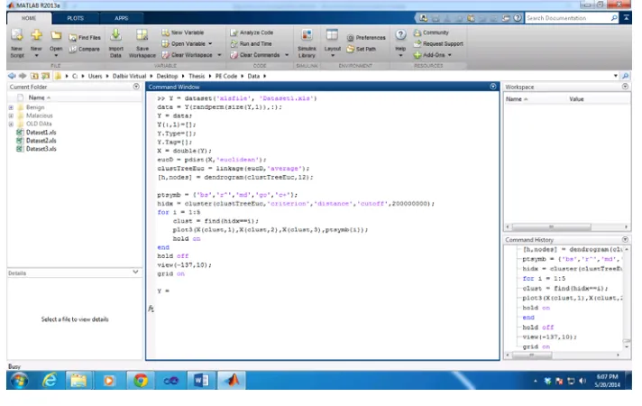
value in function itself. Figure 4.3 shows the code written in Matlab for hierarchical clustering.

Figure 4.3 Hierarchical Matlab Code

As mentioned in the above Hierarchical Matlab code, we used distance cutoff to create clusters

(39)

4.6.2 K-mean Learning Algorithm

K-mean is an example of partition based clustering algorithm. The k-mean algorithm forms

clusters from the data by allocating an index number to each observation according to their mean

value. Each cluster is created or given same index number with nearest mean value. Unlike

hierarchical clustering, k-mean creates cluster on single level and using each observation rather

than similarities or dissimilarities between data pair. Thus k-mean is more suitable and efficient

for cluster analysis of large datasets [26].

K-mean treats each observation in the data as unique. It creates partition in which objects within

each cluster are similar, and distinct from the objects in other clusters [27]. The centroid of the

cluster is calculated by the sum of distances from all data and it helps to increase the efficiency

of the cluster. K-mean iteratively improves by minimizing the sum of distances of each data from

its clusters centroid. The algorithm iterates until the sum of distances of data from centroid

cannot be reduced further. Thus the resultant clusters were compact and well separated as

possible.

The k-mean algorithm is already implemented in Matlab. As explained earlier, k-mean algorithm

returns index of the clusters. Figure 4.4 represents the code written in Matlab to use k-mean

(40)

Figure 4.4 K-mean Matlab Code

As mentioned in Figure 4.4 we asked the K-mean algorithm to create 10 clusters at maximum.

We came up with cluster number 10 by trial and error. When number of clusters was increased,

empty clusters were created and when the number of clusters was decreased, there was

significant drop in the accuracy.

4.6.3 Self Organizing Mapping Algorithm

The SOM is an excellent tool in exploratory phase of data mining [18]. SOM is a type of

artificial neural network (ANN) that produces discrete clusters by training the network using

unsupervised learning. SOM uses neighborhood function to preserve the topological properties

of input [28]. SOM groups the data based on similarity between objects. Thus it can be used to

create clusters of benign and malicious objects.

The other version of SOM training, which we have used is called batch algorithm. It presents

whole dataset to the network then algorithm determines winning neuron and updates each weight

(41)

Matlab has a tool, which can be used to run SOM algorithm. As shown in Figure 4.5 we can first

create grid and train data using batch algorithm in Figure 4.6.

Figure 4.5 Neural Network Architecture

(42)

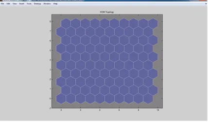
SOM creates different type of plots for the better understanding of analysis results. Figure 4.7

gives view of SOM topology.

Figure 4.7 SOM Topology

Figure 4.8 shows SOM neighbor connections

(43)

Figure 4.9 depicts SOM neighbor weight distances.

Figure 4.9 SOM Neighbor Weight Distances

Figure 4.10 gives overview of SOM weight planes.

(44)

Figure 4.11 shows SOM weight positions.

Figure 4.11 SOM Weight Positions

Figure 4.12 gives gist on SOM sample hits.

(45)

In SOM weight distance and planes, the weights were closer if it is indicated by light colors and

the distances were larger if it is indicated by darker band. The color difference distinguishes

between the data points weight and distance.

Figure 4.13 represents the code written in Matlab to use SOM algorithm.

Figure 4.13 SOM Matlab Code

As mentioned in the code, SOM algorithm is first trained and output is saved in Matlab. Then

(46)

CHAPTER 5: OUTCOME OF PROJECT

5.1 Experimental Tools and Environment

This section gives an overview on the tools and environment used for the thesis project.

5.1.1 Microsoft Visual Studio

Visual Studio (VS) is a comprehensive collection of tools and services that helps to create a wide

variety of applications [30]. VS is an integrated development environment (IDE) from Microsoft

that supports different programming languages that allows to write, edit or debug code. We have

created Visual C++ (VC++) project using Microsoft VS to disintegrate or collect PE headers

values from executables and dynamic link library files. Microsoft VC++ implements both C and

C++ compiler and specific tools for integration with VS IDE. We have added several packages

and in-built libraries to write code.

5.1.2 Matlab

Matlab is a language with strong abstraction and easy to use visual interface that can be used for

data analysis, developing algorithm, creating models and applications, for programming and

more. The built-in tools, mathematical functions and algorithms help to explore multiple

approaches and get the result faster. Matlab can be used in various fields but not limited to

computational biology, computational finance, simulation, image and video processing, signal

(47)

5.1.3 VMware Workstation

VMware workstation is a hypervisor, which helps users to create one or more virtual machines

(VM) on a single system. Each VM can run different operating systems such as Linux, Ubuntu,

and different version of Windows. VMware workstation supports host network, share hard

drives, and USB devices with VM [32].

VM plays an integral part in malware analysis. VM enables us to create a virtual environment

with all the necessary tools and applications required according to our need. We have used

VMware workstation version 10.0.1 build-1379776 with windows 7 operating system and 5.7

GB RAM.

VM has a very useful and important feature called snapshot, which saves the state of machine.

We can create snapshots of our VM that will save all the data, application installed and settings

of the operating system at that very moment. Once the snapshot is created we can restore the

saved state whenever it is necessary. For example, if a malware affects the system we can restore

the machine to its stored state by restoring a snapshot. The snapshot feature saves lot of time and

work while doing malware analysis.

5.2 Experimental Results

Experiment 1:

(48)

Algorithm: Hierarchical algorithm

Output: Figure 5.1 represent the binary tree of hierarchical algorithm on dataset1 in

dendogram form with top twelve nodes. We have created dendogram with cutoff as the

dataset is very large and dendogram representing the complete dataset was visually not clear.

Now, to go one step further we have created clusters and represented in Figure 5.2. Similarly,

for clearer view we have represented few cluster and data points in the graph.

(49)

Figure 5.2 Experiment 1 Plot

Clusters were created using cutoff on distance criteria. Table 5.1 represents the 28 clusters

created with useful details. Column “Value” represents the number of executables with type

benign or malicious and “Percentage” gives the idea on percent of executables type in cluster.

(Table 5.1 Cont.)

Hierarchical on Datset 1

Cluster Executable Value Percentage Cluster Executable Value Percentage Cluster Executable Value Percentage

1 Benign 0 0.00% 11 Benign 8 50.00% 20 Benign 11127 51.01%

Malacious 1 100.00% Malacious 8 50.00% Malacious 10686 48.99%

(50)

10 Benign 32 94.12%

Malacious 2 5.88%

Table 5.1 Experiment 1 Clusters

Figure 5.3 Experiment 1 Graph

Analysis: There were around 22,172 executables in dataset. After applying hierarchical

algorithm, 28 clusters were created using distance cutoff. Hereafter analyzing the cluster data

we found that around 10,702 executables were clustered wrongly, which results in accuracy

(51)

Now we further analyze the results or clusters obtained after applying Hierarchical algorithm

on Dataset1. We have created a graph in Figure 5.3 for better understanding of our results.

The X-axis represents the cluster with 50% to 100% accuracy rate divided in four groups.

The Y- axis represents the percentage of the clusters that belongs to the groups mentioned in

X-axis. Each of the bar has a percentage label which represents the percentage of executables

from Datset1 that belongs to the group. Moreover, from the figure 5.3 we observe that

98.54% of executables from Dataset1 have 50-79.99% accuracy and less than 20% of

clusters belong to this group. Thus, we know that most of the executables from Dataset1

belong to less than 20% of clusters and has efficiency between 50% to 79.99% and rest of the

clusters have only 1.46% of executables. Hence, the efficiency obtained in this experiment is

very low.

Experiment 2:

Input: Dataset1

Algorithm: K-means algorithm

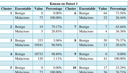
Output: Figure 5.3 represent centroid of the clusters created using kmean algorithm. Table

(52)

Figure 5.4 Experiment 2 Plot

Kmean on Datset 1

Cluster Executable Value Percentage Cluster Executable Value Percentage

1 Benign 0 0.00% 6 Benign 64 73.56%

Malacious 73 100.00% Malacious 23 26.44%

2 Benign 19 79.17% 7 Benign 7 63.64%

3 Benign 333 3.06% 8 Benign 50 79.37%

4 Benign 10733 98.89% 9 Benign 0 0.00%

5 Benign 0 0.00% 10 Benign 17 23.29%

(53)

Figure 5.5 Experiment 2 Graph

Analysis: There were around 22,172 executables in dataset that is used for clustering. After

applying K-mean algorithm 10 clusters are created. The number of clusters were decided by

trial and error and given to the algorithm. If we create more than 10 clusters than empty

clusters were created and if we give less than accuracy is reduced significantly. After

analyzing the details of each cluster given in Table 5.2, we found that out of 22,172 around

515 executables were wrongly clustered, which gives accuracy of 97.68%. This accuracy is

significantly more than obtained in experiment1.

Similar to Experiment 1 we have created a graph in Figure 5.5 for better understanding and

analysis of the results or clustered obtained by applying K-mean algorithm on Dataset1. As

(54)

of 90-99.99% but out of the clusters created approximately 20% of clusters have this kind of

efficiency.

Experiment 3:

Input: Dataset1

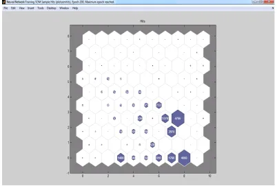
Algorithm: SOM algorithm

Output: A gridof 10 X 10 is created according to the input. Figure 5.4 represents the sample

hits, which means it shows the number of elements in each cluster. Table 5.3 gives the details

of each cluster.

(55)

(Table 5.3 Cont.)

SOM on Datset 1

Cluster Executable Value Percentage Cluster Executable Value Percentage Cluster Executable Value Percentage

(56)

29 Benign 0 0.00%

Malacious 3 100.00%

Feature selection and clustering for malicious and benign software characterization

ScholarWorks@UNO

ScholarWorks@UNO

Feature selection and clustering for malicious and benign

Feature selection and clustering for malicious and benign

software characterization

software characterization

ACKNOWLEDGEMENT

TABLE OF CONTENTS

LIST OF TABLES

LIST OF FIGURES

ABBREVIATIONS

ABSTRACT

CHAPTER 1: PROJECT OVERVIEW

1.1

Introduction

1.2

Statement of problem

1.3

Project Objective

1.4

Project Scope

1.5

Limitation

1.6

Thesis Structure

Background:

Related Work:

Proposed Methodology:

Experiment and outcome of project:

Conclusion and Future study:

CHAPTER 2: BACKGROUND

2.1

Malware and its types

2.2

Introduction to Malware Analysis

2.3

Malware Analysis Techniques

2.4

Introduction to Portable Executable Format

Size Field

Description

Section

Name

Section Description

CHAPTER 3: RELATED WORK

3.1

Malware Detection

3.2

Data Mining

3.3

Discussion and Summary

CHAPTER 4: PROPOSED METHODOLOGY

4.1

Proposed Approach

4.2

Introduction to Data Mining











4.3

Data Collection

4.4

Data Pre-processing

4.4.1

Feature Extraction

4.5

Feature Selection

4.6

Clustering Algorithm

4.6.1

Hierarchical Learning Algorithm

4.6.2

K-mean Learning Algorithm

4.6.3

Self Organizing Mapping Algorithm

CHAPTER 5: OUTCOME OF PROJECT

5.1