UNEMPLOYMENT DYNAMICS IN THE OECD
Michael W. L. Elsby, Bart Hobijn, and Ay¸
segül ¸
Sahin
January 2012
Abstract
We provide a set of comparable estimates for the rates of in‡ow to and out‡ow
from unemployment using publicly available data for fourteen OECD economies.
Using a novel decomposition that allows for deviations of unemployment from its
‡ow steady state, we …nd that ‡uctuations in both in‡ow and out‡ow rates
con-tribute substantially to unemployment variation within countries. Anglo-Saxon
economies exhibit approximately a 15:85 in‡ow/out‡ow split to unemployment
variation, while Continental European and Nordic countries display closer to a
45:55 split. In all economies increases in in‡ows lead increases in unemployment,
* Elsby: University of Edinburgh; Hobijn: Federal Reserve Bank of San Francisco, VU
University Amsterdam, and Tinbergen Institute; ¸Sahin: Federal Reserve Bank of New York.
We would like to thank anonymous referees, Regis Barnichon, Wilbert van der Klaauw,
Emi Nakamura, Simon Potter, Gary Solon, participants at the New York/Philadelphia
Work-shop on Quantitative Macroeconomics 2008, Midwest Macroeconomics Conference 2009,
Re-cent Developments in Macroeconomics Conference 2009, EEA Conference 2009, CREI/Kiel
Conference on Macroeconomic Fluctuations and the Labor Market 2009 for helpful
com-ments, and Joseph Song for outstanding research assistance. The views expressed in this
paper are those of the authors and do not necessarily re‡ect those of the Federal Reserve
Bank of New York, the Federal Reserve Bank of San Francisco or the Federal Reserve System.
An Excel spreadsheet with all the data, calculations, and results presented in this paper is
available for download at www.frbsf.org/economics/economists/bhobijn/. Thanks to Jonas
Staghøj for pointing out a coding error in a previous version of the spreadsheet.
E-mail addresses for correspondence: [email protected]; [email protected];
1
Introduction
Unemployment rates among developed economies have varied substantially both across time
and across countries over the last 40 years. This variation in unemployment may occur as a
result of variation in the rate at which workers ‡ow into the unemployment pool, variation
in the rate at which unemployed workers exit the unemployment pool, or a combination
of the two. The relative contributions of changes in in‡ow and out‡ow rates to changes
in unemployment have been abundantly documented for the U.S.1 Less is known, however,
about the driving forces of unemployment variation in other countries. Such a question is
of interest because of the considerable variation in unemployment that has been observed
in developed economies in recent decades, notably in Continental Europe. In this paper, we
provide a detailed analysis of unemployment ‡ows for fourteen developed economies using
publicly available data.
In the …rst part of our analysis we describe how it is possible to derive measures of the
rates of in‡ow2 to and out‡ow from the unemployment pool using annual data from the
OECD. To do this, we generalize the method developed by Shimer (2007), which makes use
of time series for the number employed, the number unemployed, and the number
unem-ployed less than …ve weeks to infer ‡ow hazard rates for the U.S. A limitation that arises
when applying this methodology outside the U.S. is that series on short duration
unemploy-ment can be noisy for countries in which short durations account for a small proportion
of overall unemployment, such as in Continental Europe. To address this, we develop a
method that exploits additional data on unemployment at higher durations to construct a
set of comparable time series for the unemployment in‡ow and out‡ow rates across countries.
Our measures allow us to document a set of stylized facts on unemployment ‡ows among
developed economies. First, the average level of unemployment in‡ow and out‡ow rates
varies substantially across countries. Interestingly, the results suggest a natural
Nordic economies display high exit rates from unemployment, with monthly hazards that
exceed 20 percent. In stark contrast, out‡ow rates among Continental European economies
are much lower— typically less than 10 percent at a monthly frequency. Symmetrically,
un-employment in‡ow rates also vary considerably across countries. Anglo-Saxon and Nordic
countries exhibit in‡ow hazards that exceed 1.5 percent at a monthly frequency. However, as
with the observed levels of out‡ow rates, monthly in‡ow rates among Continental European
economies are again much lower at around 0.5 to 1 percent. These observations con…rm the
diagnosis that European labor markets arescleroticin the sense that they display much lower
rates of reallocation of labor, as documented in Blanchard and Summers (1986), Bertola and
Rogerson (1997), Blanchard and Wolfers (2000), and Blanchard and Portugal (2001).
In the second part of our analysis, we pose the question of how much of the observed
vari-ation in unemployment within each country can be accounted for by varivari-ation in the in‡ow
rate into unemployment and variation in the out‡ow rate from unemployment respectively.
To answer this, we provide a method for decomposing changes in the unemployment rate
into contributions due to changes in the ‡ow hazards that can be applied in countries with
very di¤erent unemployment dynamics. Recent literature (Elsby, Michaels, and Solon, 2009;
Fujita and Ramey, 2009; Petrongolo and Pissarides, 2008) has evaluated these contributions
under the assumption that the unemployment rate is closely approximated by its ‡ow steady
state value. Under this assumption, contemporaneous unemployment variation may be
de-composed into contributions related to contemporaneous logarithmic variation in in‡ow and
out‡ow hazards. While this steady state assumption holds as a reasonable approximation
in the U.S., we show that it can be very inaccurate in other developed economies, notably
those of Continental Europe.
Reacting to this we show that, in cases where unemployment deviates from steady state,
current variation in unemployment can be decomposed recursively into contributions due
when unemployment is out of steady state, it can vary as a result of contemporaneous
changes in the in‡ow and out‡ow rates, or as a result of dynamics driven by past changes in
these ‡ow hazards. Using our alternative decomposition, we obtain a much more accurate
characterization of changes in unemployment rates across countries.
Application of our decomposition to our estimated time series for the ‡ow hazard rates
provides us with a second stylized fact on unemployment ‡ows. Among all countries that we
consider, ‡uctuations in both in‡ow and out‡ow rates contribute substantially to
unemploy-ment variations within countries. The relative contribution of each di¤ers across countries,
however. Among Anglo-Saxon economies we …nd approximately a 15:85 in‡ow/out‡ow split
of unemployment variation, a result that echoes recent …ndings for the U.S. over the same
sample period. For Continental European and Nordic countries, however, we observe much
closer to a 45:55 in‡ow/out‡ow split. Thus, a complete understanding of unemployment
variation among our large sample of developed economies requires an understanding of the
determinants of both the in‡ow rate as well as the out‡ow rate.
The …nal part of our empirical analysis uses the estimated ‡ow hazard rates to compute
measures of thenumber of workers ‡owing in and out of the unemployment pool (as opposed
to the hazard rates for these ‡ows).3 A third stylized fact that emerges from these results is
that a geographical partitioning also applies to average worker ‡ows across countries.
Anglo-Saxon and Nordic countries exhibit annual worker ‡ows in and out of unemployment that
comprise more than 15 percent of the labor force. Among Continental European economies,
on the other hand, worker ‡ows typically involve less than 10 percent of the labor force,
echoing the …ndings of Blanchard and Portugal (2001) and Bertola and Rogerson (1997).
We then analyze the dynamic relationship between these worker ‡ows and unemployment
within each country. Using a simple correlation analysis, we document a fourth stylized fact
on unemployment ‡ows among developed economies: The timing of the contributions of
countries. In all economies we observe that increases in in‡ows lead increases in
unem-ployment, whereas out‡ows lag a ramp up in unemunem-ployment, an observation that has been
highlighted for the U.S. in earlier studies.4
Our …ndings that variation in unemployment in‡ows accounts for a substantial fraction of
unemployment variation and is an important leading indicator for changes in unemployment
dovetails with a recent literature on U.S. unemployment ‡ows. A growing trend in modern
macroeconomic models of the aggregate labor market has been to assume that the in‡ow rate
into unemployment is acyclical (Hall, 2005a,b; Shimer, 2005; among others). Reacting to
this, a number of recent studies has cautioned against this trend by documenting evidence for
systematic countercyclical movements in unemployment in‡ows in U.S. data.5 Our …ndings
show that this caution resonates all the more if we wish to understand the considerable
variation in unemployment rates observed outside the U.S.
The remainder of the paper is organized as follows. In section 2 we summarize the OECD
data that we use throughout our analysis. In section 3, we describe our methodology for
inferring the rates of in‡ow to and out‡ow from the unemployment pool using the OECD
data. Application of this methodology provides individual time series for the unemployment
‡ow hazards for each of the fourteen countries in our sample. In section 4, we pose the
question of how much of the variation in unemployment within countries can be accounted
for by changes in the in‡ow and out‡ow rates respectively. To answer this question, we
derive a decomposition of unemployment variation that allows for unemployment to deviate
from steady state. We show that allowing for such deviations is critical for understanding
unemployment ‡uctuations outside the U.S. Section 5 presents evidence on the number of
workers ‡owing in and out of unemployment, and documents stylized facts on the timing
of the impact of worker ‡ows on unemployment changes. Section 6 summarizes and o¤ers
2
Data
Since a large part of our analysis is informed by the available data, we start by discussing
the OECD samples that we use. These are taken from two di¤erent sources. First, we
use annual measures of the unemployment stock by duration, taken from OECD (2010a).6
We then supplement these data with quarterly measures of the aggregate unemployment
rate, taken from OECD (2010b). Both slices of data are based on the labor force surveys
conducted in each of the countries in our sample.
The fourteen economies that we focus on are: Australia, Canada, France, Germany,
Ireland, Italy, Japan, New Zealand, Norway, Portugal, Spain, Sweden, United Kingdom,
and the United States. For all countries relatively long historical quarterly time series are
available for the unemployment rate. Our focus on these economies is primarily driven by
the length of the available requisite series for unemployment by duration. Throughout, we
denote the fraction of the labor force in an unemployment spell of less than d months in
month t by u<d
t .7 For our analysis we use annual time series for u<1t , ut<3, u<6t , and u<12t .
Note that we de…ne these categories inclusively, in the sense that u<3t includes u<1t , and so on. The starting year for the available series varies between 1968 (for the U.S.) and 1986
(for New Zealand and Portugal).8 For all countries, the data end in 2009.
An important advantage of using data from the OECD is that, even though the labor force
surveys of these countries have di¤erent structures, the OECD data have been standardized
to adhere to the same structure. This aids cross-country comparisons of our results.9
3
The Ins and Outs of Unemployment in the OECD
At the heart of our analysis is a set of estimated annual time series of ‡ow hazard rates into
and out of unemployment for fourteen OECD countries. These time series are estimated using
method cannot be applied directly to other OECD countries because the required data are
not available. The extension that we introduce allows us to overcome this limitation and to
produce annual time series for the rates of in‡ow to and out‡ow from the unemployment
pool for a large subset of OECD countries.
3.1
Analytical Framework
The evolution over time of the unemployment rate, which we denote by ut, can be written
as:10
dut
dt =st(1 ut) ftut; (1)
where st is the monthly rate of in‡ow into unemployment, ft is the monthly out‡ow rate
from unemployment, andt indexes months.11 As mentioned above, the data that we use in
the remainder of the paper allow us to infer unemployment ‡ows at an annual frequency.
Thus, we would like to relate the continuous time evolution of unemployment in equation (1)
to the unemployment rates that we observe at discrete annual intervals. Assuming that the
‡ow hazards are constant within years,12 and solving equation (1) forward one year allows
us to do this:
ut= tut + (1 t)ut 12, (2)
where
ut = st st+ft
(3)
denotes the ‡ow steady-state unemployment rate, and
t= 1 e 12(st+ft) (4)
is the annual rate of convergence to steady state. In this way we can relate variation in
underlying ‡ow hazards,st andft. To implement this, however, we need to obtain estimates
of these ‡ow hazards, to which we now turn.
Our method for estimating the out‡ow rateftis an extension of the method popularized
by Shimer (2007). In his study of U.S. unemployment ‡ows, he infers the monthly out‡ow
probabilityFtusing the identity that the monthly change in the unemployment stock is given
by
ut+1 ut=u<1t+1 Ftut. (5)
Hereu<1
t+1 denotes the stock of unemployed workers with duration less than one month, and
hence re‡ects the ‡ows into unemployment; Ftut re‡ects the ‡ows out of unemployment.
Solving for the monthly out‡ow probability, one obtains13
Ft= 1
ut+1 u<1t+1 ut
. (6)
The monthly out‡ow probability is then related to the associated monthly out‡ow hazard
rate, ft<1, through
ft<1 = ln(1 Ft). (7)
3.2
Estimation of Flow Hazard Rates
Duration Dependence and Estimation of the Out‡ow Rate In what follows we will
see that the estimate of the out‡ow rate implied by equation (6) works well for countries
in which the out‡ow rate from unemployment is relatively high, such as the U.S. However,
in countries that exhibit low exit rates, such as those of Continental Europe, estimates
based on equation (6) can be substantially noisy. The simple reason is that low out‡ow
rates imply that very few unemployed workers at a point in time are in their …rst month of
unemployment, which increases the sampling variance of the estimate of u<1t+1, and in turn
Our approach to this problem is to use the additional unemployment duration data
available from the OECD to increase the precision of our estimate of ft in countries where
the out‡ow rate is low. To see how this may be done recall that the OECD data also report
the unemployment stock at durations higher than one month. It follows that, analogous to
the method detailed above, it is possible to write the probability that an unemployed worker
exits unemployment within d months as
Ft<d = 1 ut+d u <d t+d ut
. (8)
As before, this can be mapped into an out‡ow rate estimate given by
ft<d = ln(1 Ft<d)=d: (9)
Given the available data, we can estimateft<d for d= 1;3;6;12.15
It is important to clarify the interpretation of the out‡ow rate measures ft<d. It is
tempting to interpretf<d
t as the out‡ow rate for unemployed workers of durationd. However,
that is not an accurate interpretation. Rather, it is the hazard rate associated with the
probability that an unemployed worker at timet completes her spell within the subsequent
d months.
These four measures, ft<1; ft<3; ft<6; and ft<12, are not necessarily estimates of the same out‡ow rate. Only in the case where the out‡ow hazard is unrelated to the duration of an
unemployment spell, i.e. if there is no duration dependence in out‡ow rates, are all four
measures consistent estimates of the aggregate out‡ow rate from unemployment, de…ned
as the average out‡ow rate among the entire unemployed population. However, if there is
duration dependence in unemployment out‡ow rates in a given country, then estimates based
For example, imagine that there exists negative duration dependence whereby the out‡ow
rate declines with duration.16 In such an environment, we would expect to observe f<1
t > ft<3 > ft<6 > ft<12. To see why, consider the version of equation (8) which expresses the
fraction of the unemployment stock in month t that exits within the next three months.
The remaining unemployed workers that do not exit over these subsequent three months
increasingly will be comprised of unemployed workers with low out‡ow rates, i.e. the high
duration unemployed. This process of dynamic selection will imply that excessive weight
will be placed on the low out‡ow rates of high duration unemployed workers in the estimate
of ft<3, generating a downward bias in its estimate of ft. This argument applies even more
strongly to the estimates of ft<6 and ft<12.17
In light of this, we formally test for the presence of duration dependence in out‡ow rates
by testing the hypothesis that ft<1 =ft<3 = ft<6 = ft<12. The formal details are described in the Appendix, but our general approach is as follows. First, we derive the asymptotic
distribution of the unemployment rates by duration as well as for the unemployment rates
themselves. We then apply the Delta method to compute the joint asymptotic distribution
of the out‡ow rate estimates ft<d with d = 1;3;6;12. This allows us to formulate a simple
Chi-squared test of the null hypothesis of no duration dependence.
It should be noted that we test for a very broad de…nition of duration dependence.
As has been emphasized since Kaitz (1970), duration dependence can arise through two
channels. “True”duration dependence refers to the case where unemployment duration has
a causal e¤ect on the out‡ow rates of individual workers. In contrast, “spurious” duration
dependence refers to the process of dynamic selection whereby workers with high exit rates
leave unemployment faster than those with low exit rates, thereby generating a negative
correlation between duration and out‡ow rates (Salant, 1977). Our hypothesis test is not
intended to distinguish between these two sources of duration dependence, but rather to
di¤erent from one another. Thus, the duration dependence we test for can arise due to either
dynamic selection or true duration dependence or both.
For those countries for which we reject the hypothesis of no duration dependence, we
follow the recent U.S. literature in using ft<1 as our estimate of the unemployment out‡ow
rate, as this measure provides the least biased estimate of the average out‡ow rate in the
presence of duration dependence. For countries with weak evidence for duration dependence
for which we do not reject the null, we make use of all the additional information on the
out‡ow rate contained inf<3
t ; ft<6;and ft<12 in order to obtain a more precise estimate offt.
Speci…cally, we use our estimates of the asymptotic distribution of the out‡ow rate estimates,
ft<1; ft<3; ft<6; and ft<12 to compute an optimally weighted estimate of the out‡ow rate that
minimizes the mean squared error of the estimate.18
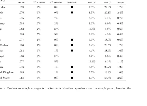
The results of the hypothesis test are reported in Table 2. While we …nd signi…cant
evidence of duration dependence in Anglo-Saxon and Nordic countries and Japan, we do not
observe signi…cant evidence among the Continental European countries in our sample.19 It is
natural to ask whether this conclusion is supported by the results of microeconometric studies
that estimate duration dependence for speci…c European economies. A particularly useful
summary of this literature is reported by Machin and Manning (1999, Table 6). They show
that the evidence for duration dependence among European economies is quite inconclusive.
Estimates of duration dependence in Germany and Spain, for example, di¤er across studies,
with evidence found for negative, positive and negligible duration dependence reported. Our
conclusion of limited evidence for duration dependence lies at the midpoint of this array.
A clearer consensus emerges for France and the U.K. For France, the literature …nds very
little evidence for duration dependence, at least within the …rst year of the unemployment
spell. In contrast, for the U.K., the literature in general …nds evidence for negative duration
dependence. Our estimates are in line with these conclusions.
across countries. In their own analysis, Machin and Manning (1999) …t a Weibull
dura-tion model to the duradura-tion structure of unemployment across countries. They report weak
negative duration dependence in France and Spain in the 1990s, but strong negative
du-ration dependence in Australia, the U.K. and the U.S. in the 1980s and 1990s. Using a
similar approach on OECD data, Hobijn and ¸Sahin (2009) also …nd little evidence of
dura-tion dependence among Continental European economies, but substantial evidence among
economies with high unemployment out‡ow rates.
The result of our hypothesis test is that we usef<1
t as our estimate of the out‡ow rate for
the Anglo-Saxon countries in our sample and the optimally weighted average offt<1; ft<3; ft<6;
and ft<12 for the remaining countries.
Temporal Aggregation Bias and Estimation of the In‡ow Rate Given our estimate
of the out‡ow rate, we compute the in‡ow rate st using the method pioneered by Shimer
(2007). In particular, note that the expression for the annual unemployment rate in equation
(2) is simply a nonlinear equation in the unemployment rates, ut+12 and ut, and the ‡ow
hazard rates,st and ft. We can thus solve equation (2) for the in‡ow rate.
As emphasized by Shimer (2007) and subsequent work based on his method, this estimate
of the in‡ow rate is robust to temporal aggregation bias in the measurement of unemployment
in‡ows. In particular, since equation (2) is inferred from solving forward the continuous-time
di¤erential equation for the evolution of the unemployment rate, it accounts for the fact that
workers who ‡ow into unemployment after one period’s survey may exit prior to the next
period’s survey, ‡ows that would be missed in discrete-time data. Correcting for temporal
aggregation bias in the in‡ow rate is particularly important the context of the OECD data,
since the data are available at an annual frequency, in contrast to the monthly data that are
available for the U.S.20
Interestingly, estimation of the out‡ow rate from unemployment is not subject to a
in equation (6). This is just the complement of the probability that those unemployed at
timetremain unemployed by timet+ 1. If there were a time aggregation problem, a concern
would be that the data fail to pick up on workers who exit unemployment after one period’s
survey, but who re-enter prior to the next period’s survey. However, the measure of the
out‡ow probability in equation (6) does not miss such transitions: Any worker who followed
this path would be identi…ed as short-term unemployed in the second survey, and therefore
correctly counted as an out‡ow.
Nevertheless, it still could be the case that the measure of the out‡ow probability in
equation (6) misses multiple exits from unemployment within the period (e.g. out after …rst
survey, in again, out again, in again prior to next survey). We will see that the in‡ow rate
in practice is very small in comparison to the out‡ow rate for most countries in our sample,
so that the probability of such multiple transitions for these countries is likely to be small.21
It is important to note, however, that our approach estimates average ‡ow rates taken over
potentially very heterogeneous populations. This point is especially apparent in economies
that have made widespread use of temporary, or …xed-term, contracts, such as Spain.22
The existence of these contracts can give rise to a fraction of workers who experience very
high rates of turnover, and for whom time aggregation is a more acute problem. These
important sources of heterogeneity cannot be gleaned from data on the duration structure
of unemployment that we use throughout the paper. Uncovering the di¤erential role of time
aggregation across di¤erent subgroups of the labor market is therefore an important avenue
for future research.
3.3
Evidence from OECD Data
The average unemployment in‡ow and out‡ow hazards over the sample periods for the whole
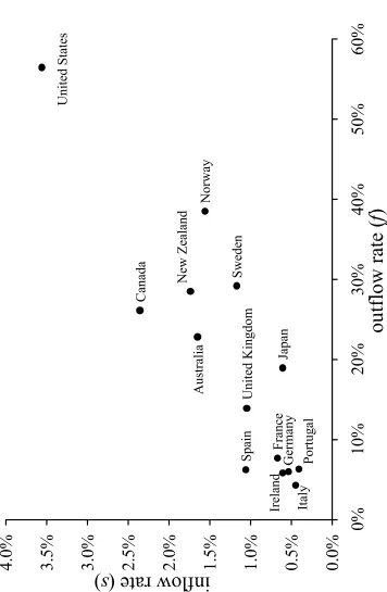
sample of countries are reported in Table 2. A striking observation from these results is the
this point is in Figure 1, which displays the average values ofstand ft from Table 2 in graph
form. Interestingly, one can discern a natural partition of developed economies between
Anglo-Saxon, Nordic and Continental European economies.
Figure 1 reveals very high out‡ow rates among the Anglo-Saxon and Nordic economies.
Among these countries the average monthly unemployment out‡ow hazard exceeds 20
per-cent. The economies of Continental Europe stand in stark contrast. Unemployment out‡ow
rates in these economies lie below 10 percent at a monthly frequency. A similar picture
develops for the estimates of the in‡ow rates in Figure 1. We observe high unemployment
in‡ow hazards among the Anglo-Saxon and Nordic economies, which typically lie above 1.5
percent on a monthly basis. Likewise, in‡ow rates among the European economies are again
much lower at around 0.5 to 1 percent per month.23
Figure 1 also shows that there are both extremes and intermediate cases that are
un-derstated in this Anglo-Saxon/Nordic/Continental Europe taxonomy. For Japan, while the
average unemployment out‡ow rate of 19 percent is similar to those in Anglo-Saxon and
Nordic economies, its in‡ow rate is more comparable to those of Continental Europe.
An-other intermediate case is the U.K., which displays unemployment ‡ows that lie halfway
between the Anglo-Saxon and the Continental European models. Perhaps the most striking
observation, however, is the outlier status of the U.S. With an average monthly
unemploy-ment out‡ow rate of nearly 60 percent and an average in‡ow rate of 3.5 percent, it exhibits
transition rates at least 50 percent larger than the remainder of our sample of countries.
Figures 2 and 3 display the time series for the in‡ow and out‡ow hazards for each country
in our sample. The transition rates are plotted on log scales since, as emphasized in the
literature on unemployment ‡ows, and as we will con…rm in what follows, it is the logarithmic
variation in st and ft that places them on an equal footing with respect to ‡uctuations in
the unemployment rate.
unem-ployment ‡ows, there is also substantial variation in unemunem-ployment ‡ow hazards over time
within countries. Although there is a great deal of information contained in these …gures,
a number of observations come to light. First, there are important di¤erences in the
fre-quency of ‡uctuations in unemployment ‡ows across economies. Among the Anglo-Saxon
economies, a clear cyclical pattern is present, suggesting a substantial high frequency
com-ponent to unemployment ‡uctuations in these countries. Among other economies, however,
the variation in st and ft occurs at a much lower frequency, and it is hard to di¤erentiate
cycle from trend.
Figures 2 and 3 are also indicative of how the relative contributions of variation in the
in‡ow and out‡ow rates di¤er across countries. Speci…cally, the Anglo-Saxon economies
appear to display relatively more variation in the out‡ow rate from unemployment, a point
that has been emphasized in recent literature for the U.S. However, inspection of the time
series for the Nordic and European economies reveals greater variation in the in‡ow rate,
suggesting about an equal contribution of the ins and the outs to unemployment variation
in these countries.
Figures 2 and 3 also provide a sense of the degree to which these stylized facts have held
true in the most recent recession. In many respects, historical di¤erences in unemployment
dynamics between Anglo-Saxon and Continental European economies have been echoed in
recent data. Inspection of the time series for the ‡ow hazards after 2007 reveals that, as in the
past, the recent rise in unemployment has been associated more with rises in unemployment
in‡ows in Continental European economies, and with declines in rates of out‡ow in
Anglo-Saxon countries. Figures 2 and 3 do point to one stark feature of the recession, however:
The out‡ow rate from unemployment in the U.S. fell precipitously to reach a historic low, a
point noted by many observers of the Great Recession in the U.S. (for example, see Elsby,
Hobijn and ¸Sahin, 2010). An advantage of the cross-country estimates in Figures 2 and 3
rates of exit from unemployment in the U.S., the level of the out‡ow rate witnessed recently
in the U.S. still dwarfs those observed in Continental Europe.
Of course, this visual impression is only suggestive of the relative contributions of the
in‡ow and out‡ow hazards to unemployment variation; we address this issue more formally
in section 4. Before we do so, we …rst compare our estimates of unemployment transition
rates with those reported in related literature.
3.4
Relation to Existing Evidence
Unemployment ‡ows for the U.S. have been extensively studied in the literature. Almost all
of these studies, including Elsby, Michaels, and Solon (2009), Fujita and Ramey (2009) and
Shimer (2007), are based on data from the Current Population Survey. Since the OECD
data that we use are also based on the same survey data, the levels of our estimated ‡ow
hazards are in line with these previous estimates.24
The cross-country analysis of ‡ow rates that is most closely related to the results in
this paper is Hobijn and ¸Sahin (2009). They use GMM to estimate average job-…nding and
separation rates for a broader sample of countries. Since they focus on average ‡ow hazards,
their analysis does not address the dynamic properties of the evolution of unemployment in
these countries. The average ‡ow transition rates that they obtain using their estimation
method are almost identical to those documented in Table 2.
The time series plotted in Figures 2 and 3 for countries other than the U.S. also are
qualitatively similar to previous results based on microdata for individual countries. Our
estimates for the U.K. are consistent with the declining employment to unemployment (E–
U) and rising unemployment to employment (U–E) transition rates estimated using U.K.
Labour Force Survey data from the early 1990s on (Bell and Smith, 2002; Gomes, 2008;
and Petrongolo and Pissarides, 2008). The trends we …nd for Germany are consistent with
transition rate and a decline in the U–E hazard in the early 1990s. In addition, the estimated
time series for Spain correspond very closely to those reported in Petrongolo and Pissarides
(2008) using Spanish Labor Force Survey data. Reichling (2005) reports estimates of the
separation rate for a set of countries (see his Table 5) and also emphasizes that the separation
rate is lower in European countries than in the U.S.
There are also several cross-country studies that provide structural estimates of search
models that include estimated ‡ow hazards. Two examples of these are Ridder and van
den Berg (2003) and Jolivet, Postel-Vinay and Robin (2006). Because they are based on
structural models, the estimated transition rates in these papers do not correspond exactly to
the ‡ow rate concept we use here. However, the qualitative ranking of countries in terms of
the levels of in‡ow and out‡ow rates are very similar to ours. For example, Italy is estimated
to have the smallest out‡ow rate, the U.S. the highest, with the U.K lying between the U.S.
and the Continental European countries.
4
Decomposing Unemployment Fluctuations
In this section, we formulate and apply a formal decomposition of changes in unemployment
into parts due to changes in the in‡ow and out‡ow rates for each country. Our decomposition
allows for deviations of the actual unemployment rate from its ‡ow steady-state value. We
show that allowing for such deviations is important for understanding unemployment
‡uc-tuations in many, especially European, countries. We use the annual time series on in‡ow
and out‡ow rates, presented above, to conduct this decomposition. Because we use annual
data in what follows, time, t, is denoted in years rather than months in the remainder of
4.1
Analytical Framework
As mentioned above, an important aim of this paper is to understand the proximate driving
forces behind variation in unemployment rates across countries. As previous literature has
shown, such a task is relatively straightforward for the U.S.25 The reason is that
unem-ployment dynamics are uncommonly rapid in the U.S.— that is, st+ft is a relatively large
number in the U.S. The formal implication of this is that the rate of convergence of the
unemployment rate to its ‡ow steady state value in equation (2), t = 1 e 12(st+ft), is
very close to one in the U.S. In this case, the unemployment rate can be approximated very
closely by its ‡ow steady state value,
ut ut = st st+ft
, and t 1: (10)
As emphasized in Elsby, Michaels and Solon (2009), log di¤erentiation of the latter implies
dlnut (1 ut)[dlnst dlnft]: (11)
Thus, in countries with labor markets characterized by fast unemployment dynamics, a
simple decomposition of unemployment variation presents itself: The relative contributions
of the in‡ow and out‡ow rates to unemployment variation can be gleaned from comparing
the contemporaneous logarithmic variation in the two ‡ow hazard rates.
Based on the evidence we found above, one might anticipate that the approximations
that underlie the decomposition of unemployment variation based on (11) work well among
the Anglo-Saxon and Nordic economies, which display relatively high rates of in‡ow and
out‡ow. However, the evidence also suggests that there is good reason to hesitate in applying
equation (11) as a decomposition of unemployment variation in Continental Europe. The
reason is that the unemployment ‡ow hazards in these economies are very low, especially
steady-state unemployment rate is therefore likely to be a poor approximation to the actual
unemployment rate.
Reacting to this, we devise a decomposition of unemployment changes that holds even
when unemployment is out of steady state. Our approach uses equation (2) as its starting
point. We show in the Appendix that a log-linear approximation to (2) allows us to express
the log change in the unemployment rate recursively as
lnut t 1 1 ut 1 [ lnst lnft] +
1 t 2
t 2
lnut 1 . (12)
This decomposition distinguishes between changes in the steady state due to current changes
in the in‡ow and out‡ow rates, and changes in the unemployment rate due to deviations
from the steady state caused by past changes in the ‡ow rates.
A number of aspects are worth noting about equation (12). First, if unemployment
dynamics are very fast, so that st+ft is high and t is close to one for all t, then equation
equation (12) reduces to the steady-state decomposition implied by (11). In addition, a
particularly intuitive way of understanding (12) is to consider the case where t = for
all t. In that case, the log change in the unemployment rate in (12) is a distributed lag of
contemporaneous and past log changes in the in‡ow rate st and the ft. This highlights a
potential pitfall of applying the steady-state decomposition in (11) to unemployment ‡ows
in economies, such as those of Continental Europe, with slow unemployment dynamics:
Out of steady state, contemporaneous variation in the unemployment rate is driven both
by contemporaneous as well as lagged variation in the ‡ow hazards. We will see that, by
ignoring these lag e¤ects, the steady-state decomposition can lead to misleading conclusions
on the relative contributions of the in‡ow and out‡ow rate to changes in unemployment.
In principle, the non-steady-state decomposition in equation (12) can be used to assess the
relative contributions of in‡ow and out‡ow rates for any given change in the unemployment
our dataset, performing such a decomposition for every unemployment episode in every
coun-try would be excessive. Thus, we need a method of summarizing the relative contributions
of the ins and outs of unemployment.
Fujita and Ramey (2009) formulate such a summary method for the U.S. using the
steady-state decomposition. Speci…cally, they compute the following values:
f =
cov( lnut; (1 ut 1) lnft)
var( lnut) and s =
cov( lnut;(1 ut 1) lnst)
var( lnut) ; (13)
where a superscript indicates that these are based on the assumption that observed
un-employment is closely approximated by its steady-state value. If this assumption holds, f
and s should approximately sum to one.
We extend Fujita and Ramey’s s to the decomposition of unemployment changes out
of steady state based on equation (12). In particular, for each country in our sample we
compute
f =
cov( lnut; Cf t) var( lnut)
, s =
cov( lnut; Cst) var( lnut)
, and 0 =
cov( lnut; C0t) var( lnut)
, (14)
where Cf t, Cst, and C0t denote the respectivecumulative contributions of contemporaneous
and past variation in the in‡ow rate, the out‡ow rate, as well as the initial deviation from
steady state at time t= 0. Consistent with (12), they are de…ned recursively by
Cf t = t 1 (1 ut 1) lnft+
1 t 2
t 2
Cf t 1 with Cf0 = 0, (15)
Cst = t 1 (1 ut 1) lnst+
1 t 2
t 2
Cst 1 with Cs0 = 0, (16)
and
C0t=
t 1(1 t 2)
t 2
C0t 1 with C00= lnu0. (17)
1.
4.2
Accounting for Unemployment Fluctuations in the OECD
In order to illustrate why it is important to take into account deviations from steady state
for many countries, consider Figure 4. This plots the actual unemployment rate, ut, as well
as the ‡ow-steady-state unemployment rate, ut, for the four countries that are studied by
Petrongolo and Pissarides (2008), namely France, Spain, the U.K., and the U.S. As has been
emphasized in the recent literature, for the U.S. the actual unemployment rate is virtually
identical to the steady-state unemployment rate. However, we observe that this is not the
case for the other three countries.
Another way of seeing this is to look at the second column of Table 3. This lists the
standard deviation of the logarithmic deviation of unemployment from steady state for each
of the countries in our sample. Table 3 reveals that these deviations tend to be small among
Anglo-Saxon economies which have high in‡ow and out‡ow rates, with the exception of
the U.K. All other countries exhibit substantial deviations of unemployment from its
‡ow-steady-state value.
To see what happens when one applies the decomposition based on the steady-state
assumption to a country that substantially deviates from steady state, consider the top panel
of Figure 5. It depicts the steady-state decomposition of lnutinto parts due to changes in
the in‡ow rate, the out‡ow rate, and a residual part that is due to approximation error for
France. As can be seen from this …gure, the residuals from the steady-state decomposition
are very large. In fact, in this case we observe that f + s = 1:37 rather than 1. Thus,
the approximation error induced by deviations from steady state is su¢ ciently large that it
renders the steady-state decomposition uninformative.26
The bottom panel of Figure 5 depicts the non-steady-state decomposition for France.
the ‡ow rates decrease relative to the steady-state decomposition. In the …rst …ve years of
the sample a non-trivial part of unemployment ‡uctuations in France was due to the labor
market not being in steady state in 1976. This is re‡ected by the contribution of the initial
value to the changes in the unemployment rate.
The results of our non-steady-state decomposition based on equations (12), (14) and (15)
for each country are presented in Table 3. For purposes of comparison, we also include the
results from applying the steady-state decomposition. The results in Table 3 are notable
from a number of perspectives. First, as anticipated above, we observe that the steady-state
decomposition in equation (13) works quite well for economies with fast unemployment
dynamics, such as the Anglo-Saxon and Nordic economies, in the sense that s and f
approximately sum to one for these economies. In contrast, the steady-state decomposition
performs very poorly among economies with slow unemployment dynamics: The sum of the
estimated s and f consistently lies above one for these countries, rendering the steady-state
decomposition uninformative in determining the driving forces of unemployment variation.27
As anticipated by the results for France in Figure 5, the results of our non-steady-state
decomposition reveal that this problem is substantially reduced when we take into account
the lag structure of the e¤ects of changes in in‡ow and out‡ow rates on unemployment:
The residual variance of log changes in unemployment is closer zero for all countries, and
especially so among economies with slow unemployment dynamics. Thus, taking account of
the dynamic e¤ects of changes in the unemployment ‡ow hazards on the unemployment rate
is important for inferring the proximate driving forces of unemployment ‡uctuations. In this
way, the non-steady-state decomposition summarized in equations (12), (14) and (15) is a
useful contribution to the analysis of unemployment ‡ows across countries.
The formal results of the non-steady-state decomposition in Table 3 in many ways con…rm
the suggestive picture that one can discern from the time series in Figure 2 and 3. Among
observe that variation in the out‡ow rate accounts for the majority (though not all) of the
variation in the unemployment rate over the respective sample periods. In particular, we
…nd something like a 15:85 in‡ow/out‡ow accounting for unemployment variation for these
economies.
However, variation in the in‡ow rate plays a much larger role among other economies. In
fact, we …nd much closer to a 45:55 in‡ow/out‡ow split for the Continental European, Nordic
and Japanese economies. These observations are an interesting addition to the debate that
has progressed for the U.S. Recent studies have cautioned against the neglect of variation
in unemployment in‡ows as an important driving force for changes in unemployment in the
U.S. context.28 The results summarized in Table 3 show that this caution resonates all the
more if we wish to understand the considerable variation in unemployment rates outside of
the U.S.
The latter point is important for our understanding of the economics of unemployment.
The relative abundance and ease of access to relevant data for the U.S. have led to a wealth of
research that documents the proximate driving forces for variation in the U.S. unemployment
rate. However, the variation in unemployment in the U.S., though substantially cyclical, is
dwarfed by the unemployment experiences among many European economies. A prominent
example is Spain, which faced unemployment rates that varied from below 5 percent in
the 1970s to 25 percent in the 1990s (see Figure 4). Our results suggest that, in order to
understand the substantial variation in unemployment rates among European economies, it
is necessary to understand both the variation in the out‡ow rate from unemployment as well
as the in‡ow rate.
4.3
Relation to Existing Evidence
A number of studies have documented the contributions of changes in in‡ow and out‡ow rates
and Fujita and Ramey, 2009). A natural question is whether the results of our decomposition
are similar to these related …ndings. Recall from Table 3 that we …nd approximately a 15:85
in‡ow/out‡ow contribution to unemployment variation in the U.S. over the period 1968 to
2009 covered by our data. At …rst blush, this …nding can seem di¤erent from those reported
in prior research.29 Fujita and Ramey (2009), for example, report a greater role for in‡ows,
accounting for as much as 56 percent of unemployment ‡uctuations.
The most comparable previous estimates of in‡ow and out‡ow rates to the ones we
present here are those derived by Elsby, Michaels and Solon (2009). Using their quarterly
analogs of our annual estimates yields an estimated in‡ow contribution of 27 percent over
the period 1968 to 2004, a little larger than our estimates based on annual data. This
con…rms the intuition foreshadowed in footnote 12 that the use of annual data leads to some
smoothing of high frequency ‡uctuations in the in‡ow rate, leading to an understatement
of the in‡ow contribution to unemployment variation. However, the understatement is not
nearly as severe as one might imagine from a simple comparison with Fujita and Ramey
(2009).30
Comparatively little research has studied the contributions of the changes in the in‡ow
and out‡ow rates to the ‡uctuations in unemployment across countries. A notable
excep-tion is Petrongolo and Pissarides (2008), who study the dynamics of unemployment in three
European countries: the U.K., France and Spain. They implement a di¤erent method for
treating deviations of actual unemployment from its ‡ow steady state, by dropping
obser-vations for which that deviation is large. Despite this, our results line up well with their
…ndings for the U.K. and Spain. Using U.K. Labor Force Survey microdata for the period
1993 to 2005, they report an in‡ow contribution of 0.48. Over the same period, we estimate
a steady state in‡ow contribution of 0.43 for the U.K. Similarly, using Spanish Labor Force
survey data for the period 1987 to 2006, Petrongolo and Pissarides report an average in‡ow
that these two perspectives on the data yield similar answers: The OECD data for the U.K.
and Spain are annual measures based on the respective quarterly labor force surveys that
Petrongolo and Pissarides use. This suggests that there is little slippage in using annual
data to measure the ‡ow contributions to unemployment ‡uctuations for these European
countries.31
5
Worker Flows
So far, we have focused on the ‡ow hazard rates for worker transitions in and out of
unemploy-ment. These ‡ow rates, in turn, generate actual worker ‡ows into and out of unemployunemploy-ment.
In this …nal part of our analysis, we construct annual time series of worker ‡ows for the
fourteen OECD countries in our sample. We use these time series to uncover a very robust
stylized fact across countries: In‡ows lead changes in unemployment, while out‡ows lag.
5.1
Analytical Framework
The annual ‡ow hazard rates that we presented before can be used to compute the total
out‡ows out of unemployment and in‡ows into unemployment. Let Ft be the total number
of workers that ‡ows out of the unemployment pool in yeart as a fraction of the labor force,
and letSt be the total in‡ows into unemployment.
Solving forward the di¤erential equation for the unemployment rate (1), these ‡ows can
be written as
Ft = ft Z t+12
t
u( )d = 12ftut + t(1 ut) (ut ut), and
St = st Z t+12
t
[1 u( )]d = 12st(1 ut) tut(ut ut). (18)
di¤er-ence between the in‡ows and the out‡ows, i.e.
ut =St Ft. (19)
A large number of studies (Darby, Haltiwanger, and Plant, 1986; Davis, 1987, 2006;
Blanchard and Diamond, 1990; Merz, 1999; and Fujita and Ramey, 2009) has noted two
key stylized facts about worker ‡ows in the U.S. The …rst is that gross ‡ows increase when
unemployment increases. The second is that changes in in‡ows, St, tend to lead the changes
in out‡ows, Ft, as well as changes in the unemployment rate, ut. In what follows, we
con…rm that these stylized facts for the U.S. also hold for many other developed economies.
5.2
Evidence on Worker Flows in the OECD
Figures 6 and 7 depict the time series for our estimates of the number of workers ‡owing into
unemployment, St, and the number ‡owing out, Ft, together with the unemployment rate
for each country in our sample. In line with the di¤erences in the ‡ow hazard rates st and
ft between Anglo-Saxon Countries and Continental Europe, we …nd very large di¤erences
in average worker ‡ows between these groups of countries as well. The second column of
Table 4 contains the average worker ‡ows for all countries in our sample. These echo the
stark geographical partitioning of labor market ‡ows that we detailed above for the ‡ow
hazard rates across countries. Anglo-Saxon countries exhibit annual worker ‡ows in and out
of unemployment that comprise more than 15 percent of the labor force. The U.S. is once
more a conspicuous outlier with average annual worker ‡ows of 40 percent of the labor force.
At the opposite end of the spectrum again lie the economies of Continental Europe with
worker ‡ows that typically account for less than 10 percent of the labor force.
In addition, a prominent visual pattern to the timing of changes in these ‡ows emerges
preceded by rises in the number of workers ‡owing into the unemployment pool, followed
by a commensurate rise in the out‡ow. Thus, in most countries we observe that gross ‡ows
increase when unemployment rises, and that in‡ows tend to lead out‡ows, just as observed
in U.S. data.
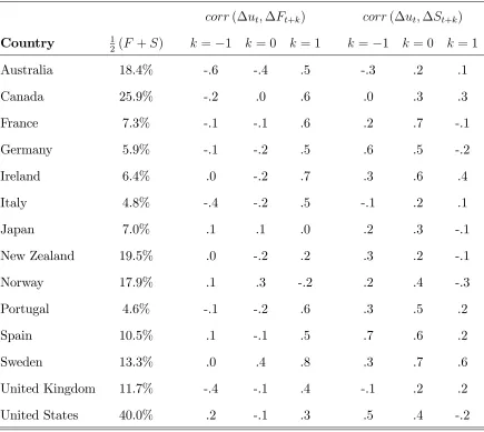
This observation can be seen more formally using a simple correlation analysis. The
last six columns of Table 4 report the contemporaneous, lead, and lag correlations between
the changes in the ‡ows and changes in the unemployment rate. These correlations tell the
following story. In the year prior to a rise in unemployment, in‡ows into the unemployment
pool rise— the one year lead correlation between changes in in‡ows and contemporaneous
changes in unemployment is positive in almost all economies. Moreover, in‡ows remain high
in the year that unemployment rises— the contemporaneous correlation between changes in
in‡ows and changes in unemployment are positive for all countries. In the year following
an unemployment ramp up, out‡ows begin to rise— the one year lag correlation between
changes in out‡ows and contemporaneous changes in unemployment is positive in almost all
economies.
Thus, just like studies that use monthly data for the U.S., we …nd that changes in
in‡ows tend to lead changes in the unemployment rate in the annual data we use. What
emerges from our results on worker ‡ows is that, even though the OECD economies have very
di¤erent levels of ‡ows, the cyclical behavior of worker ‡ows across countries is very similar.
Economic downturns, in which the unemployment rate increases, …rst see an increase in
workers ‡owing into unemployment, rather than a decline in the number of workers ‡owing
out of it. Subsequently, the out‡ows increase as the economy recovers.
These results have stark implications for popular models of the aggregate labor market.
An important recent trend in these models has been to assume that in‡ow rate st into
unemployment is constant over the business cycle (for example Hall, 2005a,b; Blanchard
context of these models, increases in unemployment during recessions are driven entirely by
declines in the job …nding hazard, ft.
This assumption has important implications for the dynamic properties of worker ‡ows
over the cycle. A rich literature on unemployment ‡ows in the U.S. has emphasized that
such models imply that increases in the unemployment rate are preceded by reductions in
the number of workers ‡owing out of the unemployment pool,Ft (Darby, Haltiwanger, and
Plant, 1985, 1986; Blanchard and Diamond, 1990; Davis, 2006). Consequently, reductions
in out‡ows are predicted tolead increases in the unemployment rate in this class of models.
In addition, because the in‡ow ratestis assumed constant, these models also imply that the
number of workers ‡owing into the unemployment pool St will decline modestly in the wake
of a recession as the employment rate 1 ut falls, so that changes in St lag changes in the
unemployment rate. Thus, models that assume a constant in‡ow rate have two important
predictions with regard to worker ‡ows: (i) when unemployment goes up gross worker ‡ows
decline, and (ii) out‡ows lead changes in unemployment, while in‡ows lag.
The studies of worker ‡ows in the U.S. cited above have established that neither of these
theoretical implications is borne out by the data for the U.S. This has led researchers to
challenge the empirical relevance of such models in the U.S. context (Davis, 2006; Fujita and
Ramey, 2009; Ramey, 2008). Our results reveal that the observation of increased in‡ows
as a leading indicator of increased unemployment, far from being unique to U.S. data, is
something close to a stylized fact for all modern developed labor markets.
These results con…rm and reinforce earlier …ndings based on earlier periods for subsets
of the European countries that we study. Using Portuguese microdata from the early 1990s,
Blanchard and Portugal (2001) emphasize that the levels of worker ‡ows are much lower in
Portugal relative to the U.S. Similar …ndings are reported by Bertola and Rogerson (1997,
Table 3) who document reduced worker ‡ows in Italy and Germany relative to Anglo-Saxon
U.K. up to the early 1990s, Balakrishnan and Michelacci (2001) and Burda and Wyplosz
(1994) have highlighted that both in‡ows and out‡ows increased as European unemployment
soared in the 1970s and 1980s, with increased in‡ows leading increased unemployment.
6
Conclusion
Our analysis of publicly available data from the OECD provides four contributions to our
understanding of unemployment ‡ows. First, we present a method of estimating the ‡ow
hazard rates for entering and exiting unemployment across fourteen developed economies,
building on the method pioneered by Shimer (2007) for the U.S. An important bene…t of
this methodology is that it can be extended to estimate unemployment ‡ows for additional
economies over longer time periods as more data becomes available.
Application of this method to fourteen OECD countries uncovers a stark contrast in
av-erage ‡ow hazard rates between Anglo-Saxon, Nordic, and Continental European countries.
Anglo-Saxon and Nordic labor markets are characterized by high unemployment in‡ow and
out‡ow rates, while these ‡ow hazard rates in Continental European economies are generally
less than half of those in their Anglo-Saxon counterparts. Notably, results for the U.S. which
have received much attention in recent literature are a conspicuous outlier among developed
economies, with in‡ow and out‡ow rates that are at least …fty percent larger than the
re-maining economies in our sample. These results strengthen and extend earlier work that has
diagnosed European labor markets as sclerotic based on similar …ndings for subsets of the
economies we study.
Our second contribution is to devise a decomposition of unemployment ‡uctuations into
parts due to changes in in‡ow and out‡ow rates that can be applied to countries with very
di¤erent unemployment dynamics. Conventional decompositions applied to U.S. data have
exploited the fact that unemployment is closely approximated by its steady-state value in
countries outside the U.S., however, we demonstrate that unemployment deviates
consider-ably from its steady-state level. Consequently we show that conventional decompositions
lead to misleading results on the relative importance of ‡uctuations in in‡ow and out‡ow
rates for the dynamics of the unemployment rate. The results from applying our alternative
decomposition reveal approximately a 15:85 in‡ow/out‡ow contribution to unemployment
variation among Anglo-Saxon countries, whereas in most European countries the split is
much closer to 45:55.
Our third contribution is based on a simple correlation analysis of changes in worker
‡ows and changes in the unemployment rate over time. For all countries in our sample,
worker ‡ows tend to increase when unemployment increases. Moreover, we …nd that, in
almost all countries in our sample, changes in in‡ows into unemployment lead changes in
the unemployment rate, while changes in out‡ows tend to lag unemployment variation.
This con…rms and reinforces the conclusions of previous literature based on a smaller set of
countries, suggesting that these …ndings for worker ‡ows are a stylized fact of modern labor
markets.
Stepping back, our empirical …ndings provide an important perspective on the theoretical
literature on unemployment ‡ows that has evolved in recent years. Much of this recent
literature has assumed the in‡ow rate into unemployment to be an exogenous constant. As
a reaction to this, a number of studies of U.S. unemployment ‡ows has cautioned against
this trend (Elsby, Michaels, and Solon, 2009; Fujita and Ramey, 2009; and Yashiv, 2007).
A fourth contribution of the results of this paper is that the same conclusion extends to the
analysis of labor markets in a wide range of developed economies, and especially so if one is
7
References
Albaek, Karsten and Bent E. Sørensen, “Worker Flows and Job Flows in Danish
Manufac-turing, 1980-91,”Economic Journal, 451 (1998), 1750-1771.
Bachmann, Ronald, “Labour Market Dynamics in Germany: Hirings, Separations, and
Job-to-job Transitions over the Business Cycle,” SPB 649 Discussion Paper 2005-045 (2005).
Baker, Michael, “Unemployment Duration: Compositional E¤ects and Cyclical Variability,”
American Economic Review, 82 (1992), 313-21.
Balakrishnan Ravi, and Claudio Michelacci, “Unemployment Dynamics across OECD
Coun-tries,”European Economic Review, 45 (2001), 135-165.
Bauer, Thomas and Stefan Bender, “Technological Change, Organizational Change, and Job
Turnover,”Labour Economics 11 (2004), 265-291.
Bell, Brian and James Smith, “On Gross Flows in the United Kingdom: Evidence from the
Labour Market Survey,” Bank of England Working Paper No.160 (2002).
Bentolila, Samuel, Juan J. Dolado, and Juan F. Jimeno, “Two-tier Employment Protection
Reforms: The Spanish Experience,”Journal for International Comparisons, 6 (2008), 49-56.
Bertola, Giuseppe and Richard Rogerson, “Institutions and Labor Reallocation,”European
Economic Review,41 (1997), 1147-1171.
Blanchard, Olivier and Jordi Gali, “A New Keynesian Model with Unemployment,” MIT
and CREI mimeograph (2006).
Blanchard, Olivier J. and Peter Diamond, “The Cyclical Behavior of the Gross Flows of U.S.
Blanchard, Olivier and Augustin Landier, “The Perverse E¤ects of Partial Labor Market
Reform: Fixed Duration Contracts in France,”Economic Journal, 112 (2002), 214-244.
Blanchard, Olivier J. and Lawrence Summers, “Hysteresis and European Unemployment,”
NBER Macroeconomics Annual (Cambridge, MA: MIT Press, 1986).
Blanchard, Olivier J. and Justin Wolfers, “The Role of Shocks and Institutions In The Rise
of European Unemployment: The Aggregate Evidence,”Economic Journal, 110 (2000), 1-33.
Blanchard, Olivier J. and Pedro Portugal, “What Hides Behind an Unemployment Rate:
Comparing Portuguese and U.S. Labor Markets,”American Economic Review, 91 (2001),
187-207.
Braun, Helge, Reinout de Bock, and Ricardo DiCecio, “Aggregate Shocks and Labor Market
Fluctuations,” Federal Reserve Bank of St. Louis working paper 2006-004 (2006).
Burda, Michael, and Charles Wyplosz, “Gross Worker and Job Flows in Europe,”European
Economic Review, 38 (1994), 1287-1315.
Costain, James, Juan F. Jimeno and Carlos Thomas, “Employment ‡uctuations in a dual
labor market,” Banco de España working paper no. 2013 (2010).
Darby, Michael R., John C. Haltiwanger, and Mark W. Plant, “Unemployment Rate
Dy-namics and Persistent Unemployment under Rational Expectations,”American Economic
Review, 75 (1985), 614-637.
Darby, Michael R., John C. Haltiwanger, and Mark W. Plant, “The Ins and Outs of
Unem-ployment: The Ins Win,”Working Paper No. 1997, National Bureau of Economic Research
(1986).
Davis, Steven J., “Fluctuations in the Pace of Labor Reallocation,”Carnegie-Rochester
Davis, Steven J. “Job Loss, Job Finding, and Unemployment in the U.S. Economy over the
Past Fifty Years: Comment,” in M. Gertler and K. Rogo¤ (Eds.), NBER Macroeconomics
Annual (Cambridge, MA: MIT Press 2006).
Elsby, Michael, Ryan Michaels, and Gary Solon, “The Ins and Outs of Cyclical
Unemploy-ment,”American Economic Journal: Macroeconomics, 1 (2009), 84-110.
Elsby, Michael W. L., Bart Hobijn, and Ay¸segül ¸Sahin, “The Labor Market in the Great
Recession,”Brookings Papers on Economic Activity, (2010), 1–48.
Fujita, Shigeru and Garey Ramey, “The Cyclicality of Job Loss and Hiring,”International
Economic Review, 50 (2009), 415-430.
Gertler, Mark and Antonella Trigari, “Unemployment Fluctuations with Staggered Nash
Wage Bargaining,”Journal of Political Economy 117 (2009), 38-86.
Gomes, Pedro, “Labour Market Flows: Facts from the UK,” London School of Economics
mimeograph (2008).
Hall, Robert E., “Job Loss, Job-…nding, and Unemployment in the U.S. Economy over the
Past Fifty Years,”NBER Macroeconomics Annual (2005a).
Hall, Robert E., “Employment E¢ ciency and Sticky Wages: Evidence from Flows in the
Labor Market,”Review of Economics and Statistics, 87 (2005b), 397-407.
Hobijn, Bart and Ay¸segül ¸Sahin, “Job-Finding and Separation Rates in the OECD,”
Eco-nomics Letters, 104 (2009), 107-111.
Jolivet, Gregory, Fabien Postel-Vinay, Jean-Marc Robin, “The Empirical Content of the Job
Search Model: Labor Mobility and Wage Distributions in Europe and the US,”European
Kaitz, Hyman, “Analyzing the Length of Spells of Unemployment,”Monthly Labor Review, 93 (1970), 11-20.
Kennan, John, “Job Loss, Job Finding, and Unemployment in the U.S. Economy over the
Past Fifty Years: Comment,” in M. Gertler and K. Rogo¤ (Eds.), NBER Macroeconomics
Annual (Cambridge, MA: MIT Press 2006).
Krusell, Per, Toshihiko Mukoyama, and Ay¸segül ¸Sahin, “Labour-Market Matching with
Precautionary Savings and Aggregate Fluctuations,”Review of Economic Studies,77 (2010),
1477-1507.
Machin, Stephen and Alan Manning, “The Causes and Consequences of Longterm
Unem-ployment in Europe,” in O. Ashenfelter and D. Card (Eds.), Handbook of Labor Economics
(Elsevier 1999).
Marston, Stephen T., “Employment Instability and High Unemployment Rates,”Brookings
Papers on Economic Activity, (1976), 169-210.
Merz, Monika, “Heterogeneous Job-matches and the Cyclical Behavior of Labor Turnover,”Journal
of Monetary Economics (1999), 91-124.
Organization for Economic Cooperation and Development (OECD),Employment and Labour
Market Statistics: Labour force status by sex and age, (2010a).
Organization for Economic Cooperation and Development (OECD), Main Economic
Indi-cators, (2010b).
Perry, George L., “Unemployment Flows in the U.S. Labor Market,”Brookings Papers on
Economic Activity, (1972), 245-78.
Petrongolo, Barbara, and Christopher A. Pissarides, “The Ins and Outs of European
Pissarides, Christopher A., “Unemployment and Vacancies in Britain,”Economic Policy, 1 (1986), 499-541.
Pissarides, Christopher A., “The Unemployment Volatility Puzzle: Is Wage Stickiness the
Answer?”Econometrica, 77 (2009), 1339-1369.
Ramey, Garey, “Exogenous vs. Endogenous Separation,” University of California at San
Diego mimeograph (2008).
Reichling, Felix, “Retraining the Unemployed in a Matching Model with
Turbulance,”Stan-ford University mimeograph (2005).
Ridder, Geert and Gerard J. van den Berg, “Measuring Labor Market Frictions: A
Cross-Country Comparison,”Journal of the European Economic Association, 1 (2003), 224-244.
Salant, Stephen W., “Search Theory and Duration Data: A Theory of Sorts,”Quarterly
Journal of Economics, 91 (1977), 39-57.
Shimer, Robert, “The Cyclical Behavior of Equilibrium Unemployment and Vacancies,”
American Economic Review, 95 (2005), 25-49.
Shimer, Robert, “Reassessing the Ins and Outs of Unemployment,” University of Chicago
mimeograph (2007).
Shimer, Robert, “The Probability of Finding a Job,”American Economic Review Papers
and Proceedings, 98 (2008), 268-273.
Yashiv, Eran, “U.S. Labor Market Dynamics Revisited,”Scandinavian Journal of
A
Mathematical details
Estimation of Out‡ow Rates. De…ne the fraction of the labor force that has been
unemployed in month t for less than a month as u1;t, more than one but less than three
months asu3;t, more than three but less than six months asu6;t, more than six but less than
twelve months u12;t, and more than 12 months as u1;t. Then u<1t = u1;t, u<3t =u1;t+u3;t,
etc. Given this data and quarterly data for the unemployment rate, the four estimates of
the out‡ow rate are given by:
ft<1 = ln (u3;t+u6;t+u12;t+u1;t) + 2
3ln (u1;t+u3;t+u6;t+u12;t+u1;t) + 1
3lnut 3, ft<3 = (ln (u6;t+u12;t+u1;t) lnut 3)=3,
ft<6 = (ln (u12;t+u1;t) lnut 6)=6, and
ft<12 = (ln (u1;t) lnut 12)=12. (20)
In practice, we have annualized data for the duration distribution of unemployment, and
we do not know which month(s) of the year the measures refer to. Therefore, our estimates
of the out‡ow rates use averages of the lagged unemployment rates, ut 3, ut 6, and ut 12
over the four quarters in the year for which the out‡ow rate is estimated.
Asymptotic Distribution of Out‡ow Rate Estimates. We do not observe exact
measures of u1;t, u3;t, u6;t, u12;t, and u1;t. Instead we observe their sample approximations
based on labor force survey data for each of the di¤erent countries. Denote the sample size
of the labor force survey by nt, and let bud;t for d 2 f1;3;6;12;1g be the estimated labor
force shares.
In addition, we also observe the estimated unemployment rate but, not only at t but also
atubt 3,ubt 6, andubt 12. We assume that the sample of individuals in the labor force survey