Evaluating Default Policy: The Business Cycle Matters
Supplementary Appendices
Grey Gordon
Indiana University
June 14, 2013
A
Extended Model [For Online Publication]
This appendix contains an extended model description. The objective is to arrive at the simplified definition of equilibrium presented in the main text. The extended model allows for any finite number of z shocks, provided there are a corresponding number of Arrow securities A0z0 with prices ¯qz0(S) and z-contingent contracts with prices qz0(a0z0, s;S).
A.1
The Household Problem
The household problem is the same as in the main text, but with possibly more than two types ofz-contingent contracts.
A.2
The Intermediary’s Problem
The financial intermediary’s problem is to maximize the net present value of financial wealth using contracts, capital, and an aggregate-complete set of Arrow securities. He discounts future wealth using the state-contingent prices ¯qz0(S) of the Arrow securities. It is useful
to think of a contract as a tuple (a0, s, z0) specifying an amounta0, the counterparty to the contract as summarized in s, and the contingency z0 in which the debt (or savings) will be delivered. The intermediary’s contract holdings can be thought of as portfolioslz0 :A⇥S !
R, one for eachz0. It is useful to introduce two functions that aggregate the prices and yields of these portfolios. For any given portfolio of contract holdings m:A⇥S !R, define
C(m;S) := X
a,s
and
Cz00(m;S) :=
1 ¯
qz0(S) X
a0,s
m(a0, s)qz0(a0, s;S)a0. (2)
C(m;S) is the yield of a portfolio of contractsm andCz00(m;S) is the price of those contracts
normalized by ¯qz0(S). This normalization ensures Cz00(·;S) = C(·;Sz00) in equilibrium.
Using these definitions, the intermediary’s problem can be written
P(A, K, l;S) = max
A0
z0,K0 0,l0z0
D+X
z0
¯
qz0(S)P(A0z0, K0, lz00;Sz00)
D+X
z0
¯
qz0(S)Cz00(l0z0;S) + X
z0
¯
qz0(S)A0z0+K0 =C(l;S) +A+ (1 +r(S) )K.
(3)
Let the policy functions for the intermediary be denoted A0z0(A, K, l;S), K0(A, K, l;S), and lz00(A, K, l;S).
A.3
Equilibrium
For now, expand the definition ofS to bez together with a distributionµ(a, e, s, h) of house-holds andl, A, K, N satisfyingK >0,N >0,A= 0, and C(l;S) +A+ (1 +z↵(K/N)↵ 1
)K = 0. A recursive competitive equilibrium is a collection of price functions r, w,q¯z0, qz0,
repayment ratesp, policy functionsc, a0
z0, d, value functionsV, P, and a law of motion such
that all of the following hold:
1. Household policies solve their problem.
2. The financial intermediary’s policies solve his problem.
3. Factor prices are competitive (ensuring the production firm optimizes):
r(S) = z↵(K/N)↵ 1 (4)
w(S) =z(1 ↵)(K/N)↵ (5)
4. Asset and factor markets clear:
N =s edµ (6)
K0(A, K, l;S)>0 (7)
5. Each contract market clears:
lz00(A, K, l;S)(a0, s) + Z
1[a0 =a0z0(a, e, s, h;S)]µ(da, de, s, dh) = 08a0, s, z0 (9)
6. The goods market clears (as ensured by Walras’ law). 7. Repayment probabilities are consistent:
p(a, s 1;S) = X
s
F(s|s 1, z) Z
(1 d(a, e, s,0;S))f(e|s, z)de (10)
for all a0, s,and S (recallS includes z). 8. The intermediary makes zero profits:
C(l0z0;Sz00) +A0z0 + (1 +r(Sz00) )K0 = 0 for each z0 (11) X
z0
¯
qz0(S)Cz00(lz00;S) + X
z0
¯
qz0(S)A0z0 +K0 = 0 (12)
9. The law of motion S0
z0 = (z0,S) is consistent.
A.4
Equilibrium Characterization
In this section I give conditions on the allocations of households that greatly simplify the definition of equilibrium. In particular, if these conditions are met, then there exist prices and optimal policies of the financial intermediary that satisfy market clearing and consistency conditions.
First, I discuss equilibrium pricing.
Lemma 1. The intermediary is indi↵erent over all feasible policies if the no arbitrage con-ditions,
qz0(a0, s;S)a0 = ¯qz0(S)⇢sp(a0, s;Sz00)a0
1 = X
z0
¯
q0z(S)(1 +r(S0
z0) ),
hold.
Proof. If these hold, then the first order conditions for contract holdings, bonds, and capital are satisfied. The first order condition for Arrow securities is trivially satisfied: ¯qz0(S) =
¯
I restrict attention to the prices satisfying the above.
Lemma 2. Equilibrium prices imply C0
z0(lz00;S) = C(lz00;Sz00) for any portfolio l0z0. Further, C0
z0( l0z0;S) = Cz00(lz00;S).
Proof. The first part is proved by
Cz00(lz00;S) :=
1 ¯
qz0(S) X
a0,s
lz00(a0, s;S)qz0(a0, s;S)a0
= 1
¯
qz0(S) X
a0,s
lz00(a0, s;S)¯qz0(S)⇢sp(a0, s;Sz00)a0
=X
a0,s
l0z0(a0, s;Sz00)⇢sp(a0, s;Sz00)a0
=:C(l0z0;Sz00).
The second part is obvious.
Proposition 1. For a given choice of contracts l0
z0, there exist feasible policies K0, A0z0
sat-isfying
K0 >0 and A0z0 = 0
and zero profits if and only if
K0 = C
0
z0( l0z0;S)
1 +r(S0
z0)
>0
for all z0.
Proof. ForA0
z0 = 0, zero profits obtain if and only if X
z0
¯
qz0(S)Cz00(l0z0;S) +K0 = 0 (13)
0 = C(lz00;Sz00) + (1 +r(Sz00) )K0. (14)
Equation (14) is equivalent to
To see this, note
K0 = C(lz00;Sz00)/(1 +r(Sz00) ) (16)
= Cz00(lz00;S)/(1 +r(Sz00) ) (17)
=Cz00( lz00;S)/(1 +r(Sz00) ) (18)
by application of Lemma 2twice.
Because the K0 in (15) is equivalent to (14) by Lemma 2, zero profits will obtain so long as (13) holds. That it holds is proven by
K0 = X
z0
¯
qz0(S)Cz00(lz00;S) (19)
=X
z0
¯
qz0(S)Cz00( lz00;S) (20)
=X
z0
¯
qz0(S)K0(1 +r(Sz00) ) (21)
=K0 (22)
where the last equation follows from the no arbitrage condition in Lemma 1.
Proposition 2. Define µ0
z0 analagously to l0z0 by
µ0z0(a0, s;S) := Z
a,e,h
1[a0 =a0z0(a, e, s, h;S)]µ(da, de, s, dh)
so that µ0z0(a0, s;S) is the measure of households choosing contract (a0, s, z0). If allocations
satisfy
C0
z0(µ0z0;S)
1 +r(S0
z0)
= Cz0˜0(µ0z˜0;S) 1 +r(S0
˜ z0)
>0
for all z0,z˜0 and if prices satisfy
qz0(a0, s;S)a0 = ¯qz0(S)⇢sp(a0, s;Sz00)a0
1 = X
z0
¯
qz0(S)(1 +r(Sz00) )
then there exist optimal policies of the financial intermediary that satisfy zero profit conditions and clear Arrow security, capital, and contract markets. Further, the unique K0 has K0 =
C0
z0(µ0z0;S)/(1 +r(Sz00) ) (for either z0).
indi↵erent over all feasible allocations. Second, specifiying l0
z0 = µ0z0 for the intermediary
clears contract markets. For this choice of l0
z0, by Proposition 1 there exists feasible policies K0 >0, A0
z0 = 0 that satisfy zero profits. Moreover, by Proposition 1, K0 =Cz00(µ0z0;S)/(1 + r(S0
z0) ) for either z0. These policies are feasible, and hence optimal, and clear the capital,
Arrow security, and contract markets.
Proposition 3. Today’s capital stock K can be found in equilibrium from the joint distri-bution µ as the unique K solving
(1 +r(S) )K =
Z
a(1 d(a, e, s, h;S))dµ
where r(S) =z↵(K/N)↵ 1 and w(S) =z(1 ↵)(K/N)↵ (and N =R edµ).
Proof. First, define
˜
p(a, s;S) :=
Z
(1 d(a, e, s,0;S))f(e|s, z)de
so that p(a0, s;S0
z0) = P
s0F(s0|s, z0)˜p(a0, s0;Sz00). Now, note that zero-profits and Arrow
se-curity market clearing imply (1 +r(S0
z0) )K0 = C(lz00;Sz00). From this,
(1 +r(Sz00) )K0
=X
a0,s
lz00(a0, s)⇢sp(a0, s;Sz00)a0 (23)
=X
a0,s
(X
a,h Z
1[a0 =a0(a, e, s, h;S)]µ(a, de, s, h))⇢sp(a0, s;S0
z0)a0 (24)
=X
a0 X
a,s,h
p(a0, s;Sz00)a0 Z
⇢s1[a0 =a0(a, e, s, h;S)]µ(a, de, s, h) (25)
=X a0 X a,s,h (X s0
F(s0|s, z0)˜p(a0, s0;Sz00))a0 Z
⇢s1[a0 =a0(a, e, s, h;S)]µ(a, de, s, h) (26)
=X
a0,s0
˜
p(a0, s0;S0
z0) X
a,s,h
F(s0|s, z0)a0 Z
⇢s1[a0 =a0(a, e, s, h;S)]µ(a, de, s, h) (27)
=X
a0,s0
˜
p(a0, s0;Sz00)a0 Z
⇢sF(s0|s, z0)1[a0 =a0(a, e, s, h;S)]dµ(a, e, s, h) (28)
where (23) uses the definition ofC(·), (24) uses contract market clearing, (25) just rearranges, (26) uses the definition of p and ˜p, and (27)-(28) rearrange again. Now because households are born with zero assets, a0µ
a0, s0, z0 where I’ve usedµ
z0 to denote the distribution implicit in Sz00. Using this fact,
(1 +r(Sz00) )K0 (29)
=X
a0,s0
˜
p(a0, s0;Sz00)a0µz0(a0, s0) (30)
=X
a0,s0
˜
p(a0, s0;Sz00)a0 X
h0
µz0(a0, s0, h0) (31)
= X
a0,s0,h0
˜
p(a0, s0;S0
z0)a0µz0(a0, s0, h0) (32)
=
Z
(1 d(a0, e0, s0,0;Sz00))a0dµz0(a0, e0, s0, h0) (33)
where (30) substitutes, (31) uses a probability measure property, (32) rearranges, and (33) uses the definition of ˜pand the property µz0(a0, e0, s0, h0) =f(e0|s0, z0)µ(a0, s0, h0) (by a law of
large numbers).
I also claim K is unique. This is clear once one notices rK(= ↵Y) is increasing in K.
Using the preceding characterizations, the simplified definition of equilibrium in the main text is readily obtained.
B
Calibration [For Online Publication]
This appendix contains both the data description and additional calibration details.
B.1
Data
The model was constructed to capture the salient features of Chapter 7 bankruptcy in the U.S. Figure 1 shows the annual percent of Chapter 7 filings per household from the period 1960 to 2012.1 The number of households taking advantage of this bankruptcy provision has
drastically increased since 1984 and in 2005 experienced a sharp increase, then decrease, and subsequent recovery. The sharp increase is presumably due to anticipation of the 2005 reform (which mostly applied to filings made on or after October 17, 2005).2 Unfortunately, the
1The data that go back to 1960 are only available on a fiscal year basis ending in June (the series ending
in December 1990). These are available at the Department of Justice website http://www.uscourts.gov/
Statistics/BankruptcyStatistics.aspx#calendar in various pdf files. To recover the annual figure for
yeary prior to 1990, I use the average ofy andy+ 1. To test how well this works, I compare this method’s
values with the known values for the period 1990-2004. This produces a good fit with anR2 of .985.
1960 1965 1970 1975 1980 1985 1990 1995 2000 2005 2010 0.4
0.6 0.8 1 1.2 1.4
Year
% of Hhs Filing
Percent of Households Filing
Figure 1: Chapter 7 Filings Per Household (1960-2012)
sample period drastically a↵ects not only the level of bankruptcies but also their cyclicality and volatility. Because of this, I report statistics for each of the subperiods 1960-1984, 1984-2004, 1997-1984-2004, and 1960-2004. In addition to 1984 and 2005 being breakpoints visually, these were years of substantial bankruptcy reform.3 The period 1997-2004 is considered as
filings appear to level o↵ at the start of this period.
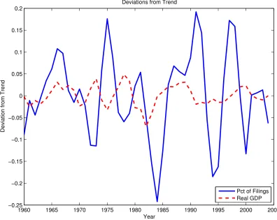
Figure 2 plots log filings per household and log real GDP using the HP filter with pa-rameter 100 for the sample 1960-2004. Visually bankruptcy filings are much more volatile than output and appear to be countercyclical, but not strongly. The weak countercylicality is driven by the the years surrounding 1984 when filings begin a secular increase and the Bankruptcy Amendment Act of 1984 is introduced. This is borne out by the statistics
re-3There were essentially two rounds of substantial bankruptcy legislation. The first round began with the
Marquette decision in 1979 which was subsequently amended by the Bankruptcy Amendment Act of 1984. The second round began with the “Bankruptcy Reform Act of 1999” which was passed by Congress but not signed into law. Subsequent revisions of this legislation resulted in the “Bankruptcy Abuse Prevention and Consumer Protection Act” (BAPCPA) which was signed into law in 2005. Several possible explanations for
1960 1965 1970 1975 1980 1985 1990 1995 2000 2005 −0.25
−0.2 −0.15 −0.1 −0.05 0 0.05 0.1 0.15 0.2
Year
Deviation from Trend
Deviations from Trend
Pct of Filings Real GDP
Figure 2: Cyclical Properties of Filings (1960-2004)
Statistic 1960-2004 1960-1984 1997-2004 1984-2004
Corr(Defaulting Pop,Output) -.03 -.45 -.94 -.02
Stdev(Defaulting Pop) in % 10.25 7.53 8.22 11.07
Stdev(Output) in % 2.44 2.65 1.21 1.58
Stdev(Defaulting Pop)/Stdev(Output) 4.20 2.84 6.79 6.99
Mean(Defaulting Pop*) in % .45 .25 .95 .68
*In levels.
Table 1: Cyclical Properties of Chapter 7 Filings per Household
ported in Table1. Bankruptcy filings are between 2.8 and 7.0 times more volatile than output and are acyclical to countercyclical with a correlation between -.02 and -.94 depending on the sample period.
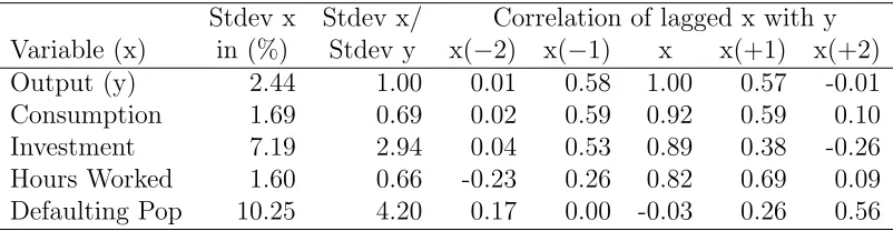
data in Table 2.4 Consumption, investment, and hours worked are all strongly procyclical.
Investment and the fraction of households filing are both much more volatile than output while consumption and hours worked are somewhat less so.
Stdev x Stdev x/ Correlation of lagged x with y Variable (x) in (%) Stdev y x( 2) x( 1) x x(+1) x(+2)
Output (y) 2.44 1.00 0.01 0.58 1.00 0.57 -0.01
Consumption 1.69 0.69 0.02 0.59 0.92 0.59 0.10
Investment 7.19 2.94 0.04 0.53 0.89 0.38 -0.26
Hours Worked 1.60 0.66 -0.23 0.26 0.82 0.69 0.09
Defaulting Pop 10.25 4.20 0.17 0.00 -0.03 0.26 0.56
Table 2: U.S. Business Cycle Properties (1960-2004)
B.2
Calibration
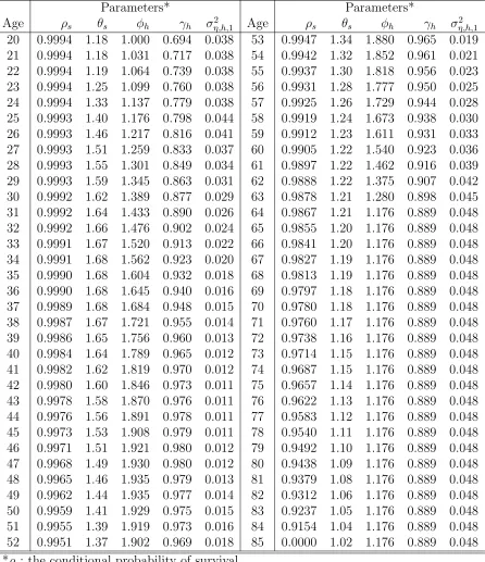
There are several calibration details omitted in the main text. This section fills out the details. Table 3lists the profiles of all variables.
One omitted detail is how the sample in Karahan and Ozkan (2011) of ages 24 to 60 was dealt with. To obtain the shock persistences for younger and older households I assume the cubic profile is correct. To obtain the standard deviations, I assume the profile is correct for older households, but use a di↵erent approach for younger households. Specifically, I assume the standard deviation is constant for younger households and choose it so that the unconditional standard deviation at age 24 is the same as what Karahan and Ozkan (2011) find.
Another detail is how the earnings profile was constructed from the estimates ofHubbard,
Skinner, and Zeldes(1994).Hubbard et al.(1994) estimate separate deterministic profiles for
household heads with less than 12 years of education (NHS), 12-15 years (HS), and 16+ years (COL) of education. I average the profiles of these three types for the year 1986 assuming 13% of the population is NHS, 48% is HS, and 39% is COL. This breakdown of educational attainment is from the 2010 Current Population Survey for ages 30-34.5
4I followOhanian and Ra↵o(2011) and take annual hours worked from the Conference Board’s Total
Econ-omy Database (TED) available at http://www.conference-board.org/data/economydatabase/#files.
Output, consumption, and investment are taken from NIPA as real gross domestic product, real personal consumption expenditures, and real gross private domestic investment. The number of households (used to compute the fraction of households defaulting) is taken from the Census Bureau’s historical tables available athttp://www.census.gov/population/www/socdemo/hh-fam.html#ht(Table HH-1). The number of fil-ings is taken from the Department of Justice website as already described. All variables have been logged and detrended using the HP filter with parameter 100.
Lastly, the consumption equivalence profile was constructed assuming ✓s =f(Ns) where
Ns is the average number of household members (the profile of which was provided to me by
Alexander Bick) and f is the mean equivalence scale in Fern´andez-Villaverde and Krueger
(2007) linearly-interpolated to be continuous. This leads to a consumption equivalence profile very similar to the one in Livshits, MacGee, and Tertilt (2007).
C
Computation [For Online Publication]
The steady state model is computed using a collection of standard techniques. The efficiency process is discretized using the method ofTauchen(1986). The persistent shock is discretized with 30 points with a coverage of ±5 “average unconditional standard deviations in reces-sions,” ¯⌘,b/
p
1 ⇢¯2. The bar denotes the numerical average across ages. The transitory
shock is discretized with 5 points with a coverage of ±5 standard deviations. The right-tail process was discretized with 10 log-spaced points. The mass on each point is computed using, again, the method of Tauchen (1986) (e.g. the mass on the low point is the cdf evaluated at the midpoint of the lowest two points). The asset grid (which is really the knots of the linear interpolant) is comprised of 250 points with 100 strictly negative. These are unevenly spaced and concentrated close to zero. The household problem is solved using backward induction with linear splines (interpolants) representing continuation utilities and expenditure sched-ules. A grid search is first employed to avoid local minima, followed by a one-dimensional version of the simplex method.
The model with aggregate uncertainty is computed using the method of Krusell and
Smith (1998). The “moments” used are the capital-labor ratio and a parameter controlling
the equity premium.6 The equity premiumW is defined on the domain [0,1] and controls ¯q
g
and ¯qb as follows:
¯
qg(S) = ✓
R(G) + W
1 W
F(b|z)
F(g|z)R(B)
◆ 1
and (34)
¯
qb(S) = ✓
(1 W)
W
F(g|z)
F(b|z)R(G) +R(B)
◆ 1
(35)
where R(S) is defined as the return to capital net of depreciation, i.e. R(S) = 1 +r(S) . The probabilities ensure the equilibrium value of W is always close to, but slightly above,
.5. The household problem is solved with backward induction. Linear interpolation is used
6The use of the capital-labor ratio rather than capital and labor separately significantly reduces the
difficulty of the problem and reduces error from highly unlikely states (e.g. very low capital, very high labor)
being included in household expectations. Including an equity premium as a state variable is fairly common in
Parameters* Parameters*
Age ⇢s ✓s h h 2⌘,h,1 Age ⇢s ✓s h h ⌘2,h,1
20 0.9994 1.18 1.000 0.694 0.038 53 0.9947 1.34 1.880 0.965 0.019 21 0.9994 1.18 1.031 0.717 0.038 54 0.9942 1.32 1.852 0.961 0.021 22 0.9994 1.19 1.064 0.739 0.038 55 0.9937 1.30 1.818 0.956 0.023 23 0.9994 1.25 1.099 0.760 0.038 56 0.9931 1.28 1.777 0.950 0.025 24 0.9994 1.33 1.137 0.779 0.038 57 0.9925 1.26 1.729 0.944 0.028 25 0.9993 1.40 1.176 0.798 0.044 58 0.9919 1.24 1.673 0.938 0.030 26 0.9993 1.46 1.217 0.816 0.041 59 0.9912 1.23 1.611 0.931 0.033 27 0.9993 1.51 1.259 0.833 0.037 60 0.9905 1.22 1.540 0.923 0.036 28 0.9993 1.55 1.301 0.849 0.034 61 0.9897 1.22 1.462 0.916 0.039 29 0.9993 1.59 1.345 0.863 0.031 62 0.9888 1.22 1.375 0.907 0.042 30 0.9992 1.62 1.389 0.877 0.029 63 0.9878 1.21 1.280 0.898 0.045 31 0.9992 1.64 1.433 0.890 0.026 64 0.9867 1.21 1.176 0.889 0.048 32 0.9992 1.66 1.476 0.902 0.024 65 0.9855 1.20 1.176 0.889 0.048 33 0.9991 1.67 1.520 0.913 0.022 66 0.9841 1.20 1.176 0.889 0.048 34 0.9991 1.68 1.562 0.923 0.020 67 0.9827 1.19 1.176 0.889 0.048 35 0.9990 1.68 1.604 0.932 0.018 68 0.9813 1.19 1.176 0.889 0.048 36 0.9990 1.68 1.645 0.940 0.016 69 0.9797 1.18 1.176 0.889 0.048 37 0.9989 1.68 1.684 0.948 0.015 70 0.9780 1.18 1.176 0.889 0.048 38 0.9987 1.67 1.721 0.955 0.014 71 0.9760 1.17 1.176 0.889 0.048 39 0.9986 1.65 1.756 0.960 0.013 72 0.9738 1.16 1.176 0.889 0.048 40 0.9984 1.64 1.789 0.965 0.012 73 0.9714 1.15 1.176 0.889 0.048 41 0.9982 1.62 1.819 0.970 0.012 74 0.9687 1.15 1.176 0.889 0.048 42 0.9980 1.60 1.846 0.973 0.011 75 0.9657 1.14 1.176 0.889 0.048 43 0.9978 1.58 1.870 0.976 0.011 76 0.9622 1.13 1.176 0.889 0.048 44 0.9976 1.56 1.891 0.978 0.011 77 0.9583 1.12 1.176 0.889 0.048 45 0.9973 1.53 1.908 0.979 0.011 78 0.9540 1.11 1.176 0.889 0.048 46 0.9971 1.51 1.921 0.980 0.012 79 0.9492 1.10 1.176 0.889 0.048 47 0.9968 1.49 1.930 0.980 0.012 80 0.9438 1.09 1.176 0.889 0.048 48 0.9965 1.46 1.935 0.979 0.013 81 0.9379 1.08 1.176 0.889 0.048 49 0.9962 1.44 1.935 0.977 0.014 82 0.9312 1.06 1.176 0.889 0.048 50 0.9959 1.41 1.929 0.975 0.015 83 0.9237 1.05 1.176 0.889 0.048 51 0.9955 1.39 1.919 0.973 0.016 84 0.9154 1.04 1.176 0.889 0.048 52 0.9951 1.37 1.902 0.969 0.018 85 0.0000 1.02 1.176 0.889 0.048 *⇢s: the conditional probability of survival.
✓s: adult-equivalent household size.
h: deterministic earnings profile. h: income shock persistence. 2
⌘,h,1: persistent shock variance.
to interpolate between aggregate moments (as well as in the household problem). To op-timize, a grid search is used followed by a simplex algorithm (either one-dimensional or two-dimensional depending on the portfolio restrictions). For results to be comparable be-tween the steady state and business cycle versions, the same number and placement of grid points are used in both models (in both the asset and efficiency direction). The model is simulated non-stochastically as in Young (2010), and the asset markets are cleared in each period of the simulation.
The laws of motion take the following form:
" K0/N0
W0
#
=
"
11,zz0 12,zz0 0 21,zz0 22,zz0 0
#2 6 4
1
K/N W
3 7
5 (36)
Here the subscript zz0 means the coefficients are z and z0-dependent. Importantly, W does not influence the one-step ahead forecast. This allows the equity premium to vary holding fixed all other prices. The resulting laws of motion are very accurate for both the experiments in the main paper and the robustness tests.
Because the computational burden is heavy, especially in terms of memory usage, the number of points used for the aggregate moments is kept to a minimum: 5 in the K/N
direction linearly-spaced within ±15% of the steady-state value and 3 in the W direction placed at .50 and .52. Because the natural borrowing limit and welfare depend on the worst possible scenario that can occur, and on how quickly it can be reached, the bounds and the number of grid points used can influence the results. In fact, the grids appear to have a fairly large e↵ect (see the explanation regarding Table 4). The bounds I’ve chosen I believe are reasonable, especially given past U.S. history where the capital-output ratio declined by some 20% in the Great Depression and even since 1960 hours worked per household has seen declines of 4% (relative to trend).7
The model is simulated non-stochastically as in Young(2010). The economy is simulated for 1000 periods and the first 250 periods are discarded. At each point in the simulation, the bond market must be cleared. Because the equity premium is included in the aggregate state space, this is a simple matter of linearly interpolating the asset policies to find an equilibrium
W.
When calculating welfare gains for di↵erent groups, I assume the policy is changedafter households have made their default decisions but before they have made their savings
deci-7Author’s calculations. Hours worked per household are calculated as discussed in Appendix B. The
sions. The timing convention, fromChatterjee and Gordon(2012), ensures no unanticipated losses or gains are inflicted on the intermediary. For the no aggregate risk version, the welfare gains are straightforward to calculate. Defining
!(a, e, s, h) =
✓
VN D(a, e, s, h = 0)
VCD(a, e, s, h)
◆1/(1 )
1,
the population in favor is
Z
((1 d(a, e, s, h))1[!(a, e, s, h)>0] +d(a, e, s, h)1[!(0, e, s,0)>0])dµ
whereµis the steady state distribution from the CD economy. The welfare gain for a subset
I of the population is calculated as
Z
I
((1 d(a, e, s, h))!(a, e, s, h) +d(a, e, s, h)!(0, e, s,0))dµ /µ(I).
Welfare computations in the business cycle are much more difficult to handle. Because the mapping from aggregate moments to distributions is not one-to-one, calculating welfare for households who are not newborn—and hence for whom the joint distribution over wealth, efficiency, and credit history is not known—is not straightforward. To get a rough idea of the changes in welfare, I do the following. First, I define
˜
VX(a, e, s, h) = X
z,m
F(z)⇧X(m|z)VX(a, e, s, h;z, m)
where ⇧X(m|z) is the invariant distribution over aggregate moments from the Krusell and
Smith(1998) method. Consequently, ˜VX is an “average” value function in economyX. I then
define
˜
d(a, e, s, h) = max
z,m d(a, e, s, h;z, m).
Lastly, I define
˜
!(a, e, s, h) = V˜N D(a, e, s, h = 0) ˜
VCD(a, e, s, h)
!1/(1 )
1.
The population in favor is
Z ⇣
(1 d˜(a, e, s, h))1[!(a, e, s, h)>0] + ˜d(a, e, s, h)1[!(0, e, s,0)>0]⌘dµ
gain for a subset I of the population is
Z
I ⇣
(1 d˜(a, e, s, h))˜!(a, e, s, h) + ˜d(a, e, s, h)˜!(0, e, s,0)⌘dµ /µ(I)
These aggregate risk welfare measures are rather crude. Ideally one would store the entire distribution and value function across a long simulated series, compute the gain, and then average the gain. Unfortunately, because of the memory requirements involved in that ap-proach, it is not really practical. An alternative approach would be to use the method of
Gordon (2011) to keep the distribution as a state-variable. However, for the large
distribu-tion used in this paper, this approach would also require substantial computadistribu-tion power. The ex-ante measure of newborn welfare is free from this problem as it does not require a distribution to calculate it.
D
Robustness [For Online Publication]
This section conducts robustness tests. The focus is on the consequences of eliminating default rather than restricting it.
D.1
Components of the Business Cycle
One of the key results is that business cycles reduce the welfare gain of eliminating default. However, business cycles in the model have three components: a TFP shockz, an aggregate labor supply shifter (LSS) z, and counter-cyclical earnings variance (CEV) of the persistent earnings shock ⌘,h,z. I now examine how each of these contribute to the total reduction in
the welfare gain of eliminating default.
I proceed by starting with all three components (the benchmark) and eliminating them successively until the model is equivalent to the steady state one. I eliminate elements in the following order: CEV, LSS, and TFP. The last step results in a “steady state.” However, because the grids for K/N andW (W is an equity premium, see Appendix C) are the same as in the business cycle version, these numbers di↵er from the usual “steady state” measure (where the “grids” are measure zero, specifically KSS/NSS and WSS). For ease of reference,
I also report this usual steady environment and label it “SS.”
components eliminated but also has aggregate moment grids of zero measure. This results in a welfare gain of 3.78%.
Eliminating, left to right
Nothing CEV LSS TFP SS
Welfare Gain (%) 2.73 2.65 2.30 2.82 3.78 Population in Favor (%) 63.4 62.9 61.8 62.0 60.4
Table 4: Contribution of Business Cycle Components to Welfare Results
When considering how the natural borrowing limit works, this is not very surprising. All that matters is that there exist a positive probability of a state being realized in order for it to have an e↵ect. By having interpolation and non-zero measure grids, the computation e↵ectively causes this. This in fact demonstrates how fragile a natural borrowing limit econ-omy is. Even without adding shocks, just changing the support of the grids can have a large e↵ect. Because of this it is important to have reasonable grids; Appendix C which discusses the grids argues they are reasonable.
D.2
Guaranteed Earnings Prior to Retirement
In the paper, it was argued that using a low minimum value for earnings during working life is reasonable. I now explore the robustness of the results to guaranteed earnings prior to retirement.
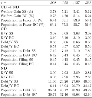
To provide guaranteed earnings, I do the following. Given the efficiency distribution of the benchmark economy, I replace any values less than a threshold⌧ with⌧ and re-normalize so that N = 1 in steady state. I consider 4 di↵erent thresholds ⌧ 2 {.008, .058, .127, .233}. These represent a lower bound of roughly $500, $3500, $7,600, and $14,000 taking average household labor income to be $60,000 and are the values considered inAthreya (2008). The benchmark is any value of⌧ .011.
Table5reports the results. With the exception of⌧ =.233, the welfare gain of eliminating default falls when aggregate risk is added. Also, in general the fall is larger the smaller ⌧
is. Also, the CD economy looks virtually the same regardless of ⌧ while the ND economy becomes increasingly indebted as ⌧ increases.
⌧ = .008 .058 .127 .233
CD ! ND
Welfare Gain SS (%) 3.78 5.21 5.41 5.12 Welfare Gain BC (%) 2.73 4.70 5.14 5.24 Population in Favor SS (%) 60.4 55.1 53.9 50.1 Population in Favor BC (%) 63.4 57.5 55.7 51.6
CD
K/Y SS 3.08 3.08 3.08 3.08
K/Y BC 3.10 3.10 3.10 3.09
Debt/Y SS 0.66 0.66 0.66 0.68
Debt/Y BC 0.57 0.57 0.57 0.59
Population in Debt SS 7.12 7.12 7.10 7.89 Population in Debt BC 6.42 6.43 6.45 7.35 Population Filing SS 0.45 0.45 0.45 0.45 Population Filing BC 0.44 0.45 0.45 0.45
ND
K/Y SS 3.00 2.92 2.89 2.81
K/Y BC 3.05 2.98 2.95 2.86
Debt/Y SS 11.06 23.20 27.09 40.30
Debt/Y BC 6.11 15.94 20.79 34.47
Population in Debt SS 35.61 40.12 40.99 43.27 Population in Debt BC 30.74 37.46 39.08 42.10
Table 5: Robustness to Guaranteed Income
Overall, these results suggest that, to the extent earnings are guaranteed in working life, it would be substantially welfare improving to eliminate default. However, the gain would be overstated if aggregate risk was not accounted for except in cases where a very large amount of earnings are guaranteed.
D.3
Retirement Schemes
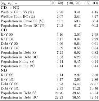
In the benchmark calibration, labor income in retirement is comprised of a guaranteed frac-tion G=.15 of average earnings and a fractionF =.35 of earnings from the last period of working life. The average replacement rate is roughly 50% because G+F =.5. However, as already discussed, it is not the replacement rate that really matters but how much of it is guaranteed. I now examine the robustness of the results to alternative replacement schemes (G,F) subject to keeping G+F =.5.
(G,F) = (.00, .50) (.30, .20) (.50, .00)
CD !ND
Welfare Gain SS (%) 2.28 3.41 4.15
Welfare Gain BC (%) 2.07 2.84 3.47
Population in Favor SS (%) 68.7 59.4 56.4 Population in Favor BC (%) 70.3 61.7 60.2
CD
K/Y SS 3.16 3.03 2.98
K/Y BC 3.17 3.04 2.99
Debt/Y SS 0.66 0.64 0.61
Debt/Y BC 0.59 0.56 0.54
Population in Debt SS 7.25 6.92 6.82
Population in Debt BC 6.53 6.25 6.01
Population Filing SS 0.44 0.45 0.44
Population Filing BC 0.44 0.45 0.44
ND
K/Y SS 3.14 2.92 2.80
K/Y BC 3.17 2.96 2.86
Debt/Y SS 3.23 15.43 27.67
Debt/Y BC 2.35 11.21 19.76
Population in Debt SS 24.70 39.65 45.53 Population in Debt BC 22.23 36.55 42.54
Table 6: Robustness of Results to Alternative Retirement Schemes
earnings are guaranteed. These results agree with the argument developed in the paper: a large amount of guaranteed retirement earnings results in a large natural borrowing limit that is substantially a↵ected by fluctuating factor prices.
D.4
Profiles
Many of the parameters in the model are age-dependent. In particular, there are profiles for survival probabilities ⇢s, adult-equivalent household size ✓s, deterministic earnings h,
income persistence h, and persistent shock variance ⌘2,h,z. While these bring the model
closer in line with the data, they also make interpreting the results more difficult. I examine the consequences of these profiles by separately setting⇢s,✓s,and h to 1 and also by setting h, ⌘2,h,z, and 2" to the age-independent estimates inStoresletten, Telmer, and Yaron(2004)
(STY).8
Table 7 reports the results. In each of these tests, aggregate risk reduces the benefit of
8The STY estimates I use are
h=.952, ⌘,h,g =.125, ⌘,h,b =.211, and "=.255 for allh. As in the
h, ⌘,h,z, ",h ⇢s= 1 ✓s= 1 h = 1 = STY est.
CD ! ND
Welfare Gain SS (%) 4.78 5.56 1.06 2.62
Welfare Gain BC (%) 3.25 3.90 0.88 2.00
Population in Favor SS (%) 54.1 58.6 58.3 66.5 Population in Favor BC (%) 57.3 62.0 60.9 68.8
CD
K/Y SS 3.22 3.21 3.04 3.13
K/Y BC 3.23 3.22 3.06 3.15
Debt/Y SS 0.73 0.75 0.24 0.56
Debt/Y BC 0.63 0.65 0.21 0.49
Population in Debt SS 7.43 8.79 3.60 4.87
Population in Debt BC 6.68 7.66 3.05 4.49
Population Filing SS 0.39 0.46 0.21 0.46
Population Filing BC 0.43 0.46 0.21 0.48
ND
K/Y SS 3.10 3.11 2.96 3.08
K/Y BC 3.17 3.17 3.00 3.12
Debt/Y SS 16.13 13.76 7.86 5.37
Debt/Y BC 8.11 7.34 5.27 3.43
Population in Debt SS 36.08 36.32 28.91 28.85 Population in Debt BC 31.30 32.07 24.51 24.31
Table 7: Robustness of Results to Flat Profiles
eliminating default. The h = 1 case is worth pointing out because it is indicative of what
results from an infinite-horizon economy might look like: because households do not have life-cycle reasons to borrow, credit and default are less important. Overall, the results look about the same both in terms of welfare and allocations.
D.5
Flexible Portfolios
In the calibrated model, most households are restricted to use portfolios that just replicate a risk-free bond,a0
g =a0b. I now relax this assumption, and, in particular, allow every household
to choose any portfolio, i.e. to choose a0
g independently of a0b.
Flexible Benchmark
CD! ND
Welfare Gain SS (%) 3.78 3.78
Welfare Gain BC (%) 2.96 2.73
Population in Favor SS (%) 60.4 60.4 Population in Favor BC (%) 62.8 63.4
CD
K/Y SS 3.08 3.08
K/Y BC 3.10 3.10
Debt/Y SS 0.66 0.66
Debt/Y BC 0.63 0.57
Population in Debt SS 7.12 7.12
Population in Debt BC 7.09 6.43
Population Filing SS 0.45 0.45
Population Filing BC 0.46 0.45
ND
K/Y SS 3.00 3.00
K/Y BC 3.04 3.05
Debt/Y SS 11.06 11.06
Debt/Y BC 7.49 6.11
Population in Debt SS 35.61 35.61
Population in Debt BC 32.47 30.74
Table 8: Robustness of Results to Flexible Portfolios
References
K. B. Athreya. Default, insurance and debt over the life-cycle. Journal of Monetary Eco-nomics, 55(4):752–774, 2008.
S. Chatterjee and G. Gordon. Dealing with consumer default: Bankruptcy vs garnishment. Journal of Monetary Economics, 59(S):S1–S16, 2012.
J. Fern´andez-Villaverde and D. Krueger. Consumption over the life cycle: Facts from the consumer expenditure survey data. The Review of Economics and Statistics, 89(3):552– 565, 2007.
G. Gordon. Computing dynamic heterogeneous-agent economies: Tracking the distribution. PIER Working Paper 11-018, University of Pennsylvania, 2011.
F. Karahan and S. Ozkan. On the persistence of income shocks over the life cycle: Evidence and implications. PIER Working Paper 11-030, University of Pennsylvania, 2011.
P. Krusell and A. A. Smith, Jr. Income and wealth heterogeneity in the macroeconomy. Journal of Political Economy, 106(5):867–896, 1998.
I. Livshits, J. MacGee, and M. Tertilt. Consumer bankruptcy: a fresh start. American Economic Review, 97(1):402–418, 2007.
I. Livshits, J. MacGee, and M. Tertilt. Accounting for the rise in consumer bankruptcies. American Economic Journal: Macroeconomics, 2(2):165–93, 2010.
L. Ohanian and A. Ra↵o. Hours worked over the business cycle in OECD countries, 1960-2010. Mimeo, 2011.
K. Storesletten, C. Telmer, and A. Yaron. Cyclical dynamics in idiosyncratic labor market risk. Journal of Political Economy, 112(3):695–717, 2004.
K. Storesletten, C. Telmer, and A. Yaron. Asset pricing with idiosyncratic risk and overlap-ping generations. Review of Economic Dynamics, 10(4):519–548, October 2007.
G. Tauchen. Finite state markov-chain approximations to univariate and vector autoregres-sions. Economics Letters, 20(2):177–181, 1986.