Dynamics of Investment, Debt, and Default
∗
Grey Gordon
†Pablo A. Guerron-Quintana
‡April 18, 2017
Abstract
This paper proposes a sovereign default model with long-term debt and endogenous output and investment that simultaneously accounts for default episodes and business cycles in emerging economies. In response to positive productivity shocks, risk pre-mia fall and the sovereign borrows to finance investment. When adverse productivity shocks make international borrowing expensive, the sovereign responds by rolling over debt and reducing investment. This causes output to fall and the debt-output ratio to increase, and default occurs if the negative shocks continue long enough. Consequently, the model generates first an increase and then a decrease in investment, consumption, and output prior to default, as in the data. These relationships between productivity, spreads, investment, and borrowing also make the model consistent with many features of small open economy business cycles such as countercyclical spreads and net exports. While capital has non-trivial effects on the incentive to default, increased capital almost always reduces risk premia in equilibrium.
Keywords: Investment, Debt, Default, Long-Term Debt
JEL classification numbers: F34, F41, F44
∗We thank Roc Armenter, Yan Bai, Satyajit Chatterjee, Burcu Eyigungor, Joao Gomes, Juan Carlos
Hatchondo, Urban Jermann, Diogo Lima, Leo Martinez, Makoto Nakajima, Jim Nason, and seminar par-ticipants at the University of Kyoto, Federal Reserve Bank of Philadelphia, Wharton, and the NYU/FRBA International Conference for their valuable comments. Joy Zhu provided superb research assistance. This research was supported in part by Lilly Endowment, Inc., through its support for the Indiana University Pervasive Technology Institute, and in part by the Indiana METACyt Initiative. The Indiana METACyt Initiative at IU is also supported in part by Lilly Endowment, Inc.
1
Introduction
Defaults are a pervasive feature of emerging economies. Among countries who have defaulted
at least once, the annual default rate from 1980 to 2012 was 3.8% (Tomz and Wright, 2013,
p. 257). Moreover, defaults are becoming more prevalent over time: The number of defaults
and reschedules in Latin America and Asia was nearly three times larger in 1975-2006 than in
1950-1974 (Reinhart and Rogoff,2008, p. 27). Hence, to properly understand business cycles
in emerging economies, one must account for the joint dynamics of output, consumption, investment, net exports, and interest rates in and around sovereign defaults.
In this paper, we propose and analyze a sovereign default model with endogenous
cap-ital accumulation that simultaneously accounts for empirical features of sovereign default
episodes and business cycle properties of small open economies. With respect to default
episodes, the model captures the data’s boom, bust, and recovery pattern around defaults
both qualitatively and quantitatively. For instance, output and investment grow by 3% and
5% from 12 to 4 quarters before default, and the model captures 92% and 54% of these
booms, respectively. Relatedly, output and investment contract by 9% and 27% from 4
quar-ters before default to 1 quarter after, and the model captures 185% and 72% of these busts, respectively. Moreover, the model accounts for 89% of the spread’s 9 percentage point increase
leading up to default.1 In this way, the model extendsAguiar and Gopinath(2006);Arellano
(2008);Hatchondo and Martinez(2009);Mendoza and Yue(2012);Chatterjee and Eyigungor
(2012); and others by endogenizing output and capital investment—preserving those models’
key predictions for how output, consumption, and spreads evolve around default—while also
capturing the behavior of investment.
In addition to capturing the data’s untargeted behavior around default, the model
repro-duces a large number of targeted and untargeted small open economy business cycle statistics.
For instance, the model precisely reproduces targeted moments such as the observed
debt-output ratio; average spread; debt-output, investment, and spread volatility; and excess volatility of consumption. At the same time, the model also has correct predictions for untargeted
moments such as net export volatilities (2.34 in the data vs 2.11 in the model); default rates
(.9 vs 1.3); and correlations between consumption and output (.93 vs .94), spreads and
out-put (-.79 vs -.43), investment and outout-put (.85 vs .38), and net exports and outout-put (-.68 vs
-.32). In this way, the model extends Neumeyer and Perri (2005) by endogenizing the key
financial friction they assume while retaining the ability to match business cycle properties
of emerging economies. Hence, our model effectively combines the predictive power of the
Neumeyer and Perri(2005) small open economy model with the predictive power ofArellano
(2008)-style default models.
The model’s quantitative successes stem from interactions between debt pricing,
impa-tience, and consumption smoothing in the presence of long-term debt and capital adjustment
costs. In our model, a positive productivity shock lowers the sovereign’s default risk and
causes spreads to fall. Because the return to capital is high and debt is cheap, the sovereign
borrows internationally to finance investment, which produces procyclical investment and
countercyclical spreads. With capital adjustment costs, several periods of high productivity
result in gradual increases in output, consumption, investment, and debt. When these
favor-able productivity shocks give way to adverse ones, the sovereign mitigates their impact on consumption by rolling over debt and reducing investment, which makes debt grow relative
to output. If the negative shocks continue for long enough, the sovereign defaults, triggering
costs that severely depress output, consumption, and investment. This boom and bust cycle
is complemented by a post-default recovery that occurs as the country regains access to
financial markets, productivity mean-reverts, and investment slowly recovers.
We use the model to analyze the role capital investment plays in default decisions, debt
pricing, and consumption smoothing. How capital affects these is a tale of two counteracting
forces. First, capital provides a means of saving and borrowing that is not sensitive to
default risk, unlike international credit markets. This alone delays default in the face of negative productivity shocks because capital can be liquidated to meet outlays. Additionally,
investment, paired with borrowing from international markets, enables a country to take
advantage of periods of high productivity and favorable borrowing conditions. We refer to
the roles capital plays along these dimensions as the smoothing channel: Sovereign economies
can use capital to both take advantage of and insure themselves against fluctuations in
productivity and foreign lending. The counteracting force is that as a country’s capital stock
increases, so does the value of default: In modern history, physical assets within a sovereign
country’s borders have not been seized upon default. Hence, additional capital makes default
more attractive else equal. We refer to this alternate role of capital as the autarky channel. Quantitatively, we find that the smoothing channel dominates. That is, in equilibrium
additional capital lowers default rates and, consequently, interest rates on sovereign debt.
We also find that with long-term debt, interest rates are decreasing in capital even when the
sovereign repays with certainty next period: Additional capital reduces default rates (and
hence risk premium) well into the future. Relatedly, we show that while additional capital
improves credit, this effect is typically diminishing. Additional capital has the most effect
on bond prices when one-period ahead default rates respond strongly, which is the case at
probability, additional capital primarily reduces default rates several periods in the future.
In this case, there is only a second-order effect on debt prices.
While incorporating capital into a model of sovereign default would appear to be
straight-forward, we find complex dynamics between investment, debt, and default that make it a
considerable undertaking. For instance, in a reasonably calibrated model, interest rates on
sovereign debt must be quite volatile. If capital can be converted one for one into consumption
goods, then its return structure is similar to that of bonds, which results in something close
to a no-arbitrage condition. Hence, capital must fluctuate wildly to generate large volatility
in returns to capital. For this reason, we find it necessary to weaken this relationship by
including capital adjustment costs.
LikeChatterjee and Eyigungor(2012), we find that long-term debt is necessary for
match-ing debt and spread statistics simultaneously for conventional parameter values. While a
short-term debt version of our model can match most of the calibration targets, it can only
do so using an extremely low discount factor. This generates counterfactual behavior in
terms of default episodes—where there is then no gradual decline leading to default—and
in a number of business cycle moments such as the correlation between output and interest
rates. With both long-term debt and capital adjustment costs, our model is consistent with
default episodes and business cycle regularities of small open economies. Including long-term
debt and capital accumulation complicates the computation of our model beyond the diffi-culties discussed in Chatterjee and Eyigungor (2012). To deal with these complications, we
extend their solution method to handle non-monotone policy functions and general choice
sets.
As partly mentioned above, we build on several broad strands of the literature. First,
we micro-found the key relationship between bond spreads and future productivity from
Neumeyer and Perri (2005) and the small open economy literature (that does not explicitly
discuss default). Second, by incorporating capital and endogenizing output, we extendAguiar
and Gopinath (2006); Arellano (2008); Hatchondo and Martinez (2009); Mendoza and Yue
(2012); Chatterjee and Eyigungor (2012); and others. Last, we build on Mendoza (2010)
and Bianchi, Hatchondo, and Martinez (2014) by showing an extension of our benchmark
model can incorporate sudden stops (modeled as stochastic periods in which debt issuance
is impossible) without impairing the model’s business cycle predictions.
Our work is closely related to several papers that have combined equilibrium default with
endogenous capital accumulation. Bai and Zhang (2012b), which proposes a multi-country
model with short-term debt and capital to study financial integration and risk sharing, is
one of these key papers.2 The authors show quantitatively that capital helps sustain debt.
Yet there are a number of important differences between their study and ours. Foremost
is that they do not examine their model’s business cycle properties or behavior in default
episodes. Consequently, it is unclear whether their model is consistent with the properties
of the data that we establish. Since we show long-term debt is essential for capturing both
default episode and business cycle behavior, we suspect that it is not. Second, we provide a
much broader and in-depth analysis of the role of capital. E.g., we show how capital sustains
debt at all prices, not just at the two prices (risk-free and zero) that they show. Additionally,
we show that the impact of capital on debt prices displays diminishing returns and has a
positive effect even when one-period ahead repayment rates are one, results that rely on
long-term debt.
Hamann(2004) is another important paper that examines the role of capital in a model of
equilibrium default.3 He also identifies the smoothing and autarky roles of capital. Relative
to his work, ours relaxes several restrictive assumptions. First, we do not assume financial
autarky is permanent, which allows us to study default and investment without conditioning
on an arbitrary initial state. Second, we let the sovereign internalize the impact of debt
issuance on interest rates, an obvious consideration for policymakers. Third, we allow for
long-term debt and elastic labor supply. Additionally,Hamann(2004) focuses on the welfare
costs of default, whereas our work is positive in nature.
Similarly, Park (2015) and Roldan-Pena (2012) provide models of endogenous capital, short-term debt, and equilibrium default. Park (2015) focuses on economic default in times
of above-trend growth and shows how the incentive to default (i.e., the spread between the
value of default and the value of repayment) is U-shaped in the stock of capital. In fact, we
show that the shape of these incentives depends on the level of debt in two ways. First, for
large levels of debt, incentives to default are decreasing in capital while for small levels of
debt they are increasing. Second, these incentives are convex at large debt levels and concave
at small debt levels.4 Consistent with our findings, the short-term debt assumption in Park
(2015) andRoldan-Pena(2012) prevents them from matching many moments in the data and
the gradual declines leading to default.5 In fact,Roldan-Pena(2012) concludes that “adding
who, like Bai and Zhang (2012b), focus on cross-country patterns and abstract from endogenous labor choice. However, they have no default in equilibrium and hence cannot discuss, for instance, how capital affects spreads and behavior in default episodes.
3We thank an anonymous referee for pointing this out to us.
4The first result is due to the marginal utility of consumption in repayment states being large at large debt levels and small at small debt levels. Similarly, the second result is due to the elasticity of consumption with respect to capital in repayment states being large at large debt levels and small at small ones. These results are discussed extensively in Section5.4.
mechanisms that reduce the degree of substitutability between borrowing and savings might
potentially contribute to improve upon our results” (p. 22). We show that long-term debt
with capital adjustment costs provides this missing mechanism.
The rest of the paper is organized as follows. Section 2 documents empirical features of
default episodes and business cycles while previewing the model’s ability to match them.
Section 3describes the model. Section 4 gives the calibration. Section5 discusses the
prop-erties of the benchmark model, shows the need for long-term debt, and analyzes the specific
role played by capital. Section 6 compares the model’s business cycle properties with the
properties of existing business cycle models in the literature. Section 7concludes.
2
Default Episode and Business Cycle Facts
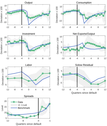
Figure1displays a typical default episode by plotting key series 12 quarters before and after
a default in our sample of emerging economies. As described more fully in AppendixA.1, the
data are for nine countries (except for spreads, which are available only for Argentina and
Ecuador) and quarterly (except for labor and the Solow residual, which are only available
annually).6 The green dotted lines represent deviations from an HP-filtered trend (the
stan-dard smoothing parameter value of 1600 is used) except for the spreads, which are reported in levels. The shaded areas correspond to plus- and minus-one-standard deviations around
the mean, and the blue solid lines are the predictions from our benchmark model.
The default episodes have a clear boom-bust-recovery pattern. The boom is characterized
by above-trend growth in output, consumption, investment, and productivity that peaks
around one year before default (marked with the vertical black line) with falling spreads. The
boom gives way to a decline in output, consumption, investment, labor, and productivity,
as well as an increase in spreads. While the decline is gradual at first, it becomes severe
in the period immediately before default and stays that way for around a year. While the
patterns are similar for output, consumption, and investment, the 5% decline in output and consumption at default is dwarfed by the 20% drop in investment. In fact, at the country
level, the decline in investment can be as large as 44% like it was in Argentina’s 2001 default.
While the worst of the crisis is over within a year, a full recovery takes around two years,
and even then productivity remains below trend. With few exceptions, the model correctly
and the excess consumption volatility (0.95 vs. 1.23). Roldan-Pena (2012) fails along these dimensions as well while also not reporting the mean spread and having a default rate of only 0.07%.
Output
-12 -8 -4 0 4 8 12
-10 -5 0 5 10
Deviation x 100
Consumption
-12 -8 -4 0 4 8 12
-10 0 10
Deviation x 100
Investment
-12 -8 -4 0 4 8 12
-20 0 20
Deviation x 100
Net Exports/Output
-12 -8 -4 0 4 8 12
-5 0 5 10
Deviation x 100
Labor
-12 -8 -4 0 4 8 12
-5 0 5
Deviation x 100
Solow Residual
-12 -8 -4 0 4 8 12
Quarters since default
-5 0 5
Deviation x 100
Spreads
-12 -8 -4 -1
Quarters since default
5 10 15 20
Level
Data +/- 1 s.d. Benchmark
captures the boom, bust, and recovery, and it does so with output, consumption, investment,
and spreads all determined endogenously.
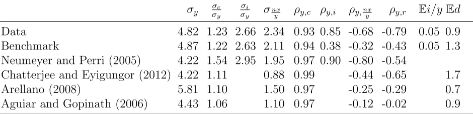
The model also correctly predicts the behavior of these variables in normal times. This
can be seen in Table 1, which compares Argentinean data and the model, as well as key
papers in the literature (which we will revisit in much more detail in Section 6). The data
exhibit typical elements of fluctuations in emerging economies such as highly volatile output,
excessive volatility of consumption, countercyclical net exports, and countercyclical spreads,
and—like many of the existing papers in the literature—our model captures these features.7
For instance, we match business cycle properties likeNeumeyer and Perri(2005) and default
rates like Arellano (2008). The difference is that our model simultaneously captures these features and it does so with output, consumption, investment, net exports, spreads, and
default all determined endogenously.
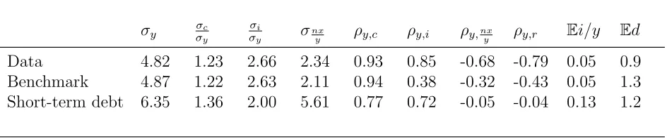
σy σσyc σσyi σnxy ρy,c ρy,i ρy,nxy ρy,r Ei/y Ed
Data 4.82 1.23 2.66 2.34 0.93 0.85 -0.68 -0.79 0.05 0.9 Benchmark 4.87 1.22 2.63 2.11 0.94 0.38 -0.32 -0.43 0.05 1.3 Neumeyer and Perri (2005) 4.22 1.54 2.95 1.95 0.97 0.90 -0.80 -0.54
Chatterjee and Eyigungor (2012) 4.22 1.11 0.88 0.99 -0.44 -0.65 1.7 Arellano (2008) 5.81 1.10 1.50 0.97 -0.25 -0.29 0.7 Aguiar and Gopinath (2006) 4.43 1.06 1.10 0.97 -0.12 -0.02 0.9
Note: σ and ρ denote volatility and correlation, respectively. Output, consumption, invest-ment, net exports, spreads, and default are denoted by y, c, i, nx, r, and d, respectively. Series are logged and HP-filtered except for r, nx/y, i/y, and d. See Table 5 for details on the referenced papers.
Table 1: Moments in Data and Model
3
Model
In the tradition of sovereign default models begun byEaton and Gersovitz(1981), we assume
a sovereign borrows in international markets to maximize the welfare of citizens living at home. Domestic residents have consumptionc, supply labor l, and rank consumption/labor
bundles according to
E0
∞
X
t=0
βtu(ct, lt).
In the computation, we use Greenwood, Hercowitz, and Huffman (1988) preferences of the
formu(c, l) = (c−ηlωω)1−σ/(1−σ). The sovereign has access to a technology that uses capital
kand laborlto produce outputyusing the Cobb-Douglas functiony=Akαl1−α. We assume
that productivity follows logA0 = (1−ρA) logµA+ρAlogA+ε0A where εA ∼ N(0, σA2). In
addition to endogenous output, the sovereign has an iid endowmentmdrawn from a bounded
normal with standard deviationσm and support [m, m]. AsChatterjee and Eyigungor(2012)
show, incorporating even a small iid shock greatly facilitates computation, which is its role
here. Our computational algorithm is given in Appendix A.6.
The sovereign government has access to long-term debt contracts in which outstanding
debt matures with probability λ.8 If debt does not mature, it delivers a coupon paymentz. As shown by Chatterjee and Eyigungor (2012) (and Hatchondo and Martinez, 2009, with
z = 0), this memoryless debt structure can capture average debt maturities in the data
without making computation overly onerous. Following the convention in the literature,
we treat debt as negative bond holdings. Current bond holdings are denoted b, which we
restrict to be negative.9 The contract structure implies that new debt issuance is given by
−b0+ (1−λ)b (if negative, then existing debt has been repurchased). Bonds are discounted by the price q.
A default has four consequences for the sovereign. First, its debt goes away. Second, it is
excluded from credit markets (i.e., goes to autarky). Third, it is readmitted to credit markets with probabilityφ. Last, for the duration of autarky, a fractionκ of output is lost. This last
assumption captures in part what is endogenized in Mendoza and Yue (2012), namely, that
default impairs a country’s ability to produce by limiting its access to imports. Since capital
refers to assets physically located within the borders of an economy, we further assume that
capital cannot be expropriated in default and cannot be pledged as collateral.
When the sovereign has access to financial markets, it decides whether to repay debt and,
if so, how much new debt to issue subject to households’ preferences, technology, and the
economy’s resource constraint.10 In particular, the sovereign solves
V (b, k, m, A) = max
d∈{0,1}(1−d)V
nd(b, k, m, A) +dVd(k, A) (1)
8Arellano and Ramanarayanan (2012) and Sanchez, Sapriza, and Yurdagul (2014) endogenize debt ma-turity, but doing so here would be computationally infeasible.
9In the computation, bonds, capital, and productivity lie in finite sets.Chatterjee and Eyigungor(2012) prove existence of equilibrium with exogenous output using finite sets for bonds and output. The main theoretical advantage of using finite sets is that the price scheduleqis a vector rather than a function. The restriction of bonds being negative is imposed to reduce the computational burden (but is rarely if ever binding in our calibration).
wheredis the default choice,Vnd is the value of repaying debt (i.e., not defaulting) andVdis
the value of entering or being in autarky. Consistent with our assumption of no expropriation,
capital remains a state variable after default.
The value of repaying debt is
Vnd(b, k, m, A) = max
c,l,k0≥0,b0≤0u(c, l) +βEm0,A0|AV (b
0
, k0, m0, A0)
s.t. c+i+q(b0, k0, A)(b0 −(1−λ)b) =Akαl1−α+m−Θ
2 (k
0−
k)2+ (λ+ (1−λ)z)b
k0 =i+ (1−δ)k,
(2)
wherei is investment and Θ controls the cost of adjusting capital. The term (λ+ (1−λ)z)b
captures payments from the fractionλof debt that matures and the coupon from the fraction
(1−λ) that remains outstanding. The termq(b0, k0, A)(b0−(1−λ)b) reflects any income from
new bond issuance or repurchases.
As already argued, a key contribution of this paper is the inclusion of capital accumulation
in a way that captures the dynamics of investment found in the data. To this end, we found
it necessary to include a variable adjustment cost paid any time the capital stock deviates
from its previous value. This is because—without adjustment costs—negative productivity
shocks result in two effects that make investment fluctuate drastically. First, a negative shock makes the sovereign want to smooth consumption by borrowing against future higher
productivity. Second, such a shock also increases the sovereign’s default probability and so
causes interest rates on debt to rise. Without adjustment costs, the cheapest way for the
sovereign to “borrow” is by sharply reducing investment rather than borrowing on the world
market. Consequently, investment ends up being too volatile relative to the series in the data.
Adjustment costs make borrowing using capital more costly and so tame the fluctuations in
investment.11
The value of defaulting or being in autarky is
Vd(k, A) = max
c,l,k0≥0u(c, l) +βEm0,A0|A
(1−φ)Vd(k0, A0) +φV(0, k0, m0, A0)
s.t.c+i= (1−κ(A))Akαl1−α−Θ
2(k
0 − k)2
k0 =i+ (1−δ)k.
(3)
Note that when the economy regains access to credit markets (which happens with
proba-bility φ), the sovereign has no debt. In the quantitative work, we assume that κ(A) is given
by
κ(A) = min (max (κ0+κ1A,0),1),
which captures the asymmetric losses used in Arellano (2008), Chatterjee and Eyigungor
(2012), and others. The assumption that the cost depends on the state of technology (rather
than output) allows for a straightforward computation of the labor choice.
For a bond levelband capital stockk, it is optimal to default for total factor productivity
(TFP) values and iid shock values in
D(b, k) = A, m :Vnd(b, k, m, A)< Vd(k, A) . (4)
In the absence of capital, it is well understood that the default set shrinks withb, i.e., lower
debt increases the likelihood of repayment (Arellano,2008;Chatterjee and Eyigungor,2012;
Mendoza and Yue, 2012). Because Vnd is increasing in b, the same result obtains here: D is
monotonically decreasing in b.12
Unfortunately, characterizing how the default set varies in capital is much more difficult. The first and obvious obstacle is that the value functionsVnd and Vdmay not be monotonic
in capital due to capital adjustment costs. Second, even with monotonicity for each value
function, a change in the capital stock can have uneven effects on the two value functions and
cause the spreadVnd−Vdto vary in non-trivial ways. In fact, we will show quantitatively that
this spread does vary unevenly (see Figure 6). Hence, the inequality in (4) might fluctuate,
which prevents a simple characterization of the default set with respect to capital.
A major difference in our model relative to previous ones is that the default decision,
and consequently the price of debt, depends on capital and productivity rather than an
exogenous output level. In particular, the equilibrium debt prices implied by risk-neutral foreign lenders making zero profits loan-by-loan are given by
q(b0, k0, A) =Em0,A0|A(1−d(b0, k0, m0, A0))
λ+ (1−λ) [z+q(b00, k00, A0)]
1 +r∗ (5)
whereb00=b0(b0, k0, m0, A0),k00 =k0(b0, k0, m0, A0), andr∗ is the risk-free international rate on
a one-period bond. If the sovereign repays next period, creditors receive back theλfraction of
the debt that comes due plus the couponzand market valueq(b00, k00, A0) for the 1−λfraction
of debt that does not mature. If the sovereign defaults, they receive nothing. Since the model
12For any choice of l, k0, b0, an increase inb produces increased consumption in the Vnd problem. This
weakly expands the set of feasible choices and makes already feasible choices deliver more utility, implying
is already challenging to solve, we follow Arellano(2008);Chatterjee and Eyigungor(2012);
and Mendoza and Yue(2012) and abstract from the important issue of debt renegotiation.
Yue (2010) and Bai and Zhang (2012a) provide an excellent discussion of default and debt
renegotiation.
Before turning to the quantitative aspects of our model, it is worth discussing our
assump-tion that the sovereign chooses all allocaassump-tions. In AppendixA.2, we show that a combination
of state-contingent capital taxes, labor taxes, and lump-sum taxes are sufficient to support
the sovereign’s chosen allocations in a decentralized economy where households choose labor
and capital investment. At the optimal allocation, the labor tax is always zero while the
optimal capital tax τk is given by13
τk= ∂q(b
0, k0, A)
∂k0 (b
0−
(1−λ)b)
in repayment and zero in default. As we will show, quantitativelyqis almost always increasing
in capital. Consequently, in the model it is optimal to subsidize investment when issuing
new debt (b0 <(1−λ)b), neither tax nor subsidize when just paying off debt that matures (b0 = (1−λ)b), and tax investment when repaying debt (b0 >(1−λ)b).
4
Calibration
Our calibration approach follows the default literature closely. Taking a period to be a quarter, the benchmark adopts the long-term debt structure in Chatterjee and Eyigungor
(2012) where the coupon payment is 3% (z =.03) and debt matures with a 5% probability
(λ=.05). These nearly match the Argentinean data’s 20 quarter median maturity of average
bonds and 11% value-weighted average coupon rate (Chatterjee and Eyigungor, 2012, p.
2685).14Our short-term debt calibration hasλ = 1 (with the coupon irrelevant). The support
of the continuous shock m is the same as in Chatterjee and Eyigungor (2012). Following
Aguiar and Gopinath (2006),φ is set to .1 which generates an average stay in autarky of 2.5
years.
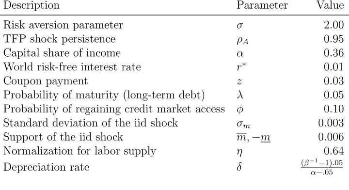
The rest of the independently determined parameters are reported in Table 2, and some of these are worth mentioning. Given the lack of reliable labor data, we followNeumeyer and
Perri (2005) and set the persistence of TFP to be .95 (which is in line with the values used
13The capital tax applies to the stock of next period’s capital, i.e., capital tax revenue isτkk0.
Description Parameter Value
Risk aversion parameter σ 2.00 TFP shock persistence ρA 0.95
Capital share of income α 0.36 World risk-free interest rate r∗ 0.01
Coupon payment z 0.03
Probability of maturity (long-term debt) λ 0.05 Probability of regaining credit market access φ 0.10 Standard deviation of the iid shock σm 0.003
Support of the iid shock m,−m 0.006 Normalization for labor supply η 0.64 Depreciation rate δ (β−1α−−.1)05.05
Table 2: Parameter Values Calibrated Independently
in the emerging-economy business-cycle literature such as Fernandez-Villaverde,
Guerron-Quintana, Rubio-Ramirez, and Uribe, 2011 and Mendoza and Yue, 2012). Conditional on
the other parameters, we choose mean productivityµA and the labor disutility parameter η
so that, in the steady state without foreign lending, output and labor both equal 1. Likewise,
the depreciation rateδ is set to deliver an investment-GDP ratio of 0.05 (which is the value
for Argentina) in the steady state without foreign lending. The utility function curvature σ
is set to a standard value of 2.
The second group of parameters is chosen to match empirical moments. There are six parameters in this group: the discount factor β, the default cost parameters κ0 and κ1,
the cost of adjusting capital Θ, the volatility of productivity σA, and the labor elasticity
parameter ω. These were chosen to match six empirical moments: the debt-output ratio
−Eb/y, the average spread Er, the spread volatility σr, the volatility of investment σi, the
volatility of output σy, and the ratio of the volatilities of consumption and output σc/σy.
As in Chatterjee and Eyigungor (2012), we measure the spread as the difference between
an annualized “internal rate of return”—an ˜r satisfying q = (λ+ (1−λ)z)/(λ+ ˜r)—and
the annualized risk-free rate. The resulting parameter values, target moments, and model
Jointly Calibrated Parameters
Description Value Short Long
Discount factor β 0.449 0.946
Fixed default cost κ0 -0.07 -0.26
Proportional default cost κ1 0.10 0.66
Adjustment cost Θ 7.91 21.16
TFP innovation size σA 0.016 0.017
Labor supply elasticity 1/(ω−1) 0.85 1.57
Targeted Statistics
Target Value Short Long
Debt-output ratio∗ (−Eb/y) 0.70 0.66 0.70 Average spread∗ (Er) 8.15 5.23 8.20 Standard deviation of spread∗ (σr) 4.43 4.06 4.41
Standard deviation of investment∗∗ (σi) 12.8 12.7 12.8
Standard deviation of output∗∗ (σy) 4.82 6.35 4.87
Excess consumption volatility∗∗ (σc/σy) 1.23 1.36 1.22
∗Sample excludes 20 periods after default (as in Chatterjee and Eyigungor,2012). ∗∗Full sample, series is logged and HP-filtered before statistics are calculated.
5
Results
We begin this section by analyzing the model’s behavior in default episodes. As will be
seen, the benchmark model outperforms the short-term debt model substantially. We then
examine why the short-term debt model fails before turning attention to other properties of
the benchmark. The section concludes with an in-depth examination of the role of capital in
the decision to default.
5.1
Default Episodes
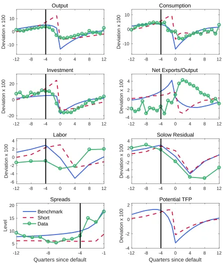
Figure2displays the dynamics of a typical default episode in the data, our benchmark
cali-bration, and the short-term debt calibration. Relative to short-term debt (red dashed lines), the benchmark model (blue solid lines) does a superior job of matching the data’s slow
tran-sition to default. Also consistent with the data (green dotted lines), the benchmark predicts
that the economy peaks a few quarters before repayments are stopped (the black vertical
line marks one year prior to default). In the benchmark, it takes investment, consumption,
and output roughly 10 quarters to return to trend post-default, which is very similar to the
data. In contrast, short-term debt, despite a shallower decline at the time of default, takes
longer to recover. While both the benchmark and short-term debt version miss on the labor
series, the benchmark’s accurately captures the run up in spreads preceding default that
the short-term debt calibration almost completely misses. Overall, default episodes in the benchmark closely capture default episodes in the data, and the same cannot be said for the
short-term debt calibration.
The proximal reason for why the short- and long-term debt calibrations differ is tied to
the sequence of productivity shocks leading to default (the bottom, right panel in Figure
2). (In the figure, the “Potential TFP” series gives A—which is TFP when the sovereign
repays their debt—while the “Solow Residual” series gives Ain repayment and (1−κ(A))A
in default—which is TFP inclusive of default costs.)15 For the benchmark, productivity (A)
peaks about a year before default and is followed by a gradual decline. In contrast, the
short-term specification has productivity steadily increasing until default. For both calibrations, output, consumption, and investment comove with productivity. For the benchmark, this
re-sults in gradual increases and decreases leading up to default. For the short-term calibration,
it results in all these measures rising steadily until default.
Both calibrations wrongly predict a trade surplus prior to default and a trade deficit
after default. To understand the latter failure, note that net exports in the economy can be
-12 -8 -4 0 4 8 12 -10
0 10
Deviation x 100
Output
-12 -8 -4 0 4 8 12
-10 0 10
Deviation x 100
Consumption
-12 -8 -4 0 4 8 12
-20 0 20
Deviation x 100
Investment
-12 -8 -4 0 4 8 12
-4 -2 0 2 4
Deviation x 100
Net Exports/Output
-12 -8 -4 0 4 8 12
-6 -4 -2 0 2 4
Deviation x 100
Labor
-12 -8 -4 0 4 8 12
-6 -4 -2 0 2 4
Deviation x 100
Solow Residual
-12 -8 -4 -1
Quarters since default
5 10 15 20 Level Spreads Benchmark Short Data
-12 -8 -4 0 4 8 12
Quarters since default
-4 -2 0 2
Deviation x 100
Potential TFP
written asN X =q(b0−(1−λ)b)−(λ+(1−λ)z)b. When a sovereign defaults,bis set to 0 and,
for as long as the sovereign remains in autarky, both b0 and N X are 0. When the economy
is readmitted to financial markets, their new bond position is restricted to be negative and
so N X must be less than 0. Hence, the economy must run a trade deficit after default.16
To see why the benchmark runs a trade surplus prior to default, consider that the change
in net exports is given by ∆N X = −x∆q−q−1∆x+ (λ+ (1−λ)z)∆(−b) where x is new
debt issuance, −b0+ (1−λ)b.17 Until six quarters before default, productivity and capital
are both increasing. As we will show, both of these cause ∆q >0 else equal. The sovereign,
who is impatient relative to lenders, takes advantage of this to borrow on world markets. In
fact, from 12 quarters to 6 quarters before default, the level of debt increases 6% on average, which makes x, ∆x, and ∆(−b) all positive. The change in net exports is ambiguous in
this case. However, when productivity starts declining around 6 quarters before default, this
causes a decline in q. In response to ∆q < 0, the sovereign typically just rolls over its debt:
From 6 quarters to the period of default, debt increases by only 0.7%. Hence, typically one
has ∆q < 0, x > 0, and ∆x and ∆(−b) both nearly 0. This unambiguously drives up net
exports. While the model’s prediction of a trade surplus pre-default differs from the average
in the data, it is in fact consistent with the default episodes of Indonesia (1998.Q3), Peru
(1983.Q2), and South Africa (1998.Q1).
5.2
Short-Term Debt
As can be seen in column “Short” of Table 3, the short-term debt calibration comes fairly close to reproducing the targeted moments. This matching, however, comes at the price of
a very low discount factor, β = 0.45, and even then fails to deliver large enough spreads
and small enough consumption volatility. The high impatience of the planner is a common
feature of default models, but the value here is well below the values in, for example,Aguiar
and Gopinath (2006) and Mendoza and Yue (2012).
To see why the short-term debt model fails to match the targeted moments for
con-ventional parameters, consider the results of a prior predictive exercise in which the model
is solved hundreds of times for randomly chosen parameter values. As we explain more
thoroughly in Appendix A.3, we draw each of the parameters β, κ0, κ1,Θ, σA, and ω from
16This is a feature common to most sovereign default models. An exception is that ofMendoza and Yue (2012), where the trade balance improves following default. In their model, upon default the sovereign has access, albeit limited, to intermediate imported goods. This means that if imports of these goods drop sufficiently (as they do in their paper), the economy can experience a trade surplus following default.
17To see this, write net exports in a given period as N X = −qx+ (λ+ (1−λ)z)(−b). Then ∆N X =
distributions whose bounds cover standard values used in the literature.18 For example, β is
drawn from a uniform distribution with support [0.9,0.99].
0 5 10 15 20 25 30 35 40
0 0.5 1 1.5 2 2.5 3
Debt-output ratio
Short-term debt Long-term debt Target
0 5 10 15 20 25 30 35 40
Mean spread (%) 0
10 20 30 40 50
Spread standard deviation (%)
Figure 3: Prior Predictive Draws for Short- and Long-term Debt
Figure3displays the implied spread mean, spread standard deviation, and average
debt-output ratio for each of these draws. Evidently, the model with short-term debt cannot
simultaneously match the debt and interest rate moments. E.g., the model generates high
average spreads at the expense of an overly small debt-to-output ratio and overly large
spread volatility. Alternatively, data-consistent levels of debt and volatilities of spreads lead inexorably to low average spreads. In contrast, long-term debt allows the model to easily
match the targeted moments along these dimensions.
The short-term debt model’s struggle to match the targeted moments for conventional
parameters pushes it away from non-targeted moments. Table 4 contains select moments
from the Argentinean data and short-term debt model (a σ denotes a standard deviation,
a ρ denotes a correlation, and an E denotes an average).19 For instance, the model fails to
produce a countercyclical trade-balance (ρy,nxy is −.05 in the model but −.68 in the data)
18For parameters like κ
0 and κ1 for which the literature offers little guidance, we tried to draw from a wide range of values.
and countercyclical spreads (ρy,r is −.04 in the model but −.79 in the data). Likewise,
consumption is procyclical, but not as procyclical as in the data (ρy,cis.77 in the model and
.93 in the data). These failures can be traced back to the low discount factor. Because the
discount factor is so low, the limiting factor on sovereign debt issuance is not the supply of
debt but the demand for it, q(·,·, A). Hence, when productivity increases, so does q, and so
does sovereign borrowing. This ties consumption, interest rates, and net exports more closely
to productivity than output, the latter depending on slow-moving capital.
The short-term debt model nearly matches the data’s investment volatility and
procycli-cality but deviates substantially from the investment-output ratio. Recall that depreciation
is set to give a 5% investment-output ratio in the steady state without foreign lending. In fact, the short-term debt model is very far away from this steady state: Average output in
the ergodic distribution of the model is 2.8 times larger than in the steady state. The reason
clearly is not due to the patience of the sovereign. Rather, it is because debt is cheaper at
higher levels of capital (as will be discussed). Consequently, the incentive to save using k0
comes from a desire to increase current consumption by borrowing from foreign markets.20
σy σσc
y
σi
σy σ
nx
y ρy,c ρy,i ρy, nx
y ρy,r Ei/y Ed
Data 4.82 1.23 2.66 2.34 0.93 0.85 -0.68 -0.79 0.05 0.9 Benchmark 4.87 1.22 2.63 2.11 0.94 0.38 -0.32 -0.43 0.05 1.3 Short-term debt 6.35 1.36 2.00 5.61 0.77 0.72 -0.05 -0.04 0.13 1.2
Note: Data for σ and ρ are logged and HP-filtered except for r and nx/y. The data measure for Ed is the 3.8% annual rate reported in Tomz and Wright (2013). Ar-gentina’s sample is 1993.Q1 - 2011.Q3.
Table 4: Moments in Data and Model
All told, the model with short-term debt can capture some of the features of the data
if one assumes that emerging economies are extremely impatient. However, this tremendous
impatience results in other distortions, including the failure to match output, consumption,
and investment dynamics around default. We now show that long-term debt goes a long
way toward bringing the model closer to the data while using more conventional parameter
values.
5.3
Long-Term Debt
The column “Long” in Table3shows that our baseline model matches the targeted moments
and that it does so with a more realistic discount factor and a labor elasticity closer to the
values commonly used in the literature (specifically, those in Mendoza and Yue, 2012 and
Neumeyer and Perri, 2005). In fact, the prior predictive exercise in Figure 3 reveals that
the long-term debt model could match the targeted interest rate with a debt-output ratio nearly three times as large as the data’s while still using conventional parameter values. The
model also does a superior job matching Argentina’s business cycles, as can be seen from
the “Benchmark” panel in Table4. For example, it captures simultaneously the volatility of
output and of net exports. These findings agree with and extend those in Chatterjee and
Eyigungor (2012), namely, that long-term debt is essential for matching debt, interest rate,
and net export statistics. Although the model correctly predicts the countercyclicality of the
trade account, it falls short of delivering its magnitude (this is also the case in Arellano,
2008; Chatterjee and Eyigungor, 2012; and Mendoza and Yue, 2012). The quarterly default
rate is 1.3%, which is somewhat larger than the data’s 0.9%.
With regards to the investment statistics, the calibration delivers procyclical investment
with a correlation of .38, qualitatively correct but falling short of the .85 in the data.21 While
the model misses the magnitude of this correlation, it produces the correct comovement in
default episodes (as can be seen in Figure 2). The investment-output ratio is .05, the same
as in the data. This moment is important because, in the spirit of incomplete market models
(e.g., Aiyagari, 1994), the sovereign can use capital to hedge against bad outcomes. That is,
having more capital ameliorates the cost of defaulting because capital can be transformed
into consumption goods.
The benchmark model also captures the data’s significant negative correlation between output and spreads. Neumeyer and Perri (2005) argue that this negative correlation is a
crucial feature of emerging small open economies that the standard small open economy
RBC model without working capital fails to generate. In our model, two forces shape the
correlation between output and spreads. One force is the endogenous pricing of default risk:
As productivity declines, spreads increase and output contracts, which tends to result in a
negative correlation. The other force is the RBC implication of a negative productivity shock
reducing expected returns to capital. The lower return to capital induces the sovereign to
rebalance its portfolio until the return on capital is similar to the return on bonds, which
potentially decreases spreads.22 This force tends to result in a positive correlation. Our
cali-bration gives that the first force dominates, which delivers the correct sign for the correlation.
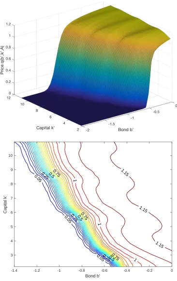
We now turn to the implications of capital accumulation on the price of debt. The upper
panel in Figure 4 shows the bond price schedule along the capital and bond dimensions
conditional on a typical level of productivity (in our figures, debt is expressed as a fraction
of output in steady state, which is normalized to 1). For a given capital value, we obtain
the standard result that lower levels of debt are associated with higher bond prices. More
importantly, the figure reveals one key result of this paper: Additional capital helps sustain higher levels of debt. This beneficial impact of capital on debt is also seen in the “iso-price”
graph in the lower panel of Figure 4. Specifically, this graph plots (b0, k0) pairs delivering a
particular price q (i.e., {(b0, k0)|q(b0, k0, A) =q} for differing values of q). For q close to the
risk-free price, capital typically helps sustain more debt. For small and moderate values of
q, this is always the case.
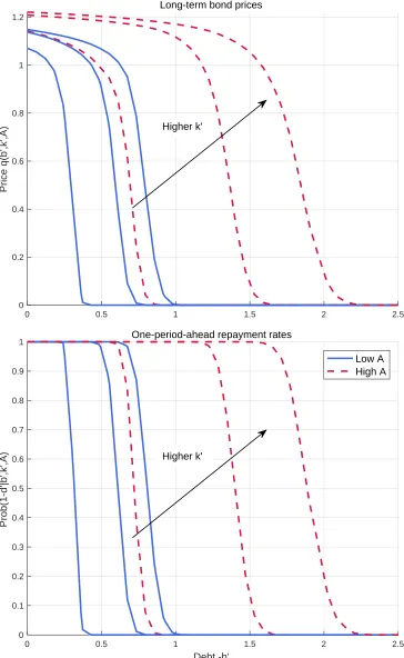
To shed more light on how capital affects debt prices, the upper panel of Figure 5
dis-plays the price schedule for three different levels of capital (the smallest, median, and largest
values on our grid) conditional on two levels of productivity (corresponding to ±2 standard
deviations from the mean). The lower panel does similarly, but for the one-period-ahead re-payment rateEm0,A0|A(1−d(b0, k0, m0, A0)). For clarity, the horizontal axis corresponds to debt
(−b0) and the arrow indicates the direction in which capital increases. At the lowest capital
and productivity levels, debt (as a fraction of steady-state output) starts being demanded
(i.e., q > 0) at around −b0 = 0.4. As capital moves to the largest value, debt starts being
valued at around b =−1, a value roughly 2.5 times larger. Similar dynamics occur at high
productivity levels. One can see that more capital raises the price of debt for virtually any
debt level.
Figure 5also reveals that capital reduces the odds of default not just in the next period
but well into the future. At low levels of capital, each additional unit increases the one-period-ahead repayment rates (as can be seen in the bottom panel). This results in lenders
being willing to lend at low spreads, which increases debt prices. But more capital also
increases bond prices even when the probability of repayment next period is 1. E.g., for any
0.05 0.05
0.05
0.25 0.25
0.25
0.5 0.5
0.5
0.75 0.75
0.75
1 1
1
1.15 1.15 1.15
-1.4 -1.2 -1 -0.8 -0.6 -0.4 -0.2 0
Bond b' 3
4 5 6 7 8 9 10
Capital k'
0 0.5 1 1.5 2 2.5 0
0.2 0.4 0.6 0.8 1 1.2
Price q(b',k',A)
Long-term bond prices
Higher k'
0 0.5 1 1.5 2 2.5
Debt -b' 0
0.1 0.2 0.3 0.4 0.5 0.6 0.7 0.8 0.9 1
Prob(1-d'|b',k',A)
One-period-ahead repayment rates
Low A High A
Higher k'
debt amount less than .2, the sovereign repays next period with probability 1 for each level
of capital. But, additional capital increases the debt price anyway because debt is long-term
and additional capital tomorrow results in additional ability to pay well into the future.
These results are consistent with the empirical observation that developed countries, i.e.,
countries with large capital stocks, seem less likely to default.
Relatedly, we find that—for regions of debt having positive prices for all capital levels—
the price schedule typically displays decreasing returns to capital. For instance, when debt
is 0.5 and productivity is high, the price of debt jumps from 1 to around 1.18 when capital
increases from the lowest level in the grid to the median (an 18% increase). In contrast,
when the stock of capital moves from the median to the highest capital stock, the price moves from 1.18 to 1.20 (only a 2% increase). Since the capital grid is linearly spaced, this
implies decreasing returns.
This finding is explained by the effects of increased repayment rates at different horizons.
When capital causes the one-period-ahead repayment rate to increase, this has a first-order
effect on the price schedule in (5) by increasing principal and coupon repayments as well
as the market value of remaining debt. In contrast, the effect of a capital increase when
repayment rates are 1 (or very high) is second-order: It only increases the current price
by increasing the future price of debt that does not come due. This naturally generates
diminishing returns to capital when debt is long-term.
5.4
Dissecting the Role of Capital
As discussed in the introduction, capital causes a tension. More capital gives the planner
a savings tool to weather bad times and either avoid or postpone default. However, it also
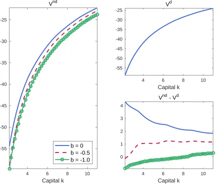
increases the benefit of defaulting since the value of autarky rises with capital. To illustrate
these forces, we plot in Figure 6 the value functions of repayment (Vnd, left panel), default
(Vd, right upper panel), and their difference (Vnd−Vd, right bottom panel) as a function
of capital for three levels of debt with productivity at its median level and m = 0.
The interplay between debt and capital is nontrivial. For instance, when the country is
deeply indebted (which corresponds to the green circled line), additional capital improves
the sovereign’s ability to repay faster than it improves the value of autarky. This is reflected in the spread Vnd−Vd being increasing in k. That is, the smoothing channel of increased
capitalVnd
k dominates the autarky channel Vkd at large levels of debt. In contrast, when the
sovereign has little debt (like in the solid blue line), the spread is decreasing in capital, which
implies that the autarky channel dominates the smoothing channel.
4 6 8 10
Capital k
-55 -50 -45 -40 -35 -30 -25
Vnd
b = 0 b = -0.5 b = -1.0
4 6 8 10
Capital k
-55 -50 -45 -40 -35 -30 -25
Vd
4 6 8 10
Capital k
0 1 2 3 4
Vnd - Vd
andVd would be if leisure were not valued, there were no adjustment costs, and the problem
were smooth:
Vknd =u0(cnd)(1 +Aαkα−1−δ) and Vkd=u0(cd)(1 + (1−κ)Aαkα−1−δ). (6)
For sufficiently large debt levels, repaying or rolling over debt is costly, causing cnd cd.
Hence, Vknd−Vkd>0 and the spread is increasing in capital. In contrast, for small amounts of debt, repaying debt is trivial but default costs are not. This causes cnd to typically be
greater thancd, and so the spread is decreasing in capital (Vnd
k −Vkd <0).
Another feature evident in Figure 6 is that the concavity or convexity of the spread also
hinges on the level of debt: For large levels of debt, the spread is concave; for low levels, the
spread is convex. To see cleanly why this is, consider differentiating the envelope condition
in (6) again while eliminating the impact of capital on its marginal product by settingα = 1.
Then,
Vkknd =cndk u00(cnd)(1 +A−δ) and Vkkd =cdku00(cnd)(1 + (1−κ)A−δ). (7)
For constant relative risk aversion of σ, the definition of relative risk aversion givesu00(c) =
−σu0(c)/c. Using this to replace u00 in (7) and simplifying gives
Vkknd =−σndVknd and Vkkd =−σdVkd,
wherend and d, defined asdlogcnd/dk anddlogcd/dk, are elasticities of consumption with
respect to capital. Putting these together, one has
Vkknd−Vkkd =−σd
nd
d V
nd k −Vkd
.
For large levels of debt, repaying or rolling over debt is costly since debt pricesqare low. Given
extra capital, the sovereign can choose a combination of (b0, k0) that results in an improved
priceq, which improves consumption beyond just the direct effect of additional capital. This
makesndlarge relative todfor large levels of debt. As a consequence, the term in parentheses
is positive and the spread is concave. For smaller levels of debt, nd is smaller because now
the sovereign does not need to service debt at high-interest. In contrast, a sovereign in default would generally like to borrow against the future when the default penaltyκ is gone
and hence output is higher. Given an additional unit of capital, the sovereign then finds it
optimal to consume most of it. Hence, d> nd at low levels of debt, which makes the term
in parentheses negative and results in a convex spread.
a sovereign that chooses to repay benefits greatly from extra capital because of the direct
effect of additional output and the indirect effect of lower debt service costs. Relative to a
sovereign in default who only has the direct effect, additional capital improves the sovereign’s
situation quickly. Once the indirect effect is gone (in the high debt case with lots of capital)
or if it is not present (as in the low debt case), it is the sovereign in default who benefits the
most: Consumption smoothing dictates that they consume more in the present, and extra
capital enables them to do so.
Since the spreadVnd−Vdis decreasing in capital for low levels of debt, a one-period debt
framework would suggest that the price of small levels of debt decrease as capital increases.
Why, then, does the opposite result obtain? It is because debt is long term. High capital today results in higher average levels of capital several periods in the future when, typically,
the country will be more indebted. It is there where additional capital, resulting in reduced
future default probabilities, comes to bear and results in a higher current price.
-10 -5 0 5 10
Time since default -15
-10 -5 0 5 10
HP-filtered log investment
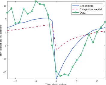
Benchmark Exogenous capital Data
Figure 7: Investment Dynamics around Default
An alternative way to examine the role of capital is by studying an economy in which
investment follows a policy rule outside of the planner’s control. Under this assumption,
investment loses its role in the smoothing channel and retains only its role in the autarky
we obtain an exogenous investment policy by solving an RBC version of our model in which
the sovereign chooses anyk0 but cannot borrow, i.e.,b0 = 0. For technical reasons, we assume
that this k0 applies to the entire interval [m, m] and that the sovereign chooses it assuming
m = m.23 In the second step, we use this exogenous investment policy function, together
with the autarky value function and autarky capital policy from the benchmark, but allow
the sovereign to optimally choose b0 and for prices to respond. Once again, we assume that
the b0 applies to the entire interval and that it is chosen assuming m=m.24
Figure 7 displays the dynamics of investment during default for both the benchmark
model (solid blue line) and when capital is exogenously determined (red dashed line). In
the benchmark, the planner reduces investment in the periods prior to default to prop up consumption at a time when the economy is being buffeted by negative productivity shocks
(the productivity decline can be seen in Figure 2). In contrast, when investment is not a
choice variable, the central planner defaults when the stock of capital is at its highest level.
The reason is two-fold. First, the planner internalizes the benefit that capital has on the
value of autarky. Second, the planner wants to liquidate some capital in order to smooth
consumption and avoid default, but he cannot as investment is outside of his control: The
smoothing channel is absent.
The crucial smoothing role of investment prior to default is further exposed in Table 5.
There we compare the dynamic properties of the model with exogenous capital accumulation (the row labeled “Exogenous Capital”) and those of the benchmark. The exogenous capital
case induces excess consumption volatility of 1.36 compared to the benchmark’s 1.22: The
sovereign cannot use investment to avoid default or mitigate the effects of fluctuations in
foreign lending.
6
Alternative Models
In this section, we compare our model and small variations on it against a few existing models that have explained important features of small open economies. We group the models into
three categories: RBC models with exogenous interest rates (Neumeyer and Perri, 2005),
models with sudden stops (Mendoza, 2010), and sovereign default models with exogenous
output (Aguiar and Gopinath, 2006;Arellano, 2008; Chatterjee and Eyigungor, 2012).
6.1
RBC with Exogenous Interest Rates
Neumeyer and Perri (2005) construct a small open economy model with exogenous interest
rates that successfully captures many important features of business cycles in emerging
economies. We allow for a small open economy RBC version with exogenous interest rates
in our model through two modifications. First, we replace the budget constraint with
c+q(b0−(1−λ)b) +i=Akαl1−α−Θ
2 (k
0−
k)2− Φ
2(b
0−¯
b)2+ (λ+ (1−λ)z)b.
Here, Φ is a small constant allowing for the model to be solved by linearization, and ¯b is a
target stock of debt. Second, we assume that q follows the stochastic process given by
q= (λ+ (1−λ)z)/(λ+r∗+s)
s0 = (1−ρs)¯s+ρss+σs0s.
The persistence ρs of the spread shocks is taken from Neumeyer and Perri (2005). The
target debt level ¯b and the average spread ¯s are set to match the debt-output ratio and the
annualized average spread in the data (0.70 and 8.15, respectively). As in the benchmark model, we normalize steady state output to 1.
The calibration strategy for the remaining parameters is nearly as before. The TFP shock
sizeσAis used to match the volatility of output in the data. The capital adjustment cost Θ is
set to matchσi/σy. The interest rate volatilityσs is set to match the data’s spread volatility.
The discount factor β is set to match the mean of the interest rate in the data. Finally, the
labor elasticity parameter ω and the cost of adjusting debt Φ are set to match the volatility
of consumption while ensuring the existence of a unique solution of the linearized model.25
Additional details may be found in Appendix A.4.
The moments from this model are reported in the row labeled “Naive SOE RBC” in Table 5. Clearly, the small open economy RBC model underperforms our benchmark. The
model’s most telling failure is the predicted correlation between output and interest rates,
-.01. The magnitude is small, in part, because the interest rate shocks are uncorrelated with
economic fundamentals: In both good and bad times, a positive interest rate shock is just
as likely as a negative interest rate shock. Note that in our benchmark, this could not be
further from the truth. Specifically, credit tightens whenever expected future output declines
and loosens whenever expected output increases. This is essentially a near perfect correlation
between interest rate “shocks” and future productivity.
σy σσyc σσyi σnxy ρy,c ρy,i ρy,nxy ρy,r Ei/y Ed
Data 4.82 1.23 2.66 2.34 0.93 0.85 -0.68 -0.79 0.05 0.9 Benchmark 4.87 1.22 2.63 2.11 0.94 0.38 -0.32 -0.43 0.05 1.3
Exogenous Interest Rates
Naive SOE RBC 4.84 1.22 2.66 4.22 0.78 0.29 0.06 -0.01 0.05 Neumeyer and Perri (2005) 4.22 1.54 2.95 1.95 0.97 0.90 -0.80 -0.54
Sudden Stops
Benchmark sudden stops 4.81 1.25 2.71 2.52 0.91 0.37 -0.25 -0.37 0.05 1.2 Short-term debt sudden stops 11.69 1.07 2.24 7.07 0.88 0.75 0.05 -0.05 0.09 3.3 Mendoza (2010) 3.85 0.96 3.50 2.58 0.93 0.64 -0.18 -0.64 0.17
Exogenous Capital and Output
Exogenous Capital 4.58 1.36 1.34 2.65 0.91 0.18 -0.34 -0.46 0.05 1.0 Chatterjee and Eyigungor (2012) 4.22 1.11 0.88 0.99 -0.44 -0.65 1.7 Arellano (2008) 5.81 1.10 1.50 0.97 -0.25 -0.29 0.7 Aguiar and Gopinath (2006) 4.43 1.06 1.10 0.97 -0.12 -0.02 0.9
Note: Moments for Neumeyer and Perri(2005) are from row e, Table 3. Moments for Men-doza (2010) are from panel C, Table 3. Moments for Chatterjee and Eyigungor (2012) are from Table 4. Moments for Arellano (2008) are from Table 4. Moments for Aguiar and
Gopinath (2006) are from column Model II with bailouts (3C), Table 3. Statistics for the
data and benchmark are the same as in Table 4.
As shown by Neumeyer and Perri (2005), one can improve on the naive small open
economy model by introducing working capital and interest rates that depend on future
productivity. The resulting moments are in the row labeled “Neumeyer and Perri (2005)”
(empty spaces indicate that the corresponding moments are not available or not reported).
The most striking improvements are with respect to the correlations. E.g., now the correlation
between output and interest rates is -.54, exceeding the benchmark’s -.43 and approaching
the data’s -.79. In this regard, we view our benchmark model as providing microfoundations
to the model proposed by Neumeyer and Perri (2005). Not only does our model introduce
the dependence between the price of debt and future productivity that is crucial for the
performance of their model, it also simultaneously accounts for many features of sovereign defaults.
6.2
RBC with Sudden Stops
A defining feature of small open economies is that lending can rapidly dry up, as in the
Mexican sudden stop episode of 1994. To some extent, our benchmark model captures this
endogenously: A negative productivity shock triggers a fall in demand for sovereign debt. Yet,
our benchmark model has all foreign lending done by risk-neutral lenders who are willing
to substitute intertemporally at the constant rate 1 +r∗. A number of papers, Mendoza
(2010) among them, have shown the importance of changes in external borrowing conditions
on economic activity in small open economies. As can be seen in the row labeled “Mendoza
(2010)” of Table5,Mendoza(2010) (which is calibrated to Mexican data) generates business cycle properties very similar to those in Argentina.
Following Bianchi et al.(2014), we allow for sudden stops in our model by stochastically
forbidding the issuance of new debt (in contrast with their work, our output loss during
sudden stops arises endogenously in response to a decrease in investment). Specifically, we
impose a constraint s(b0−(1−λ)b) ≥0 where s ∈ {0,1} follows a Markov chain. If s = 1,
the economy is in a sudden stop. The sudden stops follow a two-state Markov chain process
identical to the one in Bianchi et al. (2014), which implies sudden stops last for an average
of 4 quarters. The row labeled “Benchmark sudden stops” in Table 5reports the results.
Surprisingly, allowing for sudden stops does not significantly change the performance of the benchmark model. In a sudden stop, the sovereign must pay creditors at leastλ+(1−λ)z
fraction of the outstanding debt stock to avoid default. With long-term debt, this is less than
8%, which can be financed via relatively small reductions in consumption and investment.
On the other hand, when debt is short-term, the sovereign must pay 100%. Hence sudden
sudden stops”) but have little effect on the benchmark.
6.3
Sovereign Default with Exogenous Output
For completeness, we also present available business cycle statistics for select sovereign
de-fault models (Arellano, 2008; Aguiar and Gopinath, 2006; Chatterjee and Eyigungor, 2012)
featuring exogenous output. While the results are not fully comparable because Arellano
(2008) andChatterjee and Eyigungor (2012) linearly detrend their variables before
comput-ing moments, our benchmark model performs very similarly with the key distinction that it
also matches investment moments and has output determined endogenously.
7
Conclusion
In this paper, we proposed a model with endogenous sovereign default, long-term debt,
and capital accumulation. The model is parsimonious but captures the behavior of output,
consumption, and investment in default episodes as well as key business cycle regularities.
We found that additional capital increases debt prices and that this effect is diminishing,
and we showed that current indebtedness determines whether the smoothing channel or
autarky channel dominates. The model builds on existing insights from several strands of
the literature and offers a more complete understanding of small open economies.
References
M. Aguiar and G. Gopinath. Defaultable debt, interest rates and the current account.Journal
of International Economics, 69(1):64–83, 2006.
S. R. Aiyagari. Uninsured idiosyncratic risk and aggregate saving. Quarterly Journal of
Economics, 109(3):659–684, 1994.
C. Arellano. Default risk and income fluctuations in emerging economies. American
Eco-nomic Review, 98(3):690–712, 2008.
C. Arellano and A. Ramanarayanan. Default and the maturity structure in sovereign bonds.
Journal of Political Economy, 120(2):187–232, 2012.
Y. Bai and J. Zhang. Solving the Feldstein-Horioka puzzle with financial frictions.
Y. Bai and J. Zhang. Duration of sovereign debt renegotiation. Journal of International
Economics, 86(2):252–268, 2012a.
Y. Bai and J. Zhang. Financial integration and international risk sharing. Journal of
Inter-national Economics, 86(1):17–32, 2012b.
M. Baxter and M. Crucini. Explaining saving-investment correlations. American Economic
Review, 83(3):416–436, 1993.
J. Bianchi, J. Hatchondo, and L. Martinez. International reserves and rollover risk. Mimeo,
2014.
S. Chatterjee and B. Eyigungor. Maturity, indebtedness, and default risk. American
Eco-nomic Review, 102(6):2674–2699, 2012.
L. Christiano, M. Eichenbaum, and C. Evans. Nominal rigidities and the dynamic effects of
a shock to monetary policy. Journal of Political Economy, 113(1):1–45, 2005.
J. Eaton and M. Gersovitz. Debt with potential repudiation: Theoretical and empirical
analysis. The Review of Economic Studies, 48(2):289–309, 1981.
J. Fernandez-Villaverde, P. Guerron-Quintana, J. Rubio-Ramirez, and M. Uribe. Risk mat-ters: The real effects of volatility shocks. American Economic Review, 101(6):2530–2561,
2011.
G. Gordon and P. Guerron-Quintana. Dynamics of investment, debt, and default. Working
Paper 13-18, Federal Reserve Bank of Philadelphia, 2013.
J. Greenwood, Z. Hercowitz, and G. W. Huffman. Investment, capacity utilization, and the
real business cycle. American Economic Review, 78(3):402–417, 1988.
F. Hamann. Sovereign risk and macroeconomic fluctuations. PhD Dissertation, 2004.
J. C. Hatchondo and L. Martinez. Long-duration bonds and sovereign defaults. Journal of
International Economics, 79(1):117–125, 2009.
J. C. Hatchondo, L. Martinez, and H. Sapriza. Quantitative properties of sovereign default
models: Solution methods matter. Review of Economic Dynamics, 13(4):919–933, 2010.
P. Kehoe and F. Perri. International business cycles with endogenous incomplete markets.