Housing Dynamics: An Urban Approach
Edward L. Glaeser, Joseph Gyourko,
Eduardo Morales and Charles G. Nathanson
∗January 25, 2014
Abstract
A dynamic linear rational equilibrium model in the tradition of Alonso, Rosen
and Roback is consistent with many outstanding stylized facts of housing markets.
These include: (a) that the markets are local in nature; (b) that construction
persistence is fully compatible with mean reversion in prices; and (c) that price
changes are predictable. Calibration exercises to match moments of the real data
have notable successes and failures. The volatility in local income processes as
reflected in HMDA mortgage applicant data can account for much of the observed
price and construction volatility, except for the most inelastically supplied local
markets. The model’s biggest failure lies in its inability to match the strong
persistence in high frequency price changes from year to year.
Keywords: housing supply, housing demand, method of moments
1
Introduction
Can the dynamics of housing markets be explained by a dynamic, rational expectations
version of the standard urban real estate models of Alonso (1964), Rosen (1979) and
∗Glaeser: Department of Economics, Harvard University, and NBER; Gyourko: The Wharton
Roback(1982)? In this tradition, housing prices reflect a spatial equilibrium, where
prices are determined by local wages and amenities so that local heterogeneity is natural.
Our model extends the Alonso-Rosen-Roback framework by focusing on high frequency
price dynamics and by incorporating endogenous housing supply.
An urban approach can potentially help address the fact that most variation in
housing price changes is local, not national. Less than eight percent of the variation in price levels and barely more than one-quarter of the variation in price changes across
cities can be accounted for by national, year-specific fixed effects. Clearly, there is much
local variation that cannot be accounted for by common macroeconomic variables such
as interest rates or national income.
We focus not on the most recent boom and bust, which was extraordinary in many
dimensions, but rather on long-term stylized facts about housing markets. One such
fact is that price changes are predictable (Case and Shiller, 1989; Cutler, Poterba, and
Summers, 1991). Depending upon the market and specific time period being examined,
a $1 increase in real constant quality house prices in one year is associated with a 60-80 cent increase the next year. However, a $1 increase in local market prices over the past
five years is associated with strong mean reversion over the next five year period. This
raises the question of whether the high frequency momentum and low frequency mean
reversion of price changes can be reconciled with a rational market.
Another outstanding feature of housing markets is that the strong mean reversion
in price appreciation and strong persistence in housing unit growth across decades
shown in Figures 1 and 2 is at odds with simple demand-driven models in which prices
and quantities move symmetrically. This raises the question of what else is needed to
generate this pattern.
Third, price changes and construction levels are quite volatile in many markets. The
range of standard deviations of three-year real changes in our sample of metropolitan
area average house prices runs from about $6,500 in sunbelt markets to over $30,000
in coastal markets. New construction within markets also can be volatile, with its
standard deviation much higher in the sunbelt region. Can this volatility be the result
of real shocks to housing markets or must it reflect bubbles or animal spirits?
Section 2 presents our model and its implications. Naturally, the urban approach
predicts that housing markets are local, not national, in nature. Predictable housing
price changes also are shown to be compatible with a no-arbitrage rational expectations equilibrium. Mean reversion over the medium and longer term results if construction
revert. High frequency positive serial correlation of housing prices results if there is
enough positive serial correlation of labor demand or amenity shocks. Conceptually, a
dynamic rational expectations urban model is at least consistent with the outstanding
features of housing markets, at least as they existed prior to the financial crisis.
However, our calibration exercises yield both successes and failures in trying to
match key moments of the data. We are able to capture the extensive heterogeneity across different types of markets, especially in our contrast of coastal markets with
high inelastic supply sides with interior markets with very elastic supplies of homes.
Different shocks to the varying local income processes interact with very different supply
side conditions to generate materially different housing market dynamics.
The model also does a reasonably good job of generating high variation in house price
changes based on innovations in our proxy for local incomes, although we cannot match
the extremely high volatility in house prices in the most variable coastal markets. The
model also does a tolerably good job of matching the volatility of new construction,
generating wide divergences across markets based on underlying supply elasticities. However, the model again cannot match the most volatile construction markets which
are off the coasts.
With respect to the serial correlations of quantities and prices, the model gets the
pattern, but not the magnitude, of the strong high-frequency persistence in
construc-tion. Our model correctly captures the weakening of that persistence over longer
hori-zons, but still cannot replicate the mean reversion that is evident in the data over
five-year periods. The model fails utterly at explaining the very strong, high frequency
positive serial correlation in price changes. It does a better job at predicting mean
reversion over longer five-year horizons, but still cannot precisely match the magnitude of that pattern, especially in coastal markets.
This suggests that the most important puzzle for housing economists to explain,
apart from the most recent cycle, is the strong persistence in high frequency price
changes from one year to the next. Persistence itself is not enough to reject a rational
expectations model, but the mismatch between the data and model at annual
frequen-cies indicates that Case and Shiller’s (1989) conclusion regarding inefficiency could be
right. Other issues deserving closer examination include whether there really is excess
volatility in coastal markets and the nature of serial correlation in construction over
2
A Dynamic Model of Housing Prices
2.1
Housing Supply
Homebuilders are risk neutral firms that operate in a competitive market. Suppressing
a subscript for individual markets for ease of exposition, the marginal cost to this industry of constructing a house at timet is given by
C+c0t+c1It+c2Nt,
where It is the amount of construction and Nt is the housing stock at time t. The c0 term allows unit costs to trend over time. When c1 > 0, the supply curve at time
t is upward-sloping. The coefficient c2 allows unit costs to depend on the city size,
reflecting community opposition to development as density levels increase. We assume
that c1 > c2 so that present construction has a larger effect on costs through the first
effect. The supply parameters c0, c1, and c2 can vary across metropolitan areas.
Housing is completely durable, and new supply is constrained to be non- negative:
It ≥0.
Homebuilders also face a time to build. Housing constructed at timet cannot be sold until time t+ 1. Homebuilders also bear the costs of time t construction at timet+ 1. Perfect competition and risk-neutrality deliver the following supply condition:
E(Ht+1) =C+c0t+c1It+c2Nt (1)
whenIt>0, where Ht+1 is the house price at time t+ 1. In equilibrium, the expected
sales price of a house equals the marginal cost when homebuilders construct new houses.
2.2
Housing Demand
Each person consumes exactly one unit of housing, so thatNt equals both the housing
stock and the population. Consumer utility depends linearly on consumption and
city-specific amenities:
Consumers are identical and face a city-specific labor demand curve of
Wagest=Wt−αWNt
at timet. Amenities also depend linearly on the population:
Amenitiest=At−αANt.
Consumers must own a house to access the city’s labor market and amenities. We
exclude rental contracts from the model to focus on the owner-occupancy market. Con-sumers are risk-neutral and can borrow and lend at an interest rate r. Their indirect utility is therefore
Vt=Wt+At−(αW +αA)Nt−
Ht−
E(Ht+1)
1 +r
. (2)
To pin down this utility level, we turn to the cross-metropolitan area spatial
equilib-rium concept introduced by Rosen (1979) and Roback (1982). Consumers are indifferent
across cities at all points in time. This indifference condition is a particularly strong version of the standard spatial equilibrium assumption that assumes away moving costs.
There is a “reservation” city where housing is completely elastic: c0 = c1 = c2 = 0,
so that housing prices always equal C.1 Wages and amenities do not depend on the
reservation city population: αW =αA= 0. If we letVtequalWt+Atfor the reservation
city, then the reservation utility level that holds in this city as well as in all cities is
Vt =Vt− rC
1 +r. (3)
The existence of the reservation city makes our calculations considerably easier, and
there are places within the United States, especially in the growing areas of the sunbelt,
that are marked by elastic labor demand and housing supply (Glaeser, Gyourko and Saks, 2005).2
1While it is possible that prices will deviate around this value because of temporary over- or
under-building, we simplify and assume that the price of a house always equalsC.
2Van Neiuwerburgh and Weill (2010) present a similar model in their exploration of long run changes
Putting together equations (2) and (3) gives the following housing demand equation:
Ht−
E(Ht+1)
1 +r − rC
1 +r =Wt+At−(αW +αA)Nt−Vt. (4)
For our estimation, we assume the following functional form:
Wt+At−Vt =x+qt+xt,
wherext is a stochastic term that follows an ARMA(1,1) process:
xt=δxt−1 +t+θt−1,
with 0 < δ < 1 and the t independently and identically distributed with mean 0 and
finite variance σ2. The x term is a city fixed effect and q is a city-specific drift term.
We also define
α≡αW +αA
to be the slope of the housing demand curve, and we assume thatα >0.
2.3
Equilibrium
The supply equation (1) and the demand equation (4) jointly determine equilibrium
prices, housing stock, and investment. To obtain a unique solution to our model, we
impose a transversality condition
lim
j→∞
Et(Ht+j)
(1 +r)j = 0 (5)
for all t. The transversality condition limits the possible role of housing bubbles in accounting for housing dynamics. While we do not discount the possible explanatory
power of bubbles, our focus here allows us to learn what aspects of housing dynamics can already be explained by a model in which prices equal the discounted sum of current
and future expected rents. The following lemma shows that price, housing stock, and
investment converge towards “trend” levels of these variables when the transversality
condition is satisfied.
invest-ment functions Hˆt, Nˆt, and Iˆt such that
lim
j→∞Et(Ht+j)− ˆ
Ht+j = lim
j→∞Et(Nt+j)− ˆ
Nt+j = lim
j→∞Et(It+j)− ˆ It+j = 0
for any Ht, Nt, and It that satisfy the supply and demand equations. Hˆt and Nˆt are
linear in t and Iˆt is constant.
We call ˆHt, ˆNt, and ˆIttrend prices, population, and investment. Closed-form
expres-sions for these trend variables as well as a proof of the lemma appear in the technical appendix.
Ifxt= 0 for alltandNt = ˆNtfor some initial period, then the steady state quantities
would fully describe the equilibrium.3 Secular trends in housing prices come from the
trend in housing demand as long as c2 >0, or the trend in construction costs as long
asα > 0. If c2 = 0, so that construction costs don’t increase with total city size, then
trends in wages or amenities will impact city size but not housing prices. If α = 0 and city size doesn’t decrease wages or amenities, then trends in construction costs will
impact city size but not prices.
Lemma 2 then describes housing prices and investment when there are shocks to demand and when Nt6= ˆNt. The proof is in the technical appendix.
Lemma 2. At time t, housing prices equal
Ht= ˆHt+xt+
Et(xt+1)
φ−δ −
α(1 +r)
1 +r−φ(Nt−Nˆt)
and investment equals
It= ˆI+
1 +r c1
Et(xt+1)
φ−δ −(1−φ)(Nt− ˆ Nt)
where φ >1> φ >0 are parameters that depend on α, c1, c2, and r.4
3In this case, the assumption that there is always some construction requires thatq(1 +r)> rc 0. 4The formulas for φandφare
φ= (1 +r)(α+c1) +c1−c2+
p
((1 +r)(α+c1) +c1−c2)2−4(1 +r)c1(c1−c2)
2c1
;
φ= (1 +r)(α+c1) +c1−c2−
p
((1 +r)(α+c1) +c1−c2)2−4(1 +r)c1(c1−c2)
2c1
This lemma describes the movement of housing prices and construction around their
trend levels. A temporary shock,, will increase housing prices by (φ+θ)/(φ−δ) and increase construction by (1 + r)(δ + θ)/(c1(φ − δ)). Higher values of δ (i.e., more
permanent shocks) will make both of these effects stronger. Higher values of c1 mute
the construction response to shocks and increase the price response to a temporary
shock (by reducing the quantity response). These results provide the intuition that places which are quantity constrained should have less construction volatility and more
price volatility.
The following proposition provides implications about expected housing price changes.
Proposition 1. At time t, the expected home price change between time t and t+j is
ˆ
Ht+j −Hˆt+
Et(xt+1)
φ−δ
1 +r c1
δj−1((1−δ)c1−c2)−φj−1((1−φ)c1−c2)
φ−δ −1
−xt+
α(1 +r) 1 +r−φ −φ
j−1((1−φ)c
1−c2)
(Nt−Nˆt),
the expected change in the city housing stock between time t and time t+j is
jIˆ+ 1 +r c1(φ−δ)
φj −δj
φ−δ Et(xt+1)−(1−φ j)(N
t−Nˆt),
and expected time t+j construction is
ˆ
I+ 1 +r c1(φ−δ)
δj−1(1−δ)−φj−1(1−φ) φ−δ
Et(xt+1)−φj−1(1−φj)(Nt−Nˆt).
Proposition 1 delivers the implication that a rational expectations model of housing
prices is fully compatible with predictability in housing prices. If utility flows in a city are high today and expected to be low in the future, then housing prices will also be
expected to decline over time. Any predictability of wages and construction means that
predictability in housing price changes will result in our model.
The predictability of construction and prices comes in part from the convergence
to trend values. If xt = t = 0 and initial population is above its trend level, then
prices and investment are expected to converge on their trend levels from above. If
initial population is below its trend level and xt = t = 0, then price and population
are expected to converge to their trend levels from below. The rate of convergence is
to slow by reducing the extent that new construction responds to changes in demand.
The impact of a one-time shock is explored in the next proposition.
Proposition 2. If Nt= ˆNt, xt−1 =t−1 = 0, c2 = 0, and t >0, then investment and
housing prices will initially be higher than steady state levels, but there exists a valuej∗ such that for all j > j∗, time t expected values of time t+j construction and housing prices will lie below steady state levels. The situation is symmetric when t<0.
Proposition 2 highlights that this model not only delivers mean reversion, but over-shooting. Figure 3 shows the response of population, construction and prices relative
to their steady state levels in response to a one time shock. Construction and prices
immediately shoot up, but both start to decline from that point. At first, population
rises slowly over time, but as the shock wears off, the heightened construction means
that the city is too large relative to its steady state level. Eventually, both construction
and prices end up below their steady state levels because there is too much housing in
the city relative to its wages and amenities. Places with positive shocks will experience
mean reversion, with a quick boom in prices and construction, followed by a bust.5 Finally, we turn to the puzzling empirical fact that there was strong mean reversion of prices and strong positive serial correlation in population levels across the 1980s and
1990s. We address this by looking at the one period covariance of price and population
changes. We focus on one period for simplicity, but we think of this proposition as
relating to longer time periods. Since mean reversion dominates over long time periods,
we assumeθ = 0 to avoid the effects of serial correlation:
Proposition 3. If N0 = ˆN0, θ = 0, x0 =0, cities differ only in their demand trends q
and their shock terms0, 1, and2, and these terms are uncorrelated, then if δ >1−φ,
second period population growth will always be positively correlated with first period
population growth, while second period price growth will be negatively correlated with
first period population growth as long as Var(Var(q)
t) is below a bound.
Proposition 3 tells us that, in the model, positive serial correlation of construction
levels is quite compatible with negative serial correlation of price changes. The
propo-sition only proves that the reversal occurs when persistence of shocks is high, but in the
Technical Appendix, we show that the persistence can occur when the process is less
persistent. The positive correlation of quantities is driven by the heterogeneous trends
5Overshooting occurs here with no depreciation in the housing stock. The case with depreciation
in demand across urban areas. As long as the variance of these trends is high enough
relative to the variance of temporary shocks, there will be positive serial correlation in
quantities, as in Figure 2.
Yet these long trends may have little impact on price changes, since the trends
are completely anticipated. As discussed above, when c2 is low, trends will have little
impact on steady state price growth, although these trends will determine the steady state price level. Instead, price changes will be driven by the temporary shocks, and if
these shocks mean revert, then so will prices.
This suggests two requirements for the observed positive correlation of quantities
and negative correlation of prices: city-specific trends must differ significantly and the
impact of city size on construction costs must be small. Both conditions appear to
occur in reality. The extensive heterogeneity in city-specific trends is discussed and
documented by Gyourko, Mayer, and Sinai (2013) and Van Nieuwerburgh and Weill
(2010). The literature on housing investment suggests that the impact of city size on
construction costs is quite small (Topel and Rosen, 1988; Gyourko and Saiz, 2006).
3
Estimating the Model
We now calibrate the model to see whether certain moments of the data are compatible
with our framework. We focus on movements in prices and construction intensity
around steady state levels. The aim of this exercise is to show how a model which
posits that variation in prices and construction levels is solely driven by exogenous
shocks to both amenity levels and the demand for labor can fit certain moments of the housing data. As we lack data on the short term fluctuations in the level of amenities,
we will identify the parameters of the stochastic process governing these shocks to
housing demand only from wage data.6 This is not to claim that there are no other
shocks that will affect the volatility of both prices and construction. There are, but
our approach still provides some quantitative measure of how misspecified our housing
models would be if we were to ignore these additional shocks.
To generate predictions from the model, we need to calibrate eight parameters: (r, α,w,δ,θ,σ,c1,c2). The parameters (δ,θ,σ) govern housing demand. Consistent with
the spirit of the calibration exercise described in the previous paragraph, we estimate
6There can still be long run trends in amenities that differ across metropolitan areas, but these
these parameters exclusively using wage data. Identifying the remaining five parameters
using only data on deviations of housing prices and construction of new houses from
their steady state levels turns out to be infeasible.7 Therefore, we borrow estimates of the real interest rate, r, the slope of the inverse housing demand equation, α, and the slope of labor demand, w, from other sources. Finally, we use data on housing prices and quantities to estimate the parameters determining the housing supply, (c1, c2).
We assume that r equals 0.04. This value is higher than standard estimates of the real interest rate because it is also meant to reflect other aspects of the cost of owning
such as taxes or maintenance expenses that roughly scale up with the cost of the house.
Different values of the real interest rate have little impact on our calibration, as long
as it is assumed to be constant.
The value ofαreflects the impact that an increase in the housing stock will have on the willingness to pay to live in a locale. If population was fixed, equation (2) would
imply that the derivative of steady state housing prices with respect to the number
of homes equals −(1 +r)α/r, which can be interpreted as the slope of the housing demand curve. Typically, housing demand relationships are estimated as elasticities, so
we must first convert elasticities into the comparable slope in levels and then multiply
by r/(1 + r). Many housing demand elasticity estimates are around one (or slightly below, in absolute value; see, e.g. Polinsky and Ellwood, 1979 or Saiz, 2003), and
there is a wide range in the literature, so we experiment with a range from 0 to 2. To
transform the elasticity into slope in levels, we multiply by an average ratio of price to
population, and that produces a range of estimates for (1 +r)α/r ranging from 0 to 3. Multiplying this range byr/(1 +r) yields a range from 0 to 0.15. We use a parameter value of 0.1 in our estimation, which implies that for every 10,000 extra homes sold the marginal purchaser likes living in the area $1,000 less per year.
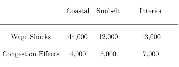
Lower values do not significantly change our estimates. Even with α= 0.1, most of the variation in house prices comes from direct shocks to wages and not from variation
in congestion effects. Lemma 2 shows that we can decompose the variation in house
7As will be seen in the next Section, in order to identify the parameters of the model, we derive
moment conditions from the equation in Lemma 2. More moment conditions than parameters we have to identify are derived. Nevertheless, when we try to simultaneously identify the five parameters (r,
prices from trend as
Ht−Hˆt =xt+
Et(xt+1)
φ−δ
| {z }
wage shocks
− α(1 +r)
1 +r−φ(Nt− ˆ Nt)
| {z }
congestion effects
. (6)
Table 2 lists the volatility of each term using the parameters we estimate for each of the
three regions of the United States (calculation details are in the technical appendix).
In all three cases, wage shocks are much more important than variation in congestion
effects. The value of α is much more important in determining the steady- state (i.e. trend) size of the city, but this steady-state is not our focus here.
The parameterαcombines the impact that extra population has on wage levels with the impact that extra population has on amenities, and we also must use a distinct
estimate of the connection between population and wage levels to correct our wage
series for the change in population. Given the absence of compelling evidence on the links between population size and amenity levels, and the possibility that the link is
actually positive (if access to other people is a consumption amenity), we make the
simplifying assumption that the impact of population on amenities is zero, so that the
value of α is the same as the value of αW. While we do not literally believe this,
assuming it has little impact on our estimates since it only serves to allow us to infer
productivity changes from wage changes by correcting for the changes in population.
As year-to-year population changes are relatively modest, different means of correcting
for population changes have little impact on the inferred productivity series.
In principle all eight parameters in our model could differ across each metropolitan area, but data limitations make it impossible for us to precisely estimate distinct values
for each location. Instead, we assume the calibrated parameters (r,α,w) to be identical for all metropolitan areas and we estimate different values of the parameters (δ, θ, σ, c1, c2) for three different regions of the U.S.8 Our three regions are coastal, sunbelt
and interior. Metropolitan areas whose centroids are within 50 miles of the Atlantic
or Pacific Oceans are defined as coastal. Metropolitan areas more than 50 miles from
either coast and which are in the broad swath of southern and western states on the
southern border of the country running from Florida through Arizona are defined to be
in the sunbelt region. The remainder of our metropolitan areas are defined as being in
the interior region of the country.
8Obtaining different estimates of (r,α,w) for each of these three areas is impossible, as the sources
3.1
Data
For our estimation exercise, we need data on housing prices, construction of new houses, number of households potentially supplying labor, and income per household for a
significant number of metropolitan areas.
The housing price data is based on Federal Housing Finance Agency repeat sales
indices. Construction data are housing permits reported by the U.S. Census. To
esti-mate annual changes in the number of households, we impute the housing stock based
on decadal census estimates of the housing stock and annual permits data. Specifically,
we estimate the housing stock at timet+j to be
Nti+
Pj−1
k=0P ermits
i t+k
P9
k=0P ermitsit+k
Nti+10−Nti,
where Ni
t and Nti+10 are the housing stocks measured during the two closest censuses
in metropolitan area i. Thus, the change in housing stock is partitioned across years based on the observed permitting activity.
Our primary source of income data comes from the Home Mortgage Disclosure
Act (HMDA) files on reported income on mortgage applications. We observe all loan
applicants, not just successful buyers. The HMDA data extend back to 1990. Since
HMDA is essentially a 100 percent sample of everyone who sought a mortgage, the
sample sizes are quite large and we have data for every metropolitan area. Importantly, the HMDA data captures household level income, which is the appropriate level given
our model. The disadvantages of using HMDA income data are a relatively short time
series, the fact that we do not observe those who searched but did not apply for a
mortgage, and that the homebuying decision is endogenous, which can create biases
because the selected sample of people who decide to apply for a loan can differ across
markets or years.
An alternative data source on income is the Bureau of Economic Analysis (BEA)
per capita income measure. It is available beginning in 1980 and for all metropolitan
areas. However, it suffers from a number of drawbacks. First, it is at the individual,
not household, level as its name implies. Households, not individuals, purchase housing units. Hence, in our experimentation with this measure, we translate per capita incomes
into household-levels by multiplying by 2.63, which is the average number of people per
housing unit in our sample of areas in 1990. It also captures the incomes of many
people who have been immobile homeowners for many years may not have much to
do with the advantage that a location brings to the marginal purchaser. In addition,
the incomes of renters are both lower and less volatile than those of owners. Hence,
the BEA series is likely to understate the relevant volatility in local incomes, which is
critical given our purposes.9
While we experimented with both income measures, we believe the advantages of the HMDA series far outweighs its negatives. Hence, we report results using this series
and comment on findings with the BEA data where appropriate.
The sample used in the estimation has 21 sunbelt metropolitan areas, 32 coastal
metropolitan areas, and 60 interior ones. The data for housing prices, construction,
number of households, and borrower income spans the period 1990-2004.
3.2
Methodology
As indicated above, we estimate the parameters (δ, θ, σ, c1, c2) subject to particular
values of (r, α, w). We estimate these five parameters using a sequential two-step Generalized Method of Moments estimator.10 Our two stage procedure estimates our parameters by first using the population-corrected wage series to estimate the housing demand parameters and then using housing price and construction series to identify
the housing supply parameters. More specifically, the parameters (δ, θ, σ) are estimated from an equilibrium equation in the labor market using a two-step GMM estimator.
9Based on data from the New York City Housing and Vacancy Surveys (NYCHVS) from
1978-2002, the income of recent homebuyers increases by $1.29 for every dollar increase in BEA-reported per capita income, while that for renters only rises by $0.47. The NYCHVS only covers one city, but it highlights that the volatility of BEA per capita income is lowered by its incorporation of renter income.
10The details of this estimation method are provided in the Appendix. Hansen (1982) proves
Given these estimates, the parameters (c1, c2) are estimated from the equilibrium
equa-tions for the housing market in Lemma 1 using again a two-step GMM estimator.
3.2.1 Description of Moments
The vector of moments used to estimate (δ, θ, σ) is based on the reduced form re-lationship between productivity per worker and the equilibrium number of workers:
Wi
t = cWti −αWNti. The assumption that xit works entirely through the wage process
allows us to write: Wi
t =wi0+w1at+xit−αWNti, which allows for a city-specific
con-stant and a region-specific time trend in labor demand.11 Using this expression for
wages as well as the assumed value of w, we define our productivity variable, which is wages normalized for changes in the number of workers: Wfti = Wti +αWNti. The
resulting equation is: fWti = w0i +wa1t+xit, where xit follows an ARMA(1,1) process.
The stochastic process for the shocks is therefore
xit=δxit−1 +it+θit−1,
with it independently and identically distributed over time with
E[it|xti, xit−1] = 0, and var[it|xit, xit−1] =σ2.
Using these two restrictions on and data on Wfti, we identify the parameter vector
(δ, θ, σ) through a vector of moments
E[f(Wfi; (δ, θ, σ))] = 0.
The exact functional form of the moment function f(Wfi; (δ, θ, σ)) is contained in the
Appendix. This moment function is based on different moments of the one- period
changes in our productivity measure, ∆fW, and relies on the shocks having mean
zero, being uncorrelated with lagged values ofWfi, and having constant variance.12
11We have tried to allow for city-specific time trends but, given the short length of the time
se-ries available for estimation, this impedes the identification of the remaining parameters of the wage equation.
12As a robustness check, we have also estimated (δ,θ,σ) using a multiple-step estimation procedure.
Given the first stage estimates of the housing demand parameters, (ˆδ, ˆθ, ˆσ2), we
use the equilibrium equations in Lemma 1 to build moment conditions that allow us to
identify the vector (c1,c2). Identification of these two parameters is performed through
the vector of moment conditions:
E[v(Hi, Ni, Ii; (c1, c2))] = 0.
The exact functional form of the moment functionv(Hi, Ni, Ii; (c
1, c2)) also is reported
in the Appendix. This moment function is based on different moments of the deviations
between the vector of housing prices, construction, and number of households and their
steady state levels, (H − H, Ib − I, Nb − Nb). The moments defined by the moment
functionv(Hi, Ni, Ii; (c1, c2)) rely on theshocks having mean zero, being uncorrelated
with lagged values ofNi, and having constant variance.
In order to build the sample analogues of
E[f(Wfi; (δ, θ, σ))] = 0,
E[v(Hi, Ni, Ii; (c1, c2))] = 0,
we use sample moment conditions that pool all the observations across metropolitan
areas and time periods which we assume share the same values of the parameter vector
(δ, θ, σ, c1, c2). Specifically, we build the sample analogue of the moment conditions
aggregating across metropolitan areas within regions and over our entire sample
pe-riod. We pool observations across metropolitan areas, instead of splitting them across
different moment conditions, to increase our sample size. After all, GMM estimators have optimal statistical properties only when the number of observations used in each
moment condition goes to infinity, and the standard errors of our GMM estimates are
valid only asymptotically.
3.3
Estimation Results
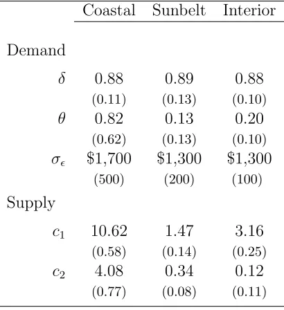
Table 1 reports our estimated parameters. The estimates of the labor demand shocks
persistence parameter, δ, are 0.88 in the interior and coastal areas and 0.89 in the sunbelt. While the similarity of these estimates is striking, they are still somewhat
im-precise. We cannot reject the possibility that income shocks follow a random walk (i.e.,
the persistence parameter equals one) and we also cannot reject much more significant
The estimates of the moving average parameterθ are statistically indistinguishable from zero in the sunbelt and coastal regions. In the interior region, this moving average
component estimate is 0.2 and is marginally significantly different from zero. The
productivity shock estimates range from $1,300 in the sunbelt and interior to $1,700
on the coast. Our estimates of the housing supply parameters reported in the bottom
panel of Table 1 indicate a value for c1 of 10.62 in the coastal region. This implies
that a 1,000 unit increase in the number of building permits in a given year raises the
cost of supplying a home by $10,620. We estimate a value of c2 in that region of 4.08,
meaning that as the number of units in a metropolitan area increases by 10,000 the
cost of supplying a home increases by more than $40,000. The estimates ofc1 are much
lower in the sunbelt and interior regions, at 1.47 and 3.16, respectively. In these two
regions, the estimates ofc2 are 0.34 and 0.12, respectively. Housing supply does appear
to be far more elastic in those regions.13
These latter findings can be compared with the housing supply estimates reported
by Topel and Rosen (1988), who use aggregate national data to estimate an elasticity of housing supply with respect to price that is between 1 and 3. In our model, that
supply elasticity equalsHt/(c1It). In 1990, average prices were about $130,000. Average
construction levels in a metropolitan area is approximately 8,350 units, as measured by
building permits issued. If we take the Topel and Rosen (1988) elasticity to be 3, then
this implies a value ofc1 of 5, which lies in the middle of our estimates.
4
Matching the Data and Discussion
The model presented in Section 2 implies a particular stochastic process process for
housing prices and for the construction of new houses. If shocks are known as they
oc-13As noted above, we generated separate estimates using BEA per capita income data in lieu of
HMDA data. This has the advantage of including years back to 1980, but we also suspect it might grossly underestimate income volatility, which is critical for our purposes. In fact, estimates of the productivity shocks are much lower, with the largest estimate of $1,200 for coastal region markets being smaller that that reported above for sunbelt and interior markets using HMDA data. The moving average parameters are somewhat smaller across all regions, but they are also imprecisely estimated, as was the case with the estimates based on HMDA. The BEA data imply greater differences across regions in the demand shock persistence parameter,δ, with estimates ranging from 0.73 in the interior (and we can reject that coefficient equals one at standard confidence levels) to 0.8 in coastal areas and 0.9 in the sunbelt region. Estimates of supply parameters using BEA per capita income show a very similar pattern to those reported above, albeit with small point estimates. The coastalc1 is 6.1 and
itsc2 is 1.9; those for the interior and sunbelt regions are much closer to zero. See the appendix for
cur, then it is straightforward to show that our model implies the following ARMA(2,3)
process for housing prices, with the parameter vector restricted as outlined in the
ap-pendix:
∆Hti =ai0+a1∆Hti−1+a2∆Hti−2+b0it+b1it−1+b2it−2+b3it−3.
Analogously, the model implies the following ARMA(2,1) process for the construction
of new homes, with the parameter vector restricted as shown in the appendix:
Iti =di0+d1Iti−1+d2Iti−2+e0it−1+e1it−2.
We then use these two ARMA processes, together with the estimated values of the
supply and demand parameters, to derive various predictions of the model over different
time horizons. Certain moments directly estimated from the data are compared to
those analytically derived. In doing so, we focus on a particular set of moments of
these stochastic processes: serial correlations and variances at the one, three and five
year horizons. We do not focus on any contemporaneous or lagged correlations between
prices and quantities for the reasons discussed next, even though much research in
urban and real estate economics uses results from regressions of high frequency prices (or price changes) on demand factors such as income (or income changes).
4.1
The Impact of Information on the Predictions of the Model
The model discussed above assumes that shocks are observed as they occur, but we
are far from confident that they are not known ahead of time. And, the results of
contemporaneous correlations are sensitive to what one assumes about the underlying
information structure (i.e., whether information about the change in income becomes
known ahead of time or only contemporaneously with its public release). In contrast,
autocorrelations of price and construction series are much less sensitive to information
timing as we now demonstrate by comparing the predictions of the model with our
assumed information structure and the predictions if shocks are known one period
ahead of time.
For this exercise, we use parameter estimates from the coastal region: r = 0.04, α = 0.1, c1 = 10.62, c2 = 4.08, θ = 0.82, δ = 0.88, and σ = $1,700. The first column
contemporaneous knowledge.14 The second column represents our model’s predictions
when individuals learn about the income shock one period before it actually impacts
wages.
Advance knowledge slightly increases construction volatility and adds some
momen-tum to house price changes. Otherwise the autocorrelations are essentially unchanged.
Therefore, the predictions of our model for these moments are robust to a possible misspecification of the information structure and a potential lag between the time the
income shocks are known to the agents and when they are made public.
In stark contrast, the impact of the information structure on the contemporaneous
correlation between changes in prices and changes in income is enormous. The bottom
panel of Table 3 shows that if knowledge is contemporaneous to the shock, then the
correlation of price and income changes over short horizons is 0.80. If individuals acquire
knowledge one year ahead, then the predicted correlation is only 0.08. The correlation
is only somewhat more stable at lower frequencies.
Because these correlations are so sensitive to small changes in the underlying in-formation conditions, we focus our analysis on the serial correlation properties and
volatility of price changes and construction activity.15
4.2
Volatility and Serial Correlation in House Prices
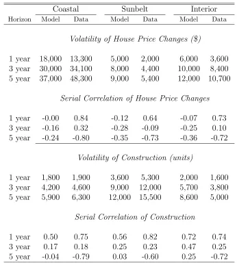
Table 4 documents how well the model matches the data by comparing the model’s
predictions of short- and long-run volatility and serial correlation in house price changes
and new construction with the actual moments from the data. Standard deviations and
serial correlation coefficients from the underlying data over this time period are reported
in columns adjacent to our model predictions.
4.2.1 Volatility in House Prices
The model generally overpredicts price volatility except in the coastal region at 3- and
5-year horizons. One explanation for this excess predicted volatility is that the HMDA
data may be overestimating the actual volatility in local labor demand. Predicted
volatility is closer to the data in both absolute and percentage terms over longer horizons
14For anyj year interval, these predictions reflect the relationship between what happened between
timetandt−j and what happened between timetandt+j.
15Over longer horizons, a one-year shift in when information becomes known is less important, so it
in the interior regions. Those differences are within $2,000. And, the model captures
the sharply rising volatility in price changes over longer horizons in coastal markets,16
but it never matches the very high price volatility seen in those areas over 3- and 5-year
horizons. Except in coastal markets, there appears to be more than enough volatility
in local income processes to account for house price volatility.17
4.2.2 Serial Correlation in House Prices
Turning now to the model predictions about the serial correlation of house price changes
over 1, 3 and 5 year horizons reported in the second panel of Table 4 ,the model predicts
very modest autocorrelation of one- year price changes, ranging from zero in the coastal
region to -0.12 for the sunbelt region. Comparing these predictions with the actual data
reveals a glaring mismatch between the model and reality. In the real world, as Case
and Shiller (1989) documented long ago, there is strong positive serial correlation at one-year frequencies. A one dollar increase in prices during one year is associated with
between a 64 and 84 cent increase in prices during the next period, depending upon
region.
There is no reasonable calibration of the model that can match the strong positive
serial correlation of prices at high frequencies. One possible explanation lies in the
microfoundations of the housing market. If there is a learning process at work, whereby
people gradually infer the state of demand from prices, then this can generate serial
correlation. An alternative explanation is less rational: people see past price changes
and infer future price growth (as in Glaeser, Gyourko and Saiz, 2008). Neither idea is captured in our model. In our model, individuals are fully rational and they know the
parameters that govern the stochastic process for housing prices and construction of
new houses.
At three year periods, the model and the data continue to diverge. The model
con-tinues to predict mean reversion in prices, with the implied serial correlation coefficient
ranging from -0.16 for the coastal region to -0.28 for the sunbelt region. The real data
shows at least mild positive serial correlation for all but the sunbelt region. Once again,
16This is due to the higher underlying volatility in the local income process (σis 30 percent higher
in the coastal metropolitan areas), as well as higher moving average componentθ.
17The results are far different if the BEA income series is used. In that case, the model grossly
price changes are too positively correlated to match the model.
At 5-year time horizons, the model correctly predicts that price changes mean revert,
which is an important stylized fact about local housing markets. However, the point
estimates are well below the amount of mean reversion apparent in the data. This is
one case in which we are skeptical of the data because our procedures for detrending,
which involve subtracting the metro area means, probably induce some spurious mean reversion given the limited fifteen year time series.
While part of the reason for the magnitude mismatch may be due to this factor,
that does not provide a complete explanation. If we lengthen the price change time
series and include the 1980s, computed mean reversion is lower, but is still higher than
our estimates in Table 4 . For example, the serial correlation in five year price changes
falls from - 0.80 to -0.57 in the coastal region. That still is more than double the -0.24
estimate yielded by our model (Table 4). And, using BEA per capita income over the
longer time period dating back to 1980 does not yield a perfect (or close to perfect)
match either.18 Hence, the model should be viewed as successful in capturing the fact that there is mean reversion in price changes over long horizons, but it fails to match
the strength of that pattern.
4.3
Volatility and Serial Correlation in Construction
4.3.1 Volatility in Construction
The model matches the volatility of construction activity at all time horizons in the
coastal region quite well, and especially at high frequency (panel 3, Table 4 ). The
match quality is less good, but tolerable, in the sunbelt region. The model predicts much greater volatility over longer horizons, but underpredicts volatility by one- quarter
to one-third in this region. We consistently overpredict construction quantity by at least
25% at each horizon in interior markets.19
18Similar patterns are evident in the other regions.
19As was the case for price change volatility, using per capita income from the BEA in lieu of
4.3.2 Serial Correlation in Construction
In stark contrast to the model’s complete failure to predict strong persistence in price changes over one-year horizons, it always correctly predicts positive, high frequency
serial correlation in construction in all regions, with the match being very good for the
interior region. Our estimates are about one-third below what the actual data show for
the coastal and sunbelt regions, so complete success for the model cannot be claimed
here. We do better at 3-year horizons. Our model estimates correctly mimic the lower
level of serial correlation at this longer horizon in all regions. And, our point estimates
are very close matches to the data in the coastal and sunbelt regions.
However, the estimates over 5-year horizons do not match the data. As noted above,
we are skeptical of the value of creating such differences using only 15 years of data. If we go back and include the 1980s, calculated mean reversion fall by about two-thirds
in each region (e.g., from -0.79 to -0.27 in the coastal region; from -0.60 to -0.20 in the
sunbelt region; and from -0.72 to -0.24 in the interior region). Thus, it certainly looks
as if the short time span over which we have higher quality income data is leading to an
upwardly biased level of mean reversion in construction for the model to match. That
said, our model estimates still do not match those lower levels of mean reversion.20
5
Conclusion
This paper presents a dynamic linear rational expectations model of housing markets
based on cross-city spatial equilibrium conditions. Its aim is to show how well a housing
model that focuses on income shocks may approximate certain features of the housing
market. The model predicts that housing markets will be largely local, which they are,
and that construction persistence is fully compatible with price mean-reversion. The
model is also consistent with price changes being predictable.
The model has notable successes and failures at fitting the real data. It generally
captures important differences across types of markets, especially coastal ones that have inelastic supply sides to their housing markets. The model also does a decent job of
accounting for variation in price changes. An important implicit assumption underlying
that conclusion is that the HMDA series more accurately reflects the volatility of local
20This is the one case in which using the BEA data on income and the longer time series including the
income processes than (say) the BEA’s per capita income measure. More in-depth
research on this data issue seems warranted given its importance in allowing the model
to approximate market price volatility. This conclusion also generally applies to the
volatility of quantities as reflected in construction permits.
That said, we still cannot precisely match the very high volatility of three- and
five-year price changes observed in the inelastically supplied coastal regions. Thus, it also would be useful for future research to try to pin down whether there is excess volatility
in those markets.
The model does tolerably well at accounting for the strong positive serial correlation
of construction quantities from one year to the next. It also correctly captures the
weakening of this persistence over longer horizons, but fails to match the magnitude of
the mean reversion in quantities over longer horizons especially. Some of the failure in
matching the magnitude of mean reversion in prices and quantities over longer horizons
may be due to data error, but that is not a complete explanation. This is another
avenue for fruitful research.
The model fails utterly at explaining the strong, high frequency positive serial
corre-lation of price changes. It does a much better job of accounting for the mean reversion
over longer, five-year horizons, especially when one takes into account the likelihood
our procedures overstate true mean reversion over this longer time span.
This suggests that housing economists have one very big puzzle to explain, along
with some other issues. The major puzzle is the strong persistence in high frequency
price changes from one year to the next. This failure must be viewed as stark given
that attempt to match moments for a time period that does not include the recent
extraordinary boom and bust. Other matters that certainly merit closer scrutiny include the extremely high price change volatility in coast markets over longer time horizons
and the inability to match mean reversion in construction over longer horizons. These
empirical misses are significant, but it remains true that a dynamic urban model can
account for many of the important features of housing markets. We see this model as a
starting point for a larger agenda of research on real estate dynamics that starts with
a dynamic spatial equilibrium model. One natural extension is to include interest rate
volatility, and we have sketched such an approach in an earlier version of this paper. A
second extension is to relax the assumption of perfect rationality for home-buyers, and
References
Alonso, W. (1964): Location and Land Use. Cambridge, MA: Harvard University
Press.
Andrews, D.(1999): “Estimation When a Parameter Is on a Boundary,”
Economet-rica, 67, 1341-1383.
— (2002): “Generalized Method of Moments Estimation When a Parameter Is on a
Boundary,” Journal of Business and Economics Statistics, 20(4), 530-544.
Arellano, M. and S. Bond. (1991): “Some Tests of Specification for Panel Data:
Monte Carlo Evidence and an Application to Employment Equations,” Review of
Economic Studies, 58(2), 277-97.
Bansal, R., D. Kiku, and A. Yaron(2006): “Risks for the Long Run: Estimation
and Inference,” Working Paper, The Wharton School, University of Pennsylvania.
Blanchard, O. and L. Katz (1992): “Regional Evolutions,” Brookings Papers on
Economic Activity, 1, 1-75.
Borjas, G. (2003): “The Labor Demand Curve Is Downward Sloping: Reexamining
the Impact of Immigration on the Labor Market,” Quarterly Journal of Economics,
188(4), 1335-1374.
Campbell, J. (2000): “Asset Pricing at the Millennium,” Journal of Finance, 60(4),
1515-1567.
Card, D. and K. Butcher (1991): “Immigration and Wages: Evidence from the
1980s,” American Economic Review, 81(2), 292-296.
Case, K. E. and R. Shiller(1989): “The Efficiency of the Market for Single Family
Homes,” American Economic Review, 79(1), 125-37.
Cutler, D., J. Poterba, and L. Summers (1991): “Speculative Dynamics,”
Re-view of Economic Studies, 58(3), 529-46.
Fama, E. and K. French(1988): “Permanent and Temporary Components of Stock
Favilukis, J., S. Ludvigson, and S. Van Nieuwerburgh (2010):
“Macroeco-nomic Effects of Housing Wealth, Housing Finance and Limited Risk Sharing in
General Equilibrium,” Working Paper No. 15988, National Bureau of Economic
Re-search.
Glaeser, E. and J. Gyourko(2005): “Urban Decline and Durable Housing,”
Jour-nal of Political Economy, 113(2) 345-375.
Glaeser, E., J. Gyourko and R. Sacks (2005): “Why Have House Prices Gone
Up?” American Economic Review, 95(2), 329-333.
Gyourko, J., C. Mayer, and T. Sinai(2013): “Superstar Cities,” American
Eco-nomic Journal: EcoEco-nomic Policy, 5(4), 167-199.
Gyourko, J. and A. Saiz (2006): “Construction Costs and the Supply of Housing
Structure,” Journal of Regional Science, 46(4), 661-680.
Hansen, L. (1982): “Large Sample Properties of Generalized Method of Moments
Estimators,” Econometrica, 50, 1029-1054.
Hansen, L. and R. Jagannathan (1991): “Implications of Security Market Data
for Models of Dynamic Economies,” Journal of Political Economy, 99(2), 225-262.
Hendershott, P. and J. Slemrod (1983): “Taxes and the User Cost of
Capi-tal for Owner-Occupied Housing,” Journal of the American Real Estate and Urban
Economics Association, 10(4), 375-93.
Himmelberg, C., C. Mayer and T. Sinai (2005): “Assessing High House Prices:
Bubbles, Fundamentals, and Misperceptions,” Journal of Economic Perspectives,
19(4), 67-92.
Newey, W.(1984): “A Method of Moments Interpretation of Sequential Estimators,”
Economic Letters, 14, 201-206.
Newey, W. and D. McFadden(1994): “Large Sample Estimation and Hypothesis
Testing,” inHandbook of Econometrics, IV, ed. by R. F. Engle and D. L. McFadden.
Polinsky, A. and D. Ellwood(1979): “An Empirical Reconciliation of Micro and
Grouped Estimates of the Demand for Housing,”Review of Economics and Statistics,
61(2), 199-205.
Poterba, J. (1984): “Tax Subsidies to Owner-Occupied Housing: An Asset Market
Approach,” Quarterly Journal of Economics, 99(4), 729-52.
Roback, J. (1982): “Wages, Rents, and the Quality of Life,” Journal of Political
Economy, 90(4), 1257-78.
Rosen, S.(1979): “Wage-Based Indexes of Urban Quality of Life,” in Current Issues
in Urban Economics, ed. by P. Mieszkowski and M. Straszheim. Baltimore: Johns
Hopkins Univerity Press.
Saiz, A.(2003): “Room in the Kitchen for the Melting Pot: Immigration and Rents,”
Review of Economics and Statistics, 85(3), 502-521.
Shiller, R. (2005): Irrational Exuberance (2nd edition). Princeton: Princeton
Uni-versity Press.
— (2006): “Long-Term Perspectives on the Current Boom in Home Prices,” The
Economists’ Voice, 3(4).
Thaler, R.(1978): “A Note on Crime Control: Evidence from the Property Market,”
Journal of Urban Economics, 5(1), 137-145.
Topel, R. and S. Rosen(1988): “Housing Investment in the United States,”Journal
of Political Economy, 96(4), 718-740.
Tracy, J., H. Schneider and S. Chan(1999): “Are Stocks Overtaking Real Estate
in Household Portfolios?,” Current Issues in Economics and Finance, 5(5), 1-6.
Van Nieuwerburgh, S. and P. Weill(2010): “Why Has House Price Dispersion
Gone Up?,” Review of Economic Studies, 77(4), 1567-1606.
Wheaton, W. and G. Nechayev(2008): “The 1998-2005 Housing ‘Bubble’ and the
Current ‘Correction’: What’s Different This Time?” Journal of Real Estate Research
Appendix
Sequential Two-Step GMM Estimator
Let Zti denote a vector of observed variables that correspond to observation i at period t.
This vector may include lagged variables. Denote by ζ the vector of structural parameters
that we want to estimate. In our model, the parameter vectorζ corresponds to (δ, θ, σ, c1, c2).
Specifically, we use ξ to summarize the vector of wage-related housing demand parameters,
(δ, θ, σ), andγ to denote the vector of housing supply parameters (c1, c2).
We split the vector of moment functions provided by the model into a subvector that
de-pends only on the wage-related structural parametersξ,f(Zti;ξ), and the remaining subvector
of moment functions that depends both on ξ and γ, v(Zti;ξ, γ). Therefore, using the set of
moment functionsf(·), we can obtain GMM estimates ofξ that do not depend on the value of
γ, ˆξSEQ. Using the vector of moment functionsv(·) and our estimates of ξ, we then estimate
γ in our second step, ˆγSEQ. These estimates of γ will depend on the values estimated for ξ
in the first step.
We estimate ˆξSEQ by minimizing the objective function:
b Q2(ξ) =
h
(N T)−1
N X i=1 T X t=1
f(Zti;ξ)
i0 c Wf f
h
(N T)−1
N X i=1 T X t=1
f(Zti;ξ)
i .
The weighting matrixWcf f is defined as
c Wf f =
h
(N T)−1
N X i=1 T X t=1
f(Zti; ˆξ1)·f(Zti; ˆξ1)0
i−1 ,
and ˆξ1 minimizes the first stage objective function
b Q1(ξ) =
h
(N T)−1
N X i=1 T X t=1
f(Zti;ξ)i0Ih(N T)−1
N X i=1 T X t=1
f(Zti;ξ)i0,
whereI denotes the identity matrix. Given that this estimate ˆξSEQ does not depend on the
value ofγ, we compute its asymptotic variance as
V ar( ˆξSEQ) =Fbξ0cWf f−1Fbξ −1
whereWcf f is defined above andFbξ is
b
Fξ= (N T)−1 N X i=1 T X t=1 ∂ ∂ξf(Z
i t;ξ).
Using this initial estimate of ξ, we compute an estimate of γ by minimizing the following
objective function:
b
Q2(γ; ˆξSEQ) =
h
(N T)−1
N X i=1 T X t=1
v(Zti;γ,ξˆSEQ)i0Wcvv( ˆξSEQ) h
(N T)−1
N X i=1 T X t=1
v(Zti;γ,ξˆSEQ)i,
whereWcvv( ˆξSEQ) is
c
Wvv( ˆξSEQ) =
h
(N T)−1
N X i=1 T X t=1
v(Zti; ˆγ1,ξˆSEQ)·v(Zti; ˆγ1,ξˆSEQ)0
i−1
and ˆγ1 minimizes the first stage objective function
b
Q1(γ; ˆξSEQ) =
h
(N T)−1
N X i=1 T X t=1
v(Zti;γ,ξˆSEQ)i
0
Ih(N T)−1
N X i=1 T X t=1
v(Zti;γ,ξˆSEQ)i
0 .
The correct formula for the asymptotic variance of ˆγSEQ must account for the fact that its
distribution depends not only on the random vector {Zi
t;∀i, t} but also on the additional
random vector ˆξSEQ. Newey (1984) provides the correct formula for the asymptotic variance
of the second step estimator:
V ar(ˆγSEQ) =
h b
Vγ0Wcvv−1Vbγ i−1
+Vbγ−1Vbξ h
b
FξWcf f−1Fbξ0 i−1
b Vξ0Vb−1
0
γ −Vbγ−1 h
b
VξFbξ−1cWf v+
c WvfFb−1
0 ξ cV0ξ
i b Vγ−10.
Following Newey and McFadden (1994), the sequential GMM estimators belong to the
more general family ofextremumestimators. This guarantees that they are consistent,
asymp-totically normal, and have the asymptotic variance described above.
Moment Conditions
Estimation of Housing Demand Parameters
The vectorial moment condition
is based on the following vector of moment functions:
f(Wfi; (δ, θ, σ)) =
τti
τtifWti−s ∀s≥3
(τti)2−(2θ2−2θ+ 2)σ2 τtiτti−1−(−θ2+ 2θ−1)σ2
τtiτti−2−(−θ)σ2
,
with
τti = ∆Wfti−δ∆Wfti−1−(1−δ)wa1 =it+ (θ−1)it−1−θit−2,
and ∆Wfti = Wfti −Wfti−1. Intuitively, one can think of the random variable τti as close to
(but not exactly) a double-difference of the productivity measureWf. The moment function
f(fWi; (δ, θ, σ)) is based on the expectation, variance, and serial correlation of this double
difference, as well as its covariance with lagged values of the productivity measureWf.
Estimation of Housing Supply Parameters
The vectorial moment condition
E[v(Wfi; (δ, θ, σ))] = 0
is based on the following vector of moment functions:
v(Hi, Ni, Ii; (c1, c2)) =
νti
νtiNti−s ∀s≥1
κit
κi
tNti−s ∀s≥0
(νti)2−( ¯φ+ˆθ)2 ( ¯φ−ˆδ)2 + ˆθ
2
ˆ
σ2
(κi t)2−
(1+r)2(ˆδ+ˆθ)2
(c1)2( ¯φ−ˆδ)2
σ2
,
with
νti = ((Hti−Hbti)−δˆ(Hti−1−Hbti−1) +
α(1 +r) 1 +r−φ
(Nti−Nbti)−δˆ(Nti−1−Nbti−1)
,
κit= ((Iti−Ibti)−δˆ(Iti−1−Ibti−1) + (1−φ)
(Nti−Nbti)−ˆδ(Nti−1−Nbti−1)
.
Intuitively, one can think of the random variables ν and κ as functions of the differences
between the current values of the observable variables (H, I, N) and their steady state values,
ofν and κ, as well as their covariances with lagged values of the number of households, N.
Stochastic Processes Predicted by the Model
If shocks are known as they occur, then our model implies the following ARMA(2,3) process
for housing prices
∆Hti=ai0+a1∆Hti−1+a2∆Hti−2+b0it+b1it−1+b2it−2+b3it−3,
whereai0 denotes a metropolitan area effect, and the parameter vector (a1,a2,b0,b1, b2,b3)
is restricted in the following way:
a1 =φ+δ,
a2 =−φδ,
b0 =
¯
φ+θ
¯
φ−δ,
b1 =
δ+r(δ+θ)−θ(δ+φ)−φ¯(1 +δ+φ) ¯
φ−δ ,
b2 =
φφ¯−θ(1 +r+φ( ¯φ−1)) +δ( ¯φ−1−r+θ+θφ) ¯
φ−δ ,
b3 =φθ.
The model also predicts an ARMA(2,1) process for the construction of new houses:
Iti =di0+d1Iti−1+d2Iti−2+e0it−1+e1it−2,
where di
0 denotes a metropolitan area effect and the parameter vector (d1, d2, e1, e2) is
re-stricted in the following way:
d1=φ+δ,
d2=−φδ,
e0=
(1 +r)(δ+θ)
c1( ¯φ−δ)
,
e1=−
(1 +r)(δ+θ)
c1( ¯φ−δ)
Tables
Table 1: Estimated Demand and Supply Parameters HMDA Income Data, 1990- 2004
Coastal Sunbelt Interior
Demand
δ 0.88 0.89 0.88
(0.11) (0.13) (0.10)
θ 0.82 0.13 0.20
(0.62) (0.13) (0.10)
σ $1,700 $1,300 $1,300
(500) (200) (100)
Supply
c1 10.62 1.47 3.16
(0.58) (0.14) (0.25)
c2 4.08 0.34 0.12
(0.77) (0.08) (0.11)
Notes:δ,θ, andσare the autocorrelation parameter, moving average parameter and residual variance of an ARMA(1,1)
estimated for the component of wages that is not explained by a linear time trend and a metropolitan area-specific constant. c1 denotes the derivative of expected future housing prices with respect to current investment in housing
construction; andc2 denote the derivative of the physical capital cost of building a home with respect to the stock of
Table 2: Relative Volatility of Terms in House Price Equation
Coastal Sunbelt Interior
Wage Shocks 44,000 12,000 13,000
Congestion Effects 4,000 5,000 7,000
Table 3: Sensitivity of Predictions to Different Information Structures
Contemporaneous Knowledge One Horizon Knowledge Year Ahead
Serial Correlation of Construction
1 year 0.51 0.56
3 year 0.18 0.19
5 year -0.04 -0.03
Volatility of Construction (units)
1 year 1,800 2,000
3 year 4,300 4,800
5 year 6,000 6,700
Serial Correlation of House Price Changes
1 year -0.00 0.09
3 year -0.16 -0.10
5 year -0.24 -0.21
Volatility of House Price Changes ($)
1 year 18,000 17,000
3 year 30,000 31,000
5 year 37,000 39,000
Correlation of Income Changes and House Price Changes
1 year 0.80 0.08
3 year 0.93 0.61
5 year 0.95 0.75
Notes: The parameter values estimated for the coastal region using HMDA wage data are assumed here:δ= 0.88,θ= 0.82,σ= $1,700,
Table 4: Volatility and Serial Correlation in House Prices and Construction: HMDA Income Data, 1990-2004
Coastal Sunbelt Interior
Horizon Model Data Model Data Model Data
Volatility of House Price Changes ($)
1 year 18,000 13,300 5,000 2,000 6,000 3,600 3 year 30,000 34,100 8,000 4,400 10,000 8,400 5 year 37,000 48,300 9,000 5,400 12,000 10,700
Serial Correlation of House Price Changes
1 year -0.00 0.84 -0.12 0.64 -0.07 0.73 3 year -0.16 0.32 -0.28 -0.09 -0.25 0.10 5 year -0.24 -0.80 -0.35 -0.73 -0.36 -0.72
Volatility of Construction (units)
1 year 1,800 1,900 3,600 5,300 2,000 1,600 3 year 4,200 4,600 9,000 12,000 5,700 3,800 5 year 5,900 6,300 12,000 15,500 8,600 5,000
Serial Correlation of Construction
1 year 0.50 0.75 0.56 0.82 0.72 0.74 3 year 0.17 0.18 0.25 0.23 0.47 0.25 5 year -0.04 -0.79 0.03 -0.60 0.25 -0.72
Appendix Table 1: Estimated Demand and Supply Parameters: BEA Income Data, 1980-2003
Coastal Sunbelt Interior
δ 0.80 0.90 0.73
(0.11) (0.08) (0.07)
θ 0.16 -0.01 -0.06
(0.13) (0.16) (0.13)
σ $1,200 $1,000 $800
(200) (100) (80)
Supply
c1 6.08 1.00 2.03
(1.21) (0.09) (0.35)
c2 1.88 0.20 0.48
(0.40) (0.03) (0.12)
Notes:δ,θ, andσare the autocorrelation parameter, moving average parameter and residual variance of an ARMA(1,1)
estimated for the component of wages that is not explained by a linear time trend and a metropolitan area-specific constant. c1 denotes the derivative of expected future housing prices with respect to current investment in housing
construction; andc2 denote the derivative of the physical capital cost of building a home with respect to the stock of