Improving the accuracy: volatility modeling and forecasting using high-frequency data and the variational component

(1)

JIEM, 2010 – 3(1): 199-220 – Online ISSN: 2013-0953 Print ISSN: 2013-8423

Improving the accuracy: volatility modeling and forecasting

using high-frequency data and the variational component

Manish Kumar

Department of Management Studies, Indian Institute of Technology Madras (INDIA)

[email protected]

Received September 2009

Accepted February 2010

Abstract:

In this study, we predict the daily volatility of the S&P CNX NIFTY market

index of India using the basic ‘heterogeneous autoregressive’ (HAR) and its variant. In

doing so, we estimated several HAR and Log form of HAR models using different

regressor. The different regressors were obtained by extracting the jump and continuous

component and the threshold jump and continuous component from the realized volatility.

We also tried to investigate whether dividing volatility into simple and threshold jumps and

continuous variation yields a substantial improvement in volatility forecasting or not. The

results provide the evidence that inclusion of realized bipower variance in the HAR models

helps in predicting future volatility.

Keywords: realized volatility, forecasting, time series analysis, autoregressive model

1 Introduction

(2)

interdependent. So both academics and practitioners have emphasised on volatility over the past three decades. Poon and Granger (2003) gave a comprehensive review of the related literature, concentrating on two important questions. Is volatility forecastable? If it is, which method will provide the best forecasts? The authors conclude that financial market volatility is clearly forecastable. However, the debate is on how far ahead one could accurately forecast and to what extent volatility changes could be predicted.

Various statistical and econometrics models are available for forecasting time series volatilities. The simplest one based on historical price is the Random Walk model. The extension of the idea of Random Walk model is the Historical Average method, the simple Moving Average method, the Exponential Smoothing method and the Exponentially Weighted Moving Average (EWMA) method. The Riskmetrics model uses the EWMA method. The second group of models belongs to the regression family. Under which are the Simple Regression, Autoregressive Integrated Moving Average (ARIMA), Autoregressive Fractionally Integrated Moving Average (AFRIMA) and Threshold Autoregressive models (Poon & Granger, 2003).

A third and more sophisticated group of time series models is the ARCH family, extensively used by many researchers. ARCH (Engle, 1982) and GARCH (Bollerslev, 1986) models have been used by many academicians and practitioners, to estimate volatility. They have helped understand empirical properties such as volatility clustering, leverage effects in volatility and fat-tails of many financial time series.

A popular and fourth group for modelling changing volatility persistence is the Hamilton (1989) type regime switching (RS) model. Afterwards, the base RS model was extended by coupling the GARCH type heteroskedasticity in each state and the probability of switching between states to be time dependent. Moreover, a regime switching ARCH with leverage effect and a bivariate RS model was also developed that produced better forecasts (Hamilton & Rauli Susmel, 1994; Hamilton & Gang Lin, 1996).

(3)

In addition to the time series volatility forecasting models, option Implied Standard Deviation (ISD) as a volatility forecast is also used. Lamoureux and Lastrapes (1993) and George Vasilellis and Nigel Meade (1996) in their study found implied ISD predicts equity volatility better than forecasts produced from other time series models.

Various methods for estimating volatility of asset returns also exist. These models and estimators, which assume volatility to be constant, are the oldest ones and they estimate the “unconditional volatility”. Traditional estimates such as standard deviation, close-to-close volatility, extreme value estimator of Parkinson (1980) and Garman and Klass (1980) are examples of unconditional volatility. However, they do not incorporate time-varying characteristics. Work of Engle (1982) on ARCH model led to the development of conditional volatility, which incorporates the time-varying characteristics. Afterwards, many variants of ARCH model have been developed (see Poon & Granger, 2003 and Pandey, 2003).

Robustness of volatility estimates rely severely on the parametric model specification, as well as particular distribution assumptions. An alternative to proxy the volatility is the use of daily squared returns. However, the study by Anderson and Bollerslev (1998) reveals that because of microstructure frictional effects in the dataset, the volatility estimates based on the model-free method can be very noisy. Thus, the estimate based on daily squared returns is not better than the parametric models mentioned before.

Moreover, in a seminal paper, Andersen and Bollerslev (1998) developed a new methodology to estimate the volatility using intraday high frequency returns. They defined this new measure of volatility as Realised Volatility (RV) and proposed to use it as a proxy for the ex-post realisation of the daily volatility. The basic idea of RV is that a reliable measure of the asset volatility can be proxied by the summation of squared returns over the relevant horizon. Anderson and Bollerslev (1998) found that RV furnishes a less noisy estimate than the squared returns to the latent volatility.

(4)

states that RV is a convenient method of circumventing certain data complications, while retaining much of the relevant information within the intraday data for measuring, modelling and forecasting volatility levels over both daily and longer horizons.

Since RV is non-latent, it has not only been used to estimate the predictive performance and adequacy of existing forecasting models (Andersen & Bollerslev, 1998), but also to explore the predictability of RV (Andreou & Ghysels, 2002, Maheu & McCurdy, 2002 , Andersen et al., 2003, Martens et al., 2004, Andersen et

al., 2005, Koopman et al., 2005).

However, the main disadvantage of earlier studies using pure time series specifications of RV is that they ignored the benefits of model averaging and did not include additional volatility proxies, which may be advantageous in increasing the accuracy of the time series forecasting models.

Barndorff-Nielsen and Shephard (2004, 2006) in their research have presented various new measures of volatility and associated estimators. They decomposed the RV into continuous sample path variations and jumps. The authors extended the theory of quadratic variation of semi martingales and provided an asymptotic statistical foundation for this decomposition procedure, under very general conditions. They developed the most popular Realised Power Variation (RPV) and Realised Bipower Variation (RBV). The idea is to examine the role of jumps and continuous component of volatility in volatility forecasting. RPV is built from the sum of powers of the absolute value of high frequency returns, while RBV is defined as the sum of the products of intraday adjacent returns (Barndorff-Nielsen & Shephard, 2004, 2006).

(5)

In a recent study, Corsi et al. (2009) introduced the concept of threshold bipower variation, which is based on the joint use of bipower variation and threshold estimation. Empirical analysis (on the S&P500 index, single stocks and US bond yields) shows that the proposed techniques improve significantly the accuracy of volatility forecasts especially in periods following the occurrence of a jump. In most recent studies (Ghysels et al. (2006), Andersen et al. (2007), and Forsberg & Ghysels (2007)), it has been shown that taking volatility measure which is immune to jumps—that is, RPV or BPV measures—provides a good regressor for predicting future volatility.

In this study, we use the basic HAR-RV and its variant to empirically investigate the dynamic behaviour of the daily RV of the S&P CNX Nifty Index of India. This paper contributes to a growing literature that investigates time series models of RV and their forecasting power in a number of ways. The HAR model proposed by Corsi (2004) and logarithmic version (log-HAR) models are popular methodologies, very successful at modelling the long-term behaviour of volatility in a very simple and parsimonious way. Moreover, while exhibiting good out-of-sample forecasting performance, the HAR-RV model has also been found to substantially outperform several other standard models. The first contribution of the study is to examine whether the use of RBV increases the accuracy volatility forecast. In doing so, we construct RV and RBV at a daily frequency using high frequency intraday observations on returns.

(6)

Although there are studies addressing the issue of forecasting financial time series such as stock market index, most of them are about developed financial markets (UK, US and Japan) but not emerging markets. Nowadays, many international investment bankers and brokerage firms have major stakes in overseas markets. Harvey (1995) found emerging market returns are more likely to be influenced by local information than developed markets; in fact, emerging market returns are generally more predictable than developed market returns, and are more volatile as well. Indian stock markets have received relatively little attention until recently. Now there is more interest and research on Indian market data due to the country’s rapid growth and potential opportunities for investors. Since the establishment of National Stock Exchange (NSE), the financial markets in the world’s second-most populous nation have attracted considerable global investments. It is believed that our investigation using the Indian stock market data would provide a useful assessment of whether the results reported in the earlier studies apply to stock markets in developing nations as well.

The remaining portion of this paper is organized as follows. Section 2, explains the theory of realized volatility, realized power variation and realized bipower variation. The sample period and methodology used for developing and testing the forecasting models are presented in section 3. The experimental results of the study are discussed in section 4. Section 5, concludes with a discussion.

2 Theoretical framework: RV, RBV and jump component extraction

As discussed in Chung et al. (2008) the variation and jump components are extracted as follows. Suppose that, along day t, the logarithmic prices denoted as

Pt

𝑃

𝑡

=

𝑃

0

+

µ

(

𝑡

)

𝑑𝑡

+

𝜎

(

𝑡

)

𝑑𝑤𝑡

+

𝜅

(

𝑡

)

𝑑𝑞

(

𝑡

), 0

≤ 𝑡 ≤ 𝑇

(1)

of a given asset follow a stochastic-volatility process, as

Where μ(t) is a continuous and locally bounded variation process, σ(t) is the stochastic volatility process, W(t) denotes a standard Brownian motion, dq(t) is a counting process with dq(t) = 1 corresponding to a jump at time t and dq(t) = 0 corresponding to no jump and k(t) is the jump size.

(7)

𝑄𝑉𝑡,𝑡+𝐻 =∫_𝑡𝑡+𝐻𝜎2(𝑠)𝑑𝑠+∑𝑡<𝑠<𝑡+𝐻𝜅2(𝑠) (2)

The quadratic variation increments can be decomposed into two distinct components: integrated volatility (continuous) and discrete jumps. Barndorff-Nielsen and Shephard (2004) define integrated power variation of order p as

∫𝑡+𝐻𝜎𝑝_{(𝑠)𝑑𝑠}

𝑡 (3)

, where 0 < p ≤ 2

Although the volatility measures present in equation (2) are unobservable, they can nevertheless be estimated from the data. Let the discrete daily returns be denoted by

𝑟𝑡,𝑡−1=𝑃𝑡− 𝑃𝑡−1, where t refers to daily sampling (4)

The intra-daily return is then

𝑟𝑡𝑀,𝑗 =𝑃𝑡,𝑗/𝑀− 𝑃𝑡,(𝑗−1)/𝑀 (5)

Where M is the number of observations within a trading day.

The daily RV is calculated by summing the corresponding M intra-daily squared returns as

𝑅𝑉

𝑡𝑀,𝑡+1

=

( )

2 1 ,

∑

= M j M j t

r

(6)

According to the quadratic variation theory, the

𝑅𝑉

_𝑡𝑀_,_𝑡+1 will converge uniformly in

probability to the QVt+1

We define RPV and BPV (introduced by Barndorff- Nielsen & Shephard, 2004; 2006) as

with M → ∞.

𝑅𝑃𝑉𝑡𝑀,𝑡+1=

∑

= M j M j t

r

1 , (7)

𝐵𝑃𝑉𝑡𝑀,𝑡+1(𝑘) =µ1−2

∑

+ = M k j M j t

r

1 , M k j t

(8)

Where µ1=�2_𝜋=𝐸(𝑍) denotes the mean of the absolute value of the standard

Gaussian random variable, Z.

It is possible to reveal that for M → ∞

lim𝑀→∞𝑅𝑃𝑉𝑡𝑀,𝑡+1→ ∫_𝑡𝑡+1𝜎(𝑠)𝑑𝑠≡ 𝜎𝑡,𝑡+1 (9)

lim𝑀→∞𝐵𝑃𝑉𝑡𝑀,𝑡+1 → ∫_𝑡𝑡+1𝜎2(𝑠)𝑑𝑠 ≡ 𝜎2𝑡,𝑡+1 (10)

It should be noted that 𝐵𝑃𝑉𝑡𝑀,𝑡+1converges to the continuous path component of the

quadratic variation and is unaffected by jumps.

Combining the results of equations (2) and (8), the quadratic variation process can be separated into the continuous path and jump path components by:

𝑅𝑉𝑡𝑀,𝑡+1− 𝐵𝑃𝑉𝑡𝑀,𝑡+1=

(

)

2

1

s

t s t<

∑

<+

κ

(11)

BPV consistently estimates the integrated variance, even in the presence of jumps.

Thus, the difference between RV and BPV is the sum of the squared jumps. Using the results developed by Barndorff-Nielsen and Shephard (2004, 2006) and Andersen et al. (2007), the significant jumps and the continuous element is defined as

𝐽𝑡𝛼,𝑡+1=𝐼�𝑍𝑡,𝑡+1>𝛷𝛼�(𝑅𝑉𝑡,𝑡+1− 𝐵𝑃𝑉𝑡,𝑡+1)+ (12)

𝐶𝑡𝛼,𝑡+1=𝑅𝑉𝑡,𝑡+1− 𝐽𝑡𝛼,𝑡+1 (13)

Where I(•) denotes the indicator function, and Zt, t +1 is normally distributed

under the null hypothesis of no jumps with a significance level, α, and critical value,

Φα, based on N(0,1) distribution

Similar to Huang and Tauchen (2005), the significance level of the jump test is α =

(9)

Based on a threshold function

Θ

(

M

)

, Mancini (2009) provides alternative

estimators of squared and fourth power integrated volatility. Threshold RV is defined as

𝑇𝑅𝑉𝑡𝑀,𝑡+1=

   

  _≤_Θ =

∑

₍ ₎ 1 2 , 2 , M r M j M j t _M j t

I

r

(14)

Where the threshold functions have to satisfy

lim𝑀→0𝛩(𝑀) = 0, lim𝑀→0𝑀𝑙𝑜𝑔

1 𝑀

𝛩(𝑀) = 0 (15)

Mancini (2009) also establishes a central limit theorem for TRV. Extending the concept, Corsi et al. (2009) developed the threshold multi power variation and threshold bipower variation. He defines threshold bipower variation as

𝑇𝐵𝑃𝑉𝑡𝑀,𝑡+1=𝜇1−2

∑

+ = M k j M j t

r

1 , M k j t

r

,₋

      _≤       _≤ ₋

− j k r j

r tMj M k j t

I

ν

ν , 2

2 ,

(16)

Where 𝜈 is the positive random threshold function.

The jump component is estimated as

𝑇𝐽𝑡𝛼,𝑡+1=𝐼{𝐶−𝑇𝑧>𝛷𝛼}(𝑅𝑉𝑡,𝑡+1− 𝑇𝐵𝑃𝑉𝑡,𝑡+1)+ (17)

And the corresponding continuous part as

𝑇𝐶𝑡𝛼,𝑡+1=𝑅𝑉𝑡,𝑡+1− 𝑇𝐽𝑡𝛼,𝑡+1 (18)

Hence, in this study we employ the concept of RBV and threshold RBV to estimate the jump and continuous component.

3 Data and models

(10)

It is commonly cited in literature (Atchison et al., 1987, Lo & Mackinlay, 1988, Andersen & Bollerslev, 1998) that non-synchronous trading induces serial correlation in the returns process that, in turn, would render the cumulative squared returns measure biased. Moreover, the high frequency data are subjected to the market microstructure effects, due to price discreteness and bid-ask bounces. To remove the effect of microstructure noise and biasness, it is a common practice to sum returns over five or 30 minutes (Andersen et al., (2001, 2005), Barndorff-Nielsen & Shephard, 2004). Hence, in this study, the five-minute returns were constructed using the nearest neighbour to the five–minute tag excluding the overnight returns.

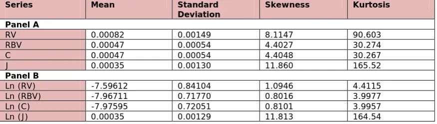
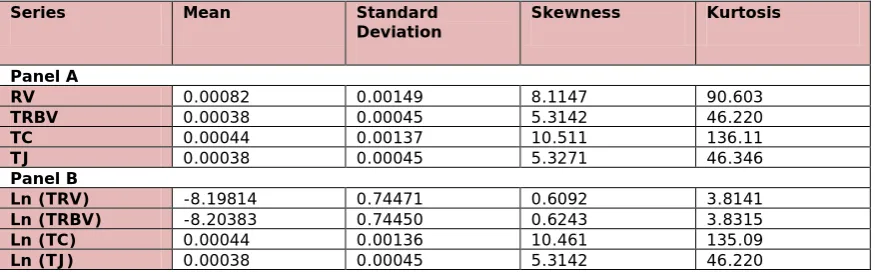
The data is split into two periods. The first period runs from 1 January 2007 to 31 October 2008, used for model estimation and is classified as in-sample; while the second period runs from 1 November 2008 to 15 July 2009, reserved for out-of-sample forecasting and evaluation. Table 1 lists the descriptive statistics of RV levels. These levels include RV, RBV, the continuous element (C) and the jump element (J) and their log-transform. Table 2 shows the descriptive statistics of the threshold bi-power variance, the threshold continuous element (TC) and the threshold jump component (TJ) and their log-transform.

Series Mean Standard

Deviation Skewness Kurtosis

Panel A

RV 0.00082 0.00149 8.1147 90.603

RBV 0.00047 0.00054 4.4027 30.274

C 0.00047 0.00054 4.4048 30.267

J 0.00035 0.00130 11.860 165.52

Panel B

Ln (RV) -7.59612 0.84104 1.0946 4.4115

Ln (RBV) -7.96711 0.71770 0.8016 3.9977

Ln (C) -7.97595 0.72051 0.8101 3.9957

Ln (J) 0.00035 0.00129 11.813 164.54

Table 1. “Descriptive statistics of realized volatility levels”. Source: Own contribution

(11)

transformation of RV, RBV, the C and J. Again the skewness and kurtosis are higher than the standard normal. However, the skewness and kurtosis value have reduced in magnitude compared with the original series.

Series Mean Standard

Deviation Skewness Kurtosis

Panel A

RV 0.00082 0.00149 8.1147 90.603

TRBV 0.00038 0.00045 5.3142 46.220

TC 0.00044 0.00137 10.511 136.11

TJ 0.00038 0.00045 5.3271 46.346

Panel B

Ln (TRV) -8.19814 0.74471 0.6092 3.8141

Ln (TRBV) -8.20383 0.74450 0.6243 3.8315

Ln (TC) 0.00044 0.00136 10.461 135.09

Ln (TJ) 0.00038 0.00045 5.3142 46.220

Table 2. “Descriptive statistics of threshold realized Volatility levels”. Source: Own contribution

Panel A reports the descriptive statistics of the threshold RV and its variants. The values of threshold RBV, the threshold continuous and threshold jump component series are similar to the RV, implying the distribution of these series is also skewed to the right and leptokurtic. Panel B reports the descriptive statistics for the log-transform of the threshold RBV, the threshold continuous and threshold jump component. The values of skewness and kurtosis are higher than the standard normal. However, the skewness and kurtosis value have reduced in magnitude compared with the original series

3.1 Modelling RV–HAR model

(12)

HAR-RV model of Corsi (2004), including the daily, weekly and monthly RV components, is given by

𝐻𝐴𝑅 − 𝑉 − 𝑅𝑉𝑡=𝛼0+𝛼𝑑𝑉𝑡−1+𝛼𝑤𝑉𝑡−5:𝑡−1+𝛼𝑚𝑉𝑡−20:𝑡−1+𝜀𝑡 (19)

Where 𝑉𝑡−ℎ:𝑡=_ℎ+11 (𝑉𝑡−ℎ−1+𝑉𝑡−ℎ+𝑉𝑡) and V=RV, RBV and TRBV

We follow the HAR-RV model introduced by Corsi (2004) and use different repressors such as RV, BPV and TRBV for predicting RV.

In addition to the HAR-RV model, we also use the following model suggested by Chung et al. (2008).

𝐻𝐴𝑅 − 𝐶𝐽 − 𝑅𝑉𝑡=𝛽0+𝛽𝑐𝑑𝐶𝑡−1+𝛽𝑐𝑤𝐶𝑡−5:𝑡−1+𝛽𝑐𝑚𝐶𝑡−20:𝑡−1+𝛽𝑗𝑑𝐽𝑡−1+𝛽𝑗𝑤𝐽𝑡−5:𝑡−1+𝛽𝑗𝑚𝐽𝑡−20:𝑡−1+𝜀𝑡

(20)

Where Ct-h and Jt-h

We use the continuous and jump component elements of RV, as separated by the jump test of Barndorff-Nielsen and Shephard (2006).

are the continuous and jump component respectively.

We modify the HAR-CJ-RV model of Chung et al. (2008) using the continuous and jump component of RV as separated by the jump test of Corsi et al. (2009) using threshold RBV measure.

𝐻𝐴𝑅 − 𝑇𝐶𝐽 − 𝑅𝑉𝑡=𝛽0+𝛽𝑐𝑑𝑇𝐶𝑡−1+𝛽𝑐𝑤𝑇𝐶𝑡−5:𝑡−1+𝛽𝑐𝑚𝑇𝐶𝑡−20:𝑡−1+𝛽𝑗𝑑𝑇𝐽𝑡−1+

𝛽𝑗𝑤𝑇𝐽𝑡−5:𝑡−1+𝛽𝑗𝑚𝑇𝐽𝑡−20:𝑡−1+𝜀𝑡 (21)

Where TCt-h and TJt-h

As suggested by Andersen et al. (2007) and Forsberg and Ghysels (2007) and Chung et al. (2008), we also model RV using log-transform. The logarithmic forms of the above equations are as follows:

are the continuous and jump component respectively.

𝐻𝐴𝑅 − 𝑉 − 𝐿𝑜𝑔𝑅𝑉𝑡=𝛼0+𝛼𝑑𝐿𝑜𝑔𝑉𝑡−1+𝛼𝑤𝐿𝑜𝑔𝑉𝑡−5:𝑡−1+𝛼𝑚𝐿𝑜𝑔𝑉𝑡−20:𝑡−1+𝜀𝑡 (22)

(13)

𝐻𝐴𝑅 − 𝐶𝐽 − 𝐿𝑜𝑔𝑅𝑉𝑡= 𝛽0+𝛽𝑐𝑑𝐿𝑜𝑔𝐶𝑡−1+𝛽𝑐𝑤𝐿𝑜𝑔𝐶𝑡−5:𝑡−1+𝛽𝑐𝑚𝐿𝑜𝑔𝐶𝑡−20:𝑡−1+

𝛽𝑗𝑑𝐿𝑜𝑔𝐽𝑡−1+𝛽𝑗𝑤𝐿𝑜𝑔𝐽𝑡−5:𝑡−1+𝛽𝑗𝑚𝐿𝑜𝑔𝐽𝑡−20:𝑡−1+𝜀𝑡 (23)

Where Ct-h and Jt-h

𝐻𝐴𝑅 − 𝑇𝐶𝐽 − 𝑅𝑉𝑡=𝛽0+𝛽𝑐𝑑𝐿𝑜𝑔𝑇𝐶𝑡−1+𝛽𝑐𝑤𝐿𝑜𝑔𝑇𝐶𝑡−5:𝑡−1+ 𝛽𝑐𝑚𝐿𝑜𝑔𝑇𝐶𝑡−20:𝑡−1+

𝛽𝑗𝑑𝐿𝑜𝑔𝑇𝐽𝑡−1+𝛽𝑗𝑤𝐿𝑜𝑔𝑇𝐽𝑡−5:𝑡−1+𝛽𝑗𝑚𝐿𝑜𝑔𝑇𝐽𝑡−20:𝑡−1+𝜀𝑡 (24) are the continuous and jump components, respectively, as separated by the jump test of Barndorff-Nielsen and Shephard (2006)

Where TCt-h and TJt-h

3.2 Measure of performance

are continuous and jump components, respectively, as separated by the jump test of Corsi et al. (2009)

Following Forsberg and Ghysels (2007) and Chung et al. (2008) the prediction performance of the various models in this study is evaluated by considering mean square error (MSE), mean absolute error (MAE) and mean absolute percentage error (MAPE). However, Andersen et al. (2007) in their study compared the results

of the different models using only adjusted R2_{. Forsberg and Ghysels (2007)}

suggested that, when transformed variable (such as log or square root) are used as

dependent variable, adjusted R2

4 Empirical results

can not be used to compare different models. Hence, it is necessary to recover the transformed variable in its original form using suitable measure. Thus, after recovering the dependent variable to its original form, we have compared the in-sample and out-of-sample of different models using MSE, MAE and MAPE.

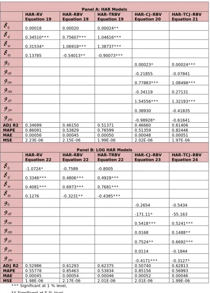
4.1 In-sample results

All the daily forecasting models are estimated using in-sample data which runs from

1st_{January 2007-31}st_{October 2008. The results of the estimation of HAR and the}

(14)

Panel A: HAR Models HAR-RV

Equation 19 HAR-RBV Equation 19 HAR-TRBV Equation 19 HAR-CJ-RBV Equation 20 HAR-TCJ-RBV Equation 21

0

α

_0.00018 _0.00020 _0.00024**

d

α

_0.34510*** _0.75607*** _1.04616***

w

α

_0.31534* _1.06918*** _1.38737***

m

α

_0.13785 _-0.54013** _-0.90073***

0

β

0.00023* 0.00024***

cd

β

-0.21855 -0.07841

cw

β

0.77883*** 1.08498***

cm

β

-0.34119 0.27131

jd

β

1.54556*** 1.32193***

jw

β

0.38930 -0.41835

jm

β

-0.98928* -0.61641

ADJ R2 0.34699 0.46150 0.51371 0.46660 0.61406

MAPE 0.86091 0.53829 0.76599 0.51359 0.82446

MAE 0.00056 0.00045 0.00050 0.00048 0.00051

MSE 2.23E-06 2.15E-06 1.99E-06 2.02E-06 1.97E-06

Panel B: LOG HAR Models HAR-RV

Equation 22 HAR-RBV Equation 22 HAR-TRBV Equation 22 HAR-CJ-RBV Equation 23 HAR-TCJ-RBV Equation 24

0

α

_-1.0724* _-0.7589 _-0.8005

d

α

_0.3346*** _0.4806*** _0.4929***

w

α

_0.4081*** _0.6973*** _0.7681***

m

α

_0.1276 _-0.3231** _-0.4385***

0

β

-0.2654 -0.5434

cd

β

-171.11* -55.163

cw

β

0.5418*** 0.5241***

cm

β

0.0168 0.1488**

jd

β

0.7524** 0.6692***

jw

β

0.0114 -0.1844

jm

β

-0.4171*** -0.3127*

ADJ R2 0.52986 0.61293 0.62375 0.50740 0.62813

MAPE 0.55778 0.85463 0.53834 0.85156 0.56993

MAE 0.00045 0.00054 0.00046 0.00052 0.00046

MSE 1.98E-06 2.17E-06 2.01E-06 2.01E-06 1.99E-06

*** Significant at 1 % level, ** Significant at 5 % level, * Significant at 10 % level

(15)

The results for the coefficient of the HAR (equation 19-21) and LOG-HAR (equation 22-24) model in Panel A and B suggests, RBV and the TRBV is the best regressor in the HAR and transformed Log HAR specification (equation 19 and 22). The daily, weekly and monthly coefficients of RBV and TRBV are significant at 1 % level. This confirms the existence of highly persistent volatility dependence.

The coefficient (daily, weekly and monthly) of jump and continuous component as extracted using by Barndorff-Nielsen and Shephard (2004, 2006) and Corsi et al. (2009) are not significant in many cases (equation 20, 21, 23 and 24). The results also show that only the daily jump coefficient is positive and significant at 1 % level. This suggests that the daily jump may play a role in future volatility forecast.

The results presented in Panel A and B also gives the adjusted R2_{values for the}

HAR and the LOG HAR models. It is noticed that the adjusted R2

In the earlier subsection, we discussed that adjusted R

is higher for the LOG HAR model which also confirms the findings of (Andersen et al. (2007) and Forsberg and Ghysels (2007) and Chung et al. (2008).

2

A glance at the values of these performance measures suggests that no model emerges as winner in the in-sample data. The forecasting accuracy statistics provide very inconclusive results. The MSE measure suggests that an equation 19 (HAR-TRBV) models is the best, while the two other performance measure i.e. MAE and MAPE suggests that the HAR-RV (equation 19) and HAR-CJ-RBV (equation 20) are the best.

cannot be used to compare different models. Hence, we resort to the various error measures to compare the in-sample performance of the RV forecasting model. The study use three error measure namely, MAE, MAPE and MSE to compare various models.

(16)

emphasis on MSE rather than MAE and MAPE. Thus, from an MSE perspective, the HAR-TRBV model is found to provide the best predictions in the in-sample period. The HAR-TRBV model exploits the use of threshold realized bipower variation et al. (Corsi (2009)) to develop the HAR model.

4.2 Out-of-sample results

In order to compare the true performance of the forecasting models, it is necessary to evaluate them on previously unseen data. This situation is likely to be the closest to a true forecasting. To achieve this, all models were maintained with an identical out-of-sample period allowing a direct comparison of their forecasting accuracy. The predictive performance of the five models is summarized in Table 4.

Panel A: HAR Model HAR-RV

Equation 19 Equation 19 HAR-RBV Equation 19 HAR-TRBV HAR-CJ-RBV Equation 20 HAR-TCJ-RBV Equation 21

MAPE 0.92107 0.54698 0.85209 0.55539 0.98982

MAE 0.00057 0.00044 0.00052 0.00044 0.00056

MSE 4.39E-06 3.92E-06 3.98E-06 4.42E-06 4.10E-06

Panel B: LOG HAR Models HAR-RV

Equation 22 Equation 22 HAR-RBV Equation 22 HAR-TRBV HAR-CJ-RBV Equation 23 HAR-TCJ-RBV Equation 24

MAPE 0.67625 1.06432 0.62164 1.08352 0.70795

MAE 0.00048 0.00063 0.00047 0.00061 0.00050

MSE 3.98E-06 3.93E-06 3.97E-06 3.97E-06 3.99E-06

Table 4: “Out-of-Sample Prediction Accuracy”. Source: Own contribution

The forecasting accuracy statistics provide very interesting results. A glance at these values shows the superiority of HAR-RBV i.e. Equation 19 with realized bipower variance as regressor. MAE, MSE and MAPE achieved by the HAR-RBV model are quite low indicating that there is a smaller deviation between the actual and predicted. Ghysels et al. (2006) and Forsberg and Ghysels (2007) in their study concluded that the choice of regressor is clearly more important than either the model or the weighting scheme selected for use. The results provided by the HAR-RBV models suggest that realized bipower variance has contributed more in terms of capturing the fluctuations in future volatility.

The results of our study suggests that HAR models involving RBV are invariant to jumps (Barndorff-Nielsen and Shephard (2004, 2006)) and threshold jumps (Corsi

et al. 2009)), which implies that, even with the presence of a jump at time t , there

(17)

Ghysels (2007) and Chung et al. (2008) but contradict the findings of Corsi et al. (2009). Thus, the out-of-sample performance measures clearly indicate that RBV based HAR model is the best model in terms of forecasting future volatility.

5 Conclusion

In this study, we investigated the volatility of the daily of S&P CNX Nifty Index realized volatility. We tried to examine whether dividing volatility into jumps and continuous variation yields a substantial improvement in volatility forecasting or not. In doing so, we estimated several HAR and Log form of HAR models using different regressor. The study contributes to the existing literature by comparing the performance of different HAR models and Log HAR models with regressor extracted from the Barndorff-Nielsen and Shephard (2004, 2006) and Corsi (2009) methodology. The experimental results obtained using Nifty data show that RBV is the preferred regressor for future volatility prediction. These results hold good for both the in-sample and out-of-sample data. The findings of our study are consistent with the results of Ghysels et al. (2006) and Forsberg and Ghysels (2007) and Chung et al. (2008) but contradict the results of Corsi et al. (2009).

Traders can develop models using HAR-RBV to forecast the RV and use them for better investment decision making. Policy makers can explore the use of such model in predicting realized volatility and examine the impact on other economic indicators of the country.

(18)

Acknowledgement

The author would like to thank Davide Pirino (Dipartimento di Fisica,Universit`a di Pisa), Huimin Chung (National Chiao Tung University), Chin-Sheng Huang and Tseng-Chan Tseng (National Yunlin University of Science and Technology) for sharing their research stuff. The author would like to thank the anonymous reviewers for going through the manuscript patiently and critically and sharing his/her views in improving the article.

References

Andrew, W. L., & MacKinlay, A. C. (1988). Stock Market Prices do not Follow Random Walks: Evidence from a Simple Specification Test. Review of Financial

Studies, 1(1), 41-66.

Andersen, T. G., Bollerslev, T., & Meddahi, N. (2005) Correcting the errors: volatility forecast evaluation using high-frequency data and realized volatilities.

Econometrica, 73(1), 279-296.

Andersen, T. G., Bollerslev, T., Diebold, F. X., & Labys, P. (2003). Modeling and forecasting realized volatility. Econometrica, 71(2), 579-625.

Andersen, T. G., Bollerslev, T., & Diebold, F. X. (2007a). Roughing it up: Including jump components in the measurement, modeling and forecasting of return volatility. Review of Economics and Statistics, 89, 701–720.

Andersen, T. G., Bollerslev, T., & Dobrev, D. (2007b). No-arbitrage semi-martingale restrictions for continuous time volatility models subject to leverage effects, jumps and iid noise: Theory and testable distributional implications. Journal of

Econometrics, 138 (1), 125–180.

Andersen, T. G., Bollerslev, T., Diebold, F. X., & Ebens, H. (2001a). The Distribution of Realized Stock Return Volatility. Journal of Financial Economics, 61, 43-76.

(19)

Andersen, T. G., Bollerslev, T., Diebold, F. X., & Labys, P. (2001b). The Distribution of Realized Exchange Rate Volatility. Journal of the American Statistical

Association, 96, 42-55.

Andersen, T. G., & Bollerslev, T. (1998). Answering the skeptics: Yes, standard volatility models do provide accurate forecasts. International Economic Review,

39, 885-905.

Andreou, E. & Ghysels, E. (2002). Rolling-sample volatility estimators: some new theoretical, simulation, and empirical results. Journal of Business and Economic

Statistics, 20(3), 363-76.

Atchison, M. D., Butler, K. C., & Simonds, R. R. (1987). Nonsynchronous Security Trading and Market Index Autocorrelation. Journal of Finance, 42(1), 111-18.

Barndorff-Nielsen, O.E., & Shephard, N. (2004). Power and Bi-power Variation with Stochastic Volatility and Jumps. Journal of Financial Econometrics, 2, 1-37.

Barndorff-Nielsen, O.E., & Shephard, N. (2002a). Econometric Analysis of Realized Volatility and its Use in Estimating Stochastic Volatility Models. Journal of the

Royal Statistical Society, 64: 253-80.

Barndorff-Nielsen, O.E., & Shephard, N. (2002b). Estimating Quadratic Variation Using Realized Variance. Journal of Applied Econometrics, 17, 457-78.

Barndorff-Nielsen, O.E., & Shephard, N. (2006). Econometrics of Testing for Jumps in Financial Economics Using Bi-power Variation. Journal of Financial

Econometrics, 4, 1-30.

Bates, J. M., & Granger, C. W. J. (1969). The Combination of Forecasts. Operation

Research Quarterly, 20, 451–468.

Bollerslev, T. & Zhou. H. (2002). Estimating stochastic volatility diffusion using conditional moments of integrated volatility. Journal of Econometrics, 109(1),

(20)

Bollerslev, T. (1986). Generalized autoregressive conditional heteroscedasticity.

Journal of Econometrics, 31, 307–327.

Bollerslev, T., Kretschmer, U., Pigorsch, C., & Tauchen, G. (2005). A discrete-time model for daily S&P 500 returns and realized variations: Jumps and leverage effects. Journal of Econometrics.

Brooks, C. (1998). Predicting stock index volatility: can market volume help?

Journal of Forecasting, 17, 59–80.

Corsi, F. (2004). A Simple Long Memory Model of Realized Volatility. Manuscript.

Corsi, F., Pirinos, D. & Ren, R. (2009). Threshold Bipower Variation and the Impact of Jumps on Volatility Forecasting. Working paper at Dipartimento di Economia Politica, Università di Siena.

Engle, R. F. (1982). Autoregressive conditional heteroscedasticity with estimator of the variance of United Kingdom inflation. Econometrica, 50(4), 987–1008.

Fleming, J., Kirby, C., & Ostdiek, B. (2003). The economic value of volatility timing using‘realized volatility. Journal of Financial Economics, 67, 473-509.

Forsberg, L., & Ghysels, E. (2007). Why Do Absolute Returns Predict Volatility So

Well? Journal of Financial Econometrics, 5, 31-67.

Garman, M. B. & Klass, M. J. (1980). On the estimation of Security Price Volatilities

from Historical data. Journal of Business, 53, 67-78.

Ghysels, E., Sinko, A., & Valkanov, R. (2007). MIDAS Regressions: Further Results and New Directions. Econometric Reviews, 26, 53-90.

Ghysels, E., Harvey, A., & Renault, E. (1996). “Stochastic Volatility” in Handbook of

Statistics: Statistical Methods in Finance, 14, G.S. Maddala and C.R. Rao, eds.

(21)

Hamilton, J. D., & Lin, G. (1996). Stock Market Volatility and the Business Cycle.

Journal of Applied Econometrics, 11(5), 573–93.

Hamilton, J. D., & Susmel, R. (1994). Autoregressive Conditional Heteroskedasticity and Changes in Regime. Journal of Econometrics, 64(1–2), 307–33.

Hamilton, J. D. (1989). A New Approach to the Economic Analysis of Nonstationary Time Series and the Business Cycle. Econometrica, 57, 357–84.

Harvey, C. R. (1995). The Risk Exposure of Emerging Equity Markets. World Bank

Economic Review, 9, 19–50.

Huimin, C., Chin-Sheng, H., & Tseng-Chan, T. (2008). Modeling and Forecasting of Realized Volatility Based on High- Frequency Data: Evidence from Taiwan, International Research Journal of Finance and Economics.

Koopman, S. J., Jungbacker, B., & Hol. E. (2005). Forecasting daily variability of the S&P 100 stock index using historical, realised and implied volatility measurements. Journal of Empirical Finance, 12(3), 445-475.

Lamoureux, C., &Lastrapes, W. (1993). Forecasting Stock-Return Variance: toward an Understanding of Stochastic Implied Volatilities. Revue of Financial Studies,

6(2), 293–326.

Maheu, J. M. & McCurdy, T. H. (2002). Nonlinear Features of Realized FX Volatility.

The Review of Economics and Statistics, 84(4), 668-681.

Mancini, C. (2009). Non-parametric threshold estimation for models with stochastic diffusion coefficient and jumps. Scandinavian Journal of Statistics, 36(2), 270–

296.

Martens, M., van Dijk, D. J. C., & de Pooter, M. (2004). Modeling and forecasting

(22)

Pandey, A. (2003). Modeling and Forecasting Volatility in Indian Capital Markets, No 2003-08-03, IIMA Working Papers from Indian Institute of Management Ahmedabad, Research and Publication Department.

Parkinson, M. (1980). The extreme value method for estimating the variance of the

rate of return. Journal of Business, 53, 61-65.

Patton, A. (2006). Volatility Forecast Comparison Using Imperfect Volatility Proxies. Manuscript, London School of Economics

Poon, S., & Granger, C. W. R. (2003). Forecasting Volatility in Financial Markets: A Review. Journal of Economic Literature, 66, 478-539.

Reid, D.J. (1968). Combining Three Estimates ff Gross Domestic Product.

Economica, 35, 431–444.

Tae Hyup, R. (2007). Forecasting the volatility of stock price index. Expert Systems

with Applications, 33 (4), 916-922.

Vasilellis, G. A. & Meade, N. (1996). Forecasting Volatility for Portfolio Selection.

Journal of Business and Financial Accounting, 23(1), 125–143.

Article's contents are provided on a Attribution-Non Commercial 3.0 Creative commons license. Readers are allowed to copy, distribute and communicate article's contents, provided the author's and Journal of Industrial Engineering and Management's names are included. It must not be used for commercial purposes. To see the complete

license contents, please visi