Matlab Primer Highlighted

Primer

Technical Support

[email protected] Product enhancement suggestions [email protected] Bug reports

[email protected] Documentation error reports

[email protected] Order status, license renewals, passcodes [email protected] Sales, pricing, and general information

508-647-7000 (Phone)

508-647-7001 (Fax)

The MathWorks, Inc.

3 Apple Hill Drive

Natick, MA 01760-2098

For contact information about worldwide offices, see the MathWorks Web site.

MATLAB®_Primer

© COPYRIGHT 1984–2012 by The MathWorks, Inc.

The software described in this document is furnished under a license agreement. The software may be used or copied only under the terms of the license agreement. No part of this manual may be photocopied or reproduced in any form without prior written consent from The MathWorks, Inc.

FEDERAL ACQUISITION: This provision applies to all acquisitions of the Program and Documentation by, for, or through the federal government of the United States. By accepting delivery of the Program or Documentation, the government hereby agrees that this software or documentation qualifies as commercial computer software or commercial computer software documentation as such terms are used or defined in FAR 12.212, DFARS Part 227.72, and DFARS 252.227-7014. Accordingly, the terms and conditions of this Agreement and only those rights specified in this Agreement, shall pertain to and govern the use, modification, reproduction, release, performance, display, and disclosure of the Program and Documentation by the federal government (or other entity acquiring for or through the federal government) and shall supersede any conflicting contractual terms or conditions. If this License fails to meet the government’s needs or is inconsistent in any respect with federal procurement law, the government agrees to return the Program and Documentation, unused, to The MathWorks, Inc.

Trademarks

MATLAB and Simulink are registered trademarks of The MathWorks, Inc. See

www.mathworks.com/trademarksfor a list of additional trademarks. Other product or brand

names may be trademarks or registered trademarks of their respective holders.

Patents

MathWorks products are protected by one or more U.S. patents. Please see

July 2002 Online only Revised for MATLAB 6.5 (Release 13) August 2002 Fifth printing Revised for MATLAB 6.5

June 2004 Sixth printing Revised for MATLAB 7.0 (Release 14) October 2004 Online only Revised for MATLAB 7.0.1 (Release 14SP1) March 2005 Online only Revised for MATLAB 7.0.4 (Release 14SP2) June 2005 Seventh printing Minor revision for MATLAB 7.0.4 (Release 14SP2) September 2005 Online only Minor revision for MATLAB 7.1 (Release 14SP3) March 2006 Online only Minor revision for MATLAB 7.2 (Release 2006a) September 2006 Eighth printing Minor revision for MATLAB 7.3 (Release 2006b) March 2007 Ninth printing Minor revision for MATLAB 7.4 (Release 2007a) September 2007 Tenth printing Minor revision for MATLAB 7.5 (Release 2007b) March 2008 Eleventh printing Minor revision for MATLAB 7.6 (Release 2008a) October 2008 Twelfth printing Minor revision for MATLAB 7.7 (Release 2008b) March 2009 Thirteenth printing Minor revision for MATLAB 7.8 (Release 2009a) September 2009 Fourteenth printing Minor revision for MATLAB 7.9 (Release 2009b) March 2010 Fifteenth printing Minor revision for MATLAB 7.10 (Release 2010a) September 2010 Sixteenth printing Revised for MATLAB 7.11 (R2010b)

April 2011 Online only Revised for MATLAB 7.12 (R2011a) September 2011 Seventeenth printing Revised for MATLAB 7.13 (R2011b)

March 2012 Eighteenth printing Revised for Version 7.14 (R2012a)(Renamed from

Quick Start

1

Product Description

. . . .

1-2 Key Features

. . . .

1-2

Desktop

. . . .

1-3

Matrices and Arrays

. . . .

1-6 Array Creation

. . . .

1-6 Matrix and Array Operations

. . . .

1-7 Concatenation

. . . .

1-9 Complex Numbers

. . . .

1-10

Array Indexing

. . . .

1-11

Workspace

. . . .

1-13

Character Strings

. . . .

1-15

Functions

. . . .

1-17

Plots

. . . .

1-18 Line Plots

. . . .

1-18 3-D Plots

. . . .

1-21 Subplots

. . . .

1-22

Scripts

. . . .

1-24 Sample Script

. . . .

1-24 Loops and Conditional Statements

. . . .

1-25 Script Locations

. . . .

1-27

Matrices and Magic Squares

. . . .

2-2 About Matrices

. . . .

2-2 Entering Matrices

. . . .

2-4 sum, transpose, and diag

. . . .

2-5 The magic Function

. . . .

2-7 Generating Matrices

. . . .

2-8

Expressions

. . . .

2-10 Variables

. . . .

2-10 Numbers

. . . .

2-11 Matrix Operators

. . . .

2-12 Array Operators

. . . .

2-13 Functions

. . . .

2-15 Examples of Expressions

. . . .

2-16

Entering Commands

. . . .

2-18 The format Function

. . . .

2-18 Suppressing Output

. . . .

2-19 Entering Long Statements

. . . .

2-20 Command Line Editing

. . . .

2-20

Indexing

. . . .

2-21 Subscripts

. . . .

2-21 The Colon Operator

. . . .

2-22 Concatenation

. . . .

2-23 Deleting Rows and Columns

. . . .

2-24 Scalar Expansion

. . . .

2-25 Logical Subscripting

. . . .

2-26 The find Function

. . . .

2-27

Linear Algebra

. . . .

3-2 Matrices in the MATLAB Environment

. . . .

3-2 Systems of Linear Equations

. . . .

3-11 Inverses and Determinants

. . . .

3-22 Factorizations

. . . .

3-26 Powers and Exponentials

. . . .

3-34 Eigenvalues

. . . .

3-37 Singular Values

. . . .

3-40

Operations on Nonlinear Functions

. . . .

3-44 Function Handles

. . . .

3-44 Function Functions

. . . .

3-44

Multivariate Data

. . . .

3-47

Data Analysis

. . . .

3-48 Introduction

. . . .

3-48 Preprocessing Data

. . . .

3-48 Summarizing Data

. . . .

3-54 Visualizing Data

. . . .

3-58 Modeling Data

. . . .

3-71

Graphics

4

About Mesh and Surface Plots

. . . .

4-16 Visualizing Functions of Two Variables

. . . .

4-16

Plotting Image Data

. . . .

4-23 About Plotting Image Data

. . . .

4-23 Reading and Writing Images

. . . .

4-24

Printing Graphics

. . . .

4-25 Overview of Printing

. . . .

4-25 Printing from the File Menu

. . . .

4-25 Exporting the Figure to a Graphics File

. . . .

4-26 Using the Print Command

. . . .

4-26

Working with Handle Graphics Objects

. . . .

4-28 Graphics Objects

. . . .

4-28 Setting Object Properties

. . . .

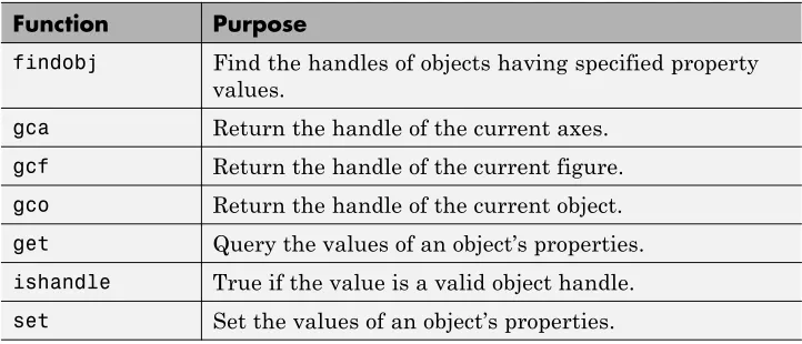
4-30 Functions for Working with Objects

. . . .

4-33 Specifying Axes or Figures

. . . .

4-34 Finding the Handles of Existing Objects

. . . .

4-36

Programming

5

Control Flow

. . . .

5-2 Conditional Control — if, else, switch

. . . .

5-2 Loop Control — for, while, continue, break

. . . .

5-5 Program Termination — return

. . . .

5-7 Vectorization

. . . .

5-8 Preallocation

. . . .

5-8

Quick Start

• “Product Description” on page 1-2

• “Desktop” on page 1-3

• “Matrices and Arrays” on page 1-6

• “Array Indexing” on page 1-11

• “Workspace” on page 1-13

• “Character Strings” on page 1-15

• “Functions” on page 1-17

• “Plots” on page 1-18

• “Scripts” on page 1-24

Product Description

The Language of Technical Computing

MATLAB®_{is a high-level language and interactive environment that enables}

you to perform computationally intensive tasks faster than with traditional programming languages such as C, C++, and Fortran.

Key Features

• High-level language for technical computing

• Development environment for managing code, files, and data

• Interactive tools for iterative exploration, design, and problem solving

• Mathematical functions for linear algebra, statistics, Fourier analysis,

filtering, optimization, and numerical integration

• 2-D and 3-D graphics functions for visualizing data

• Tools for building custom graphical user interfaces

• Functions for integrating MATLAB based algorithms with external

Desktop

When you start MATLAB, the desktop appears in its default layout.

The desktop includes these panels:

• Current Folder— Access your files.

• Command Window— Enter commands at the command line, indicated

by the prompt (>>).

• Workspace— Explore data that you create or import from files.

• Command History— View or rerun commands that you entered at the

command line.

As you work in MATLAB, you issue commands that create variables and call functions. For example, create a variable namedaby typing this statement

at the command line:

MATLAB adds variableato the workspace and displays the result in the

Command Window.

a =

1

Create a few more variables.

b = 2

b =

2

c = a + b

c =

3

d = cos(a)

d =

0.5403

When you do not specify an output variable, MATLAB uses the variableans,

short foranswer, to store the results of your calculation.

sin(a)

ans =

0.8415

If you end a statement with a semicolon, MATLAB performs the computation, but suppresses the display of output in the Command Window.

You can recall previous commands by pressing the up- and down-arrow keys,

Matrices and Arrays

In this section...

“Array Creation” on page 1-6

“Matrix and Array Operations” on page 1-7 “Concatenation” on page 1-9

“Complex Numbers” on page 1-10

MATLABis an abbreviation for "matrix laboratory." While other programming languages mostly work with numbers one at a time, MATLAB is designed to operate primarily on whole matrices and arrays.

All MATLAB variables are multidimensionalarrays, no matter what type of data. Amatrixis a two-dimensional array often used for linear algebra.

Array Creation

To create an array with four elements in a single row, separate the elements with either a comma (,) or a space.

a = [1 2 3 4]

returns

a =

1 2 3 4

This type of array is arow vector.

To create a matrix that has multiple rows, separate the rows with semicolons.

a = [1 2 3; 4 5 6; 7 8 10]

a =

1 2 3

4 5 6

Another way to create a matrix is to use a function, such asones,zeros, or rand. For example, create a 5-by-1 column vector of zeros.

z = zeros(5,1)

z =

0 0 0 0 0

Matrix and Array Operations

MATLAB allows you to process all of the values in a matrix using a single arithmetic operator or function.

a + 10

ans =

11 12 13

14 15 16

17 18 20

sin(a)

ans =

0.8415 0.9093 0.1411 -0.7568 -0.9589 -0.2794 0.6570 0.9894 -0.5440

To transpose a matrix, use a single quote ('):

a'

ans =

1 4 7

3 6 10

You can perform standard matrix multiplication, which computes the inner products between rows and columns, using the*operator. For example,

confirm that a matrix times its inverse returns the identity matrix:

p = a*inv(a)

p =

1.0000 0 -0.0000

0 1.0000 0

0 0 1.0000

Notice thatpis not a matrix of integer values. MATLAB stores numbers

as floating-point values, and arithmetic operations are sensitive to small differences between the actual value and its floating-point representation. You can display more decimal digits using theformatcommand:

format long p = a*inv(a)

p =

1.000000000000000 0 -0.000000000000000

0 1.000000000000000 0

0 0 0.999999999999998

Reset the display to the shorter format using

format short

formataffects only the display of numbers, not the way MATLAB computes

or saves them.

To perform element-wise multiplication rather than matrix multiplication, use the.*operator:

p = a.*a

1 4 9

16 25 36

49 64 100

The matrix operators for multiplication, division, and power each have a corresponding array operator that operates element-wise. For example, raise each element ofato the third power:

a.^3

ans =

1 8 27

64 125 216

343 512 1000

Concatenation

Concatenationis the process of joining arrays to make larger ones. In fact, you made your first array by concatenating its individual elements. The pair of square brackets[]is the concatenation operator.

A = [a,a]

A =

1 2 3 1 2 3

4 5 6 4 5 6

7 8 10 7 8 10

Concatenating arrays next to one another using commas is calledhorizontal

concatenation. Each array must have the same number of rows. Similarly, when the arrays have the same number of columns, you can concatenate

verticallyusing semicolons.

A =

1 2 3

4 5 6

7 8 10

1 2 3

4 5 6

7 8 10

Complex Numbers

Complex numbers have both real and imaginary parts, where the imaginary unit is the square root of –1.

sqrt(-1)

ans =

0 + 1.0000i

To represent the imaginary part of complex numbers, use eitheriorj.

c = [3+4i, 4+3j, -i, 10j]

c =

Array Indexing

Every variable in MATLAB is an array that can hold many numbers. When you want to access selected elements of an array, use indexing.

For example, consider the 4-by-4 magic squareA:

A = magic(4)

A =

16 2 3 13

5 11 10 8

9 7 6 12

4 14 15 1

There are two ways to refer to a particular element in an array. The most common way is to specify row and column subscripts, such as

A(4,2)

ans = 14

Less common, but sometimes useful, is to use a single subscript that traverses down each column in order:

A(8)

ans = 14

Using a single subscript to refer to a particular element in an array is called

linear indexing.

If you try to refer to elements outside an array on the right side of an assignment statement, MATLAB throws an error.

test = A(4,5)

However, on the left side of an assignment statement, you can specify elements outside the current dimensions. The size of the array increases to accommodate the newcomers.

A(4,5) = 17

A =

16 2 3 13 0

5 11 10 8 0

9 7 6 12 0

4 14 15 1 17

To refer to multiple elements of an array, use the colon operator, which allows you to specify a range of the formstart:end. For example, list the elements

in the first three rows and the second column ofA:

A(1:3,2)

ans = 2 11 7

The colon alone, without start or end values, specifies all of the elements in that dimension. For example, select all the columns in the third row ofA:

A(3,:)

ans =

9 7 6 12 0

The colon operator also allows you to create an equally spaced vector of values using the more general formstart:step:end.

B = 0:10:100

B =

0 10 20 30 40 50 60 70 80 90 100

If you omit the middlestep, as instart:end, MATLAB uses the default

Workspace

Theworkspacecontains variables that you create within or import into MATLAB from data files or other programs. For example, these statements create variablesAandBin the workspace.

A = magic(4); B = rand(3,5,2);

You can view the contents of the workspace usingwhos.

whos

Name Size Bytes Class Attributes

A 4x4 128 double

B 3x5x2 192 double

The variables also appear in the Workspace pane on the desktop.

Workspace variables do not persist after you exit MATLAB. Save your data for later use with thesavecommand,

save myfile.mat

Saving preserves the workspace in your current working folder in a compressed file with a.matextension, called a MAT-file.

Restore data from a MAT-file into the workspace usingload.

Character Strings

Acharacter stringis a sequence of any number of characters enclosed in single quotes. You can assign a string to a variable.

myText = 'Hello, world';

If the text includes a single quote, use two single quotes within the definition.

otherText = 'You''re right'

otherText =

You're right

myTextandotherTextare arrays, like all MATLAB variables. Theirclass

or data type ischar, which is short forcharacter. whos myText

Name Size Bytes Class Attributes

myText 1x12 24 char

You can concatenate strings with square brackets, just as you concatenate numeric arrays.

longText = [myText,' - ',otherText]

longText =

Hello, world - You're right

To convert numeric values to strings, use functions, such asnum2stror int2str.

f = 71;

c = (f-32)/1.8;

tempText = ['Temperature is ',num2str(c),'C']

Functions

MATLAB provides a large number of functions that perform computational tasks. Functions are equivalent tosubroutinesormethodsin other

programming languages.

Suppose that your workspace includes variablesAandB, such as

A = [1 3 5]; B = [10 6 4];

To call a function, enclose its input arguments in parentheses:

max(A);

If there are multiple input arguments, separate them with commas:

max(A,B);

Return output from a function by assigning it to a variable:

maxA = max(A);

When there are multiple output arguments, enclose them in square brackets:

[maxA,location] = max(A);

Enclose any character string inputs in single quotes:

disp('hello world');

To call a function that does not require any inputs and does not return any outputs, type only the function name:

clc

Plots

In this section...

“Line Plots” on page 1-18 “3-D Plots” on page 1-21 “Subplots” on page 1-22

Line Plots

To create two-dimensional line plots, use theplotfunction. For example, plot

the value of the sine function from 0 to 2π:

x = 0:pi/100:2*pi; y = sin(x);

plot(x,y)

xlabel('x') ylabel('sin(x)')

title('Plot of the Sine Function')

By adding a third input argument to theplotfunction, you can plot the same

variables using a red dashed line.

The'r--' string is aline specification. Each specification can include

characters for the line color, style, and marker. A marker is a symbol that appears at each plotted data point, such as a+,o, or*. For example,'g:*'

requests a dotted green line with*markers.

Notice that the titles and labels that you defined for the first plot are no longer in the currentfigurewindow. By default, MATLAB clears the figure each time you call a plotting function, resetting the axes and other elements to prepare the new plot.

To add plots to an existing figure, usehold.

x = 0:pi/100:2*pi; y = sin(x);

plot(x,y)

hold on

Until you usehold offor close the window, all plots appear in the current

figure window.

3-D Plots

Three-dimensional plots typically display a surface defined by a function in two variables,z=f(x,y).

To evaluatez, first create a set of (x,y) points over the domain of the function usingmeshgrid.

[X,Y] = meshgrid(-2:.2:2); Z = X .* exp(-X.^2 - Y.^2);

Then, create a surface plot.

Both thesurffunction and its companionmeshdisplay surfaces in three

dimensions. surfdisplays both the connecting lines and the faces of the

surface in color. meshproduces wireframe surfaces that color only the lines

connecting the defining points.

Subplots

You can display multiple plots in different subregions of the same window using thesubplotfunction.

For example, create four plots in a 2-by-2 grid within a figure window.

t = 0:pi/10:2*pi;

[X,Y,Z] = cylinder(4*cos(t));

subplot(2,2,1); mesh(X); title('X'); subplot(2,2,2); mesh(Y); title('Y'); subplot(2,2,3); mesh(Z); title('Z');

The first two inputs to thesubplotfunction indicate the number of plots in

Scripts

In this section...

“Sample Script” on page 1-24

“Loops and Conditional Statements” on page 1-25 “Script Locations” on page 1-27

The simplest type of MATLAB program is called ascript. A script is a file with a.mextension that contains multiple sequential lines of MATLAB

commands and function calls. You can run a script by typing its name at the command line.

Sample Script

To create a script, use theeditcommand,

edit plotrand

This opens a blank file namedplotrand.m. Enter some code that plots a

vector of random data:

n = 50;

r = rand(n,1); plot(r)

Next, add code that draws a horizontal line on the plot at the mean:

m = mean(r); hold on

plot([0,n],[m,m]) hold off

title('Mean of Random Uniform Data')

Whenever you write code, it is a good practice to add comments that describe the code. Comments allow others to understand your code, and can refresh your memory when you return to it later. Add comments using the percent (%)

symbol.

% and calculate the mean. Plot the data and the mean.

n = 50; % 50 data points r = rand(n,1);

plot(r)

% Draw a line from (0,m) to (n,m) m = mean(r);

hold on

plot([0,n],[m,m]) hold off

title('Mean of Random Uniform Data')

Save the file in the current folder. To run the script, type its name at the command line:

plotrand

You can also run scripts from the Editor by pressing the Run button, .

Loops and Conditional Statements

Within a script, you can loop over sections of code and conditionally execute sections using the keywordsfor,while,if, andswitch.

For example, create a script namedcalcmean.mthat uses aforloop to

calculate the mean of five random samples and the overall mean.

nsamples = 5; npoints = 50;

for k = 1:nsamples

currentData = rand(npoints,1); sampleMean(k) = mean(currentData); end

overallMean = mean(sampleMean)

Now, modify theforloop so that you can view the results at each iteration.

for k = 1:nsamples

iterationString = ['Iteration #',int2str(k)]; disp(iterationString)

currentData = rand(npoints,1); sampleMean(k) = mean(currentData) end

overallMean = mean(sampleMean)

When you run the script, it displays the intermediate results, and then calculates the overall mean.

calcmean

Iteration #1

sampleMean =

0.3988

Iteration #2

sampleMean =

0.3988 0.4950

Iteration #3

sampleMean =

0.3988 0.4950 0.5365

Iteration #4

sampleMean =

0.3988 0.4950 0.5365 0.4870

Iteration #5

0.3988 0.4950 0.5365 0.4870 0.5501

overallMean =

0.4935

In the Editor, add conditional statements to the end ofcalcmean.mthat

display a different message depending on the value ofoverallMean.

if overallMean < .49

disp('Mean is less than expected') elseif overallMean > .51

disp('Mean is greater than expected') else

disp('Mean is within the expected range') end

Runcalcmeanand verify that the correct message displays for the calculated overallMean. For example:

overallMean =

0.5178

Mean is greater than expected

Script Locations

MATLAB looks for scripts and other files in certain places. To run a script, the file must be in the current folder or in a folder on thesearch path. By default, theMATLABfolder that the MATLAB Installer creates is on the

Help

All MATLAB functions have supporting documentation that includes examples and describes the function inputs, outputs, and calling syntax. There are several ways to access this information from the command line:

• Open the function documentation in a separate window using thedoc

command.

doc mean

• Display function hints (the syntax portion of the function documentation)

in the Command Window by pausing after you type the open parentheses for the function input arguments.

mean(

• View an abbreviated text version of the function documentation in the

Command Window using thehelpcommand.

help mean

Language Fundamentals

• “Matrices and Magic Squares” on page 2-2

• “Expressions” on page 2-10

• “Entering Commands” on page 2-18

• “Indexing” on page 2-21

Matrices and Magic Squares

In this section...

“About Matrices” on page 2-2 “Entering Matrices” on page 2-4 “sum, transpose, and diag” on page 2-5 “The magic Function” on page 2-7 “Generating Matrices” on page 2-8

About Matrices

Entering Matrices

The best way for you to get started with MATLAB is to learn how to handle matrices. Start MATLAB and follow along with each example.

You can enter matrices into MATLAB in several different ways:

• Enter an explicit list of elements.

• Load matrices from external data files.

• Generate matrices using built-in functions.

• Create matrices with your own functions and save them in files.

Start by entering Dürer’s matrix as a list of its elements. You only have to follow a few basic conventions:

• Separate the elements of a row with blanks or commas.

• Use a semicolon,;, to indicate the end of each row.

• Surround the entire list of elements with square brackets,[ ].

To enter Dürer’s matrix, simply type in the Command Window

MATLAB displays the matrix you just entered:

A =

16 3 2 13

5 10 11 8

9 6 7 12

4 15 14 1

This matrix matches the numbers in the engraving. Once you have entered the matrix, it is automatically remembered in the MATLAB workspace. You can refer to it simply asA. Now that you haveAin the workspace, take a look

at what makes it so interesting. Why is it magic?

sum, transpose, and diag

You are probably already aware that the special properties of a magic square have to do with the various ways of summing its elements. If you take the sum along any row or column, or along either of the two main diagonals, you will always get the same number. Let us verify that using MATLAB. The first statement to try is

sum(A)

MATLAB replies with

ans =

34 34 34 34

When you do not specify an output variable, MATLAB uses the variableans,

short foranswer, to store the results of a calculation. You have computed a row vector containing the sums of the columns ofA. Each of the columns has

the same sum, themagicsum, 34.

How about the row sums? MATLAB has a preference for working with the columns of a matrix, so one way to get the row sums is to transpose the matrix, compute the column sums of the transpose, and then transpose the result. For an additional way that avoids the double transpose use the dimension argument for thesumfunction.

MATLAB has two transpose operators. The apostrophe operator (for example,

main diagonal, and also changes the sign of the imaginary component of any complex elements of the matrix. The dot-apostrophe operator (A.'),

transposes without affecting the sign of complex elements. For matrices containing all real elements, the two operators return the same result.

So

A'

produces

ans =

16 5 9 4

3 10 6 15

2 11 7 14

13 8 12 1

and

sum(A')'

produces a column vector containing the row sums

ans = 34 34 34 34

The sum of the elements on the main diagonal is obtained with thesumand

thediagfunctions:

diag(A)

produces

and

sum(diag(A))

produces

ans = 34

The other diagonal, the so-calledantidiagonal,is not so important mathematically, so MATLAB does not have a ready-made function for it. But a function originally intended for use in graphics,fliplr, flips a matrix

from left to right:

sum(diag(fliplr(A))) ans =

34

You have verified that the matrix in Dürer’s engraving is indeed a magic square and, in the process, have sampled a few MATLAB matrix operations. The following sections continue to use this matrix to illustrate additional MATLAB capabilities.

The magic Function

MATLAB actually has a built-in function that creates magic squares of almost any size. Not surprisingly, this function is namedmagic:

B = magic(4) B =

16 2 3 13

5 11 10 8

9 7 6 12

4 14 15 1

This matrix is almost the same as the one in the Dürer engraving and has all the same “magic” properties; the only difference is that the two middle columns are exchanged.

To make thisBinto Dürer’sA, swap the two middle columns:

This subscript indicates that—for each of the rows of matrixB—reorder the

elements in the order 1, 3, 2, 4. It produces:

A =

16 3 2 13

5 10 11 8

9 6 7 12

4 15 14 1

Generating Matrices

MATLAB software provides four functions that generate basic matrices.

zeros All zeros

ones All ones

rand Uniformly distributed random elements

randn Normally distributed random elements

Here are some examples:

Z = zeros(2,4) Z =

0 0 0 0

0 0 0 0

F = 5*ones(3,3) F =

5 5 5

5 5 5

5 5 5

N = fix(10*rand(1,10)) N =

9 2 6 4 8 7 4 0 8 4

R = randn(4,4) R =

Expressions

In this section...

“Variables” on page 2-10 “Numbers” on page 2-11

“Matrix Operators” on page 2-12 “Array Operators” on page 2-13 “Functions” on page 2-15

“Examples of Expressions” on page 2-16

Variables

Like most other programming languages, the MATLAB language provides mathematicalexpressions, but unlike most programming languages, these expressions involve entire matrices.

MATLAB does not require any type declarations or dimension statements. When MATLAB encounters a new variable name, it automatically creates the variable and allocates the appropriate amount of storage. If the variable already exists, MATLAB changes its contents and, if necessary, allocates new storage. For example,

num_students = 25

creates a 1-by-1 matrix namednum_studentsand stores the value 25 in its

single element. To view the matrix assigned to any variable, simply enter the variable name.

Variable names consist of a letter, followed by any number of letters, digits, or underscores. MATLAB is case sensitive; it distinguishes between uppercase and lowercase letters. Aandaarenotthe same variable.

Although variable names can be of any length, MATLAB uses only the first

Ncharacters of the name, (whereNis the number returned by the function namelengthmax), and ignores the rest. Hence, it is important to make

each variable name unique in the firstNcharacters to enable MATLAB to

N = namelengthmax N =

63

Thegenvarnamefunction can be useful in creating variable names that are

both valid and unique.

Numbers

MATLAB uses conventional decimal notation, with an optional decimal point and leading plus or minus sign, for numbers. Scientific notation uses the lettereto specify a power-of-ten scale factor. Imaginary numbers use eitheri

orjas a suffix. Some examples of legal numbers are

3 -99 0.0001

9.6397238 1.60210e-20 6.02252e23

1i -3.14159j 3e5i

MATLAB stores all numbers internally using thelongformat specified by the IEEE®_{floating-point standard. Floating-point numbers have a finite}

precisionof roughly 16 significant decimal digits and a finiterangeof roughly 10-308_{to 10}+308_.

Numbers represented in the double format have a maximum precision of 52 bits. Any double requiring more bits than 52 loses some precision. For example, the following code shows two unequal values to be equal because they are both truncated:

x = 36028797018963968; y = 36028797018963972; x == y

ans = 1

Integers have available precisions of 8-bit, 16-bit, 32-bit, and 64-bit. Storing the same numbers as 64-bit integers preserves precision:

x = uint64(36028797018963968); y = uint64(36028797018963972); x == y

0

MATLAB software stores the real and imaginary parts of a complex number. It handles the magnitude of the parts in different ways depending on the context. For instance, thesortfunction sorts based on magnitude and

resolves ties by phase angle.

sort([3+4i, 4+3i]) ans =

4.0000 + 3.0000i 3.0000 + 4.0000i

This is because of the phase angle:

angle(3+4i) ans =

0.9273 angle(4+3i) ans =

0.6435

The “equal to” relational operator==requires both the real and imaginary

parts to be equal. The other binary relational operators> <,>=, and<=ignore

the imaginary part of the number and consider the real part only.

Matrix Operators

Expressions use familiar arithmetic operators and precedence rules.

+ Addition

- Subtraction

* Multiplication

/ Division

\ Left division

^ Power

' Complex conjugate transpose

Array Operators

When they are taken away from the world of linear algebra, matrices become two-dimensional numeric arrays. Arithmetic operations on arrays are done element by element. This means that addition and subtraction are the same for arrays and matrices, but that multiplicative operations are different. MATLAB uses a dot, or decimal point, as part of the notation for multiplicative array operations.

The list of operators includes

+ Addition

- Subtraction

.* Element-by-element multiplication

./ Element-by-element division

.\ Element-by-element left division

.^ Element-by-element power

.' Unconjugated array transpose

If the Dürer magic square is multiplied by itself with array multiplication

A.*A

the result is an array containing the squares of the integers from 1 to 16, in an unusual order:

ans =

256 9 4 169

25 100 121 64

81 36 49 144

16 225 196 1

Building Tables

Array operations are useful for building tables. Supposenis the column vector

Then

pows = [n n.^2 2.^n]

builds a table of squares and powers of 2:

pows =

0 0 1

1 1 2

2 4 4

3 9 8

4 16 16

5 25 32

6 36 64

7 49 128

8 64 256

9 81 512

The elementary math functions operate on arrays element by element. So

format short g x = (1:0.1:2)'; logs = [x log10(x)]

builds a table of logarithms.

logs =

1.0 0

Functions

MATLAB provides a large number of standard elementary mathematical functions, includingabs,sqrt,exp, andsin. Taking the square root or

logarithm of a negative number is not an error; the appropriate complex result is produced automatically. MATLAB also provides many more advanced mathematical functions, including Bessel and gamma functions. Most of these functions accept complex arguments. For a list of the elementary mathematical functions, type

help elfun

For a list of more advanced mathematical and matrix functions, type

help specfun help elmat

Some of the functions, likesqrtandsin, arebuilt in. Built-in functions are

part of the MATLAB core so they are very efficient, but the computational details are not readily accessible. Other functions are implemented in the MATLAB programing language, so their computational details are accessible.

There are some differences between built-in functions and other functions. For example, for built-in functions, you cannot see the code. For other functions, you can see the code and even modify it if you want.

Several special functions provide values of useful constants.

pi 3.14159265...

i

Imaginary unit, 1

j Same asi

eps

Floating-point relative precision,  252

realmin

Smallest floating-point number, 21022

realmax

Inf Infinity

NaN Not-a-number

Infinity is generated by dividing a nonzero value by zero, or by evaluating well defined mathematical expressions thatoverflow, that is, exceedrealmax.

Not-a-number is generated by trying to evaluate expressions like0/0or Inf-Infthat do not have well defined mathematical values.

The function names are not reserved. It is possible to overwrite any of them with a new variable, such as

eps = 1.e-6

and then use that value in subsequent calculations. The original function can be restored with

clear eps

Examples of Expressions

You have already seen several examples of MATLAB expressions. Here are a few more examples, and the resulting values:

rho = (1+sqrt(5))/2 rho =

1.6180

a = abs(3+4i) a =

5

z = sqrt(besselk(4/3,rho-i)) z =

0.3730+ 0.3214i

huge = exp(log(realmax)) huge =

1.7977e+308

Entering Commands

In this section...

“The format Function” on page 2-18 “Suppressing Output” on page 2-19 “Entering Long Statements” on page 2-20 “Command Line Editing” on page 2-20

The format Function

Theformatfunction controls the numeric format of the values displayed. The

function affects only how numbers are displayed, not how MATLAB software computes or saves them. Here are the different formats, together with the resulting output produced from a vectorxwith components of different

magnitudes.

NoteTo ensure proper spacing, use a fixed-width font, such as Courier.

x = [4/3 1.2345e-6]

format short

1.3333 0.0000

format short e

1.3333e+000 1.2345e-006

format short g

1.3333 1.2345e-006

format long

format long e

1.333333333333333e+000 1.234500000000000e-006

format long g

1.33333333333333 1.2345e-006

format bank

1.33 0.00

format rat

4/3 1/810045

format hex

3ff5555555555555 3eb4b6231abfd271

If the largest element of a matrix is larger than 103_{or smaller than 10}-3_,

MATLAB applies a common scale factor for the short and long formats.

In addition to theformatfunctions shown above

format compact

suppresses many of the blank lines that appear in the output. This lets you view more information on a screen or window. If you want more control over the output format, use thesprintfandfprintffunctions.

Suppressing Output

If you simply type a statement and pressReturn orEnter, MATLAB automatically displays the results on screen. However, if you end the line with a semicolon, MATLAB performs the computation, but does not display any output. This is particularly useful when you generate large matrices. For example,

Entering Long Statements

If a statement does not fit on one line, use an ellipsis (three periods),...,

followed byReturn orEnterto indicate that the statement continues on the next line. For example,

s = 1 -1/2 + 1/3 -1/4 + 1/5 - 1/6 + 1/7 ... - 1/8 + 1/9 - 1/10 + 1/11 - 1/12;

Blank spaces around the=,+, and - signs are optional, but they improve

readability.

Command Line Editing

Various arrow and control keys on your keyboard allow you to recall, edit, and reuse statements you have typed earlier. For example, suppose you mistakenly enter

rho = (1 + sqt(5))/2

You have misspelledsqrt. MATLAB responds with

Undefined function 'sqt' for input arguments of type 'double'.

Instead of retyping the entire line, simply press the↑key. The statement you typed is redisplayed. Use the←key to move the cursor over and insert the missingr. Repeated use of the↑key recalls earlier lines. Typing a few

Indexing

In this section...

“Subscripts” on page 2-21

“The Colon Operator” on page 2-22 “Concatenation” on page 2-23

“Deleting Rows and Columns” on page 2-24 “Scalar Expansion” on page 2-25

“Logical Subscripting” on page 2-26 “The find Function” on page 2-27

Subscripts

The element in rowiand columnjofAis denoted byA(i,j). For example, A(4,2)is the number in the fourth row and second column. For the magic

square,A(4,2)is15. So to compute the sum of the elements in the fourth

column ofA, type

A(1,4) + A(2,4) + A(3,4) + A(4,4)

This subscript produces

ans = 34

but is not the most elegant way of summing a single column.

It is also possible to refer to the elements of a matrix with a single subscript,

A(k). A single subscript is the usual way of referencing row and column

vectors. However, it can also apply to a fully two-dimensional matrix, in which case the array is regarded as one long column vector formed from the columns of the original matrix. So, for the magic square,A(8)is another way

of referring to the value15stored inA(4,2).

If you try to use the value of an element outside of the matrix, it is an error:

Index exceeds matrix dimensions.

Conversely, if you store a value in an element outside of the matrix, the size increases to accommodate the newcomer:

X = A; X(4,5) = 17

X =

16 3 2 13 0

5 10 11 8 0

9 6 7 12 0

4 15 14 1 17

The Colon Operator

The colon,:, is one of the most important MATLAB operators. It occurs in

several different forms. The expression

1:10

is a row vector containing the integers from 1 to 10:

1 2 3 4 5 6 7 8 9 10

To obtain nonunit spacing, specify an increment. For example,

100:-7:50

is

100 93 86 79 72 65 58 51

and

0:pi/4:pi

is

0 0.7854 1.5708 2.3562 3.1416

Subscript expressions involving colons refer to portions of a matrix:

is the firstkelements of thejth column ofA. Thus,

sum(A(1:4,4))

computes the sum of the fourth column. However, there is a better way to perform this computation. The colon by itself refers toallthe elements in a row or column of a matrix and the keywordendrefers to thelastrow or

column. Thus,

sum(A(:,end))

computes the sum of the elements in the last column ofA:

ans = 34

Why is the magic sum for a 4-by-4 square equal to 34? If the integers from 1 to 16 are sorted into four groups with equal sums, that sum must be

sum(1:16)/4

which, of course, is

ans = 34

Concatenation

Concatenationis the process of joining small matrices to make bigger ones. In fact, you made your first matrix by concatenating its individual elements. The pair of square brackets,[], is the concatenation operator. For an example,

start with the 4-by-4 magic square,A, and form

B = [A A+32; A+48 A+16]

B =

16 3 2 13 48 35 34 45

5 10 11 8 37 42 43 40

9 6 7 12 41 38 39 44

4 15 14 1 36 47 46 33

64 51 50 61 32 19 18 29

53 58 59 56 21 26 27 24

57 54 55 60 25 22 23 28

52 63 62 49 20 31 30 17

This matrix is halfway to being another magic square. Its elements are a rearrangement of the integers1:64. Its column sums are the correct value

for an 8-by-8 magic square:

sum(B)

ans =

260 260 260 260 260 260 260 260

But its row sums,sum(B')', are not all the same. Further manipulation is

necessary to make this a valid 8-by-8 magic square.

Deleting Rows and Columns

You can delete rows and columns from a matrix using just a pair of square brackets. Start with

X = A;

Then, to delete the second column ofX, use

X(:,2) = []

This changesXto

X =

16 2 13

5 11 8

9 7 12

If you delete a single element from a matrix, the result is not a matrix anymore. So, expressions like

X(1,2) = []

result in an error. However, using a single subscript deletes a single element, or sequence of elements, and reshapes the remaining elements into a row vector. So

X(2:2:10) = []

results in

X =

16 9 2 7 13 12 1

Scalar Expansion

Matrices and scalars can be combined in several different ways. For example, a scalar is subtracted from a matrix by subtracting it from each element. The average value of the elements in our magic square is 8.5, so

B = A - 8.5

forms a matrix whose column sums are zero:

B =

7.5 -5.5 -6.5 4.5

-3.5 1.5 2.5 -0.5

0.5 -2.5 -1.5 3.5

-4.5 6.5 5.5 -7.5

sum(B)

ans =

0 0 0 0

With scalar expansion, MATLAB assigns a specified scalar to all indices in a range. For example,

B(1:2,2:3) = 0

B =

7.5 0 0 4.5

-3.5 0 0 -0.5

0.5 -2.5 -1.5 3.5

-4.5 6.5 5.5 -7.5

Logical Subscripting

The logical vectors created from logical and relational operations can be used to reference subarrays. SupposeXis an ordinary matrix andLis a matrix of

the same size that is the result of some logical operation. ThenX(L)specifies

the elements ofXwhere the elements ofLare nonzero.

This kind of subscripting can be done in one step by specifying the logical operation as the subscripting expression. Suppose you have the following set of data:

x = [2.1 1.7 1.6 1.5 NaN 1.9 1.8 1.5 5.1 1.8 1.4 2.2 1.6 1.8];

TheNaNis a marker for a missing observation, such as a failure to respond to

an item on a questionnaire. To remove the missing data with logical indexing, useisfinite(x), which is true for all finite numerical values and false for NaNandInf:

x = x(isfinite(x)) x =

2.1 1.7 1.6 1.5 1.9 1.8 1.5 5.1 1.8 1.4 2.2 1.6 1.8

Now there is one observation,5.1, which seems to be very different from the

others. It is anoutlier. The following statement removes outliers, in this case those elements more than three standard deviations from the mean:

x = x(abs(x-mean(x)) <= 3*std(x)) x =

2.1 1.7 1.6 1.5 1.9 1.8 1.5 1.8 1.4 2.2 1.6 1.8

For another example, highlight the location of the prime numbers in Dürer’s magic square by using logical indexing and scalar expansion to set the nonprimes to 0. (See “The magic Function” on page 2-7.)

A =

0 3 2 13

5 0 11 0

0 0 7 0

0 0 0 0

The find Function

Thefindfunction determines the indices of array elements that meet a given

logical condition. In its simplest form,findreturns a column vector of indices.

Transpose that vector to obtain a row vector of indices. For example, start again with Dürer’s magic square. (See “The magic Function” on page 2-7.)

k = find(isprime(A))'

picks out the locations, using one-dimensional indexing, of the primes in the magic square:

k =

2 5 9 10 11 13

Display those primes, as a row vector in the order determined byk, with

A(k)

ans =

5 3 2 11 7 13

When you usekas a left-side index in an assignment statement, the matrix

structure is preserved:

A(k) = NaN

A =

16 NaN NaN NaN

NaN 10 NaN 8

9 6 NaN 12

Types of Arrays

In this section...

“Multidimensional Arrays” on page 2-28 “Cell Arrays” on page 2-30

“Characters and Text” on page 2-32 “Structures” on page 2-35

Multidimensional Arrays

Multidimensional arrays in the MATLAB environment are arrays with more than two subscripts. One way of creating a multidimensional array is by callingzeros,ones,rand, orrandnwith more than two arguments. For

example,

R = randn(3,4,5);

creates a 3-by-4-by-5 array with a total of3*4*5 = 60normally distributed

random elements.

A three-dimensional array might represent three-dimensional physical data, say the temperature in a room, sampled on a rectangular grid. Or it might represent a sequence of matrices,A(k)_{, or samples of a time-dependent matrix,}

A(t). In these latter cases, the (i, j)th element of thekth matrix, or thet_kth matrix, is denoted byA(i,j,k).

MATLAB and Dürer’s versions of the magic square of order 4 differ by an interchange of two columns. Many different magic squares can be generated by interchanging columns. The statement

p = perms(1:4);

generates the 4! = 24 permutations of1:4. Thekth permutation is the row

vectorp(k,:). Then

for k = 1:24

M(:,:,k) = A(:,p(k,:)); end

stores the sequence of 24 magic squares in a three-dimensional array,M. The

size ofM is

size(M)

ans =

4 4 24

NoteThe order of the matrices shown in this illustration might differ from your results. Thepermsfunction always returns all permutations of the input

vector, but the order of the permutations might be different for different MATLAB versions.

The statement

sum(M,d)

computes sums by varying thedth subscript. So

is a 1-by-4-by-24 array containing 24 copies of the row vector

34 34 34 34

and

sum(M,2)

is a 4-by-1-by-24 array containing 24 copies of the column vector

34 34 34 34

Finally,

S = sum(M,3)

adds the 24 matrices in the sequence. The result has size 4-by-4-by-1, so it looks like a 4-by-4 array:

S =

204 204 204 204 204 204 204 204 204 204 204 204 204 204 204 204

Cell Arrays

Cell arrays in MATLAB are multidimensional arrays whose elements are copies of other arrays. A cell array of empty matrices can be created with thecellfunction. But, more often, cell arrays are created by enclosing a

miscellaneous collection of things in curly braces,{}. The curly braces are

also used with subscripts to access the contents of various cells. For example,

C = {A sum(A) prod(prod(A))}

produces a 1-by-3 cell array. The three cells contain the magic square, the row vector of column sums, and the product of all its elements. WhenC

is displayed, you see

[4x4 double] [1x4 double] [20922789888000]

This is because the first two cells are too large to print in this limited space, but the third cell contains only a single number, 16!, so there is room to print it.

Here are two important points to remember. First, to retrieve the contents of one of the cells, use subscripts in curly braces. For example,C{1}retrieves

the magic square andC{3}is 16!. Second, cell arrays containcopiesof other

arrays, notpointersto those arrays. If you subsequently changeA, nothing

happens toC.

You can use three-dimensional arrays to store a sequence of matrices of the

samesize. Cell arrays can be used to store a sequence of matrices ofdifferent

sizes. For example,

M = cell(8,1); for n = 1:8

M{n} = magic(n); end

M

produces a sequence of magic squares of different order:

M =

[ 1]

You can retrieve the 4-by-4 magic square matrix with

M{4}

Characters and Text

Enter text into MATLAB using single quotes. For example,

s = 'Hello'

Internally, the characters are stored as numbers, but not in floating-point format. The statement

a = double(s)

converts the character array to a numeric matrix containing floating-point representations of the ASCII codes for each character. The result is

a =

72 101 108 108 111

The statement

s = char(a)

reverses the conversion.

Converting numbers to characters makes it possible to investigate the various fonts available on your computer. The printable characters in the basic ASCII character set are represented by the integers32:127. (The integers less than

32 represent nonprintable control characters.) These integers are arranged in an appropriate 6-by-16 array with

F = reshape(32:127,16,6)';

The printable characters in the extended ASCII character set are represented byF+128. When these integers are interpreted as characters, the result

depends on the font currently being used. Type the statements

char(F) char(F+128)

and then vary the font being used for the Command Window. Select

Preferencesfrom theFilemenu, and then clickFontsto change the font. If you include tabs in lines of code, use a fixed-width font, such asMonospaced,

to align the tab positions on different lines.

Concatenation with square brackets joins text variables together into larger strings. The statement

joins the strings horizontally and produces

h =

Hello world

The statement

v = [s; 'world']

joins the strings vertically and produces

v = Hello world

Notice that a blank has to be inserted before the'w'inhand that both words

invhave to have the same length. The resulting arrays are both character

arrays;his 1-by-11 andvis 2-by-5.

To manipulate a body of text containing lines of different lengths, you have two choices—a padded character array or a cell array of strings. When creating a character array, you must make each row of the array the same length. (Pad the ends of the shorter rows with spaces.) Thecharfunction does

this padding for you. For example,

S = char('A','rolling','stone','gathers','momentum.')

produces a 5-by-9 character array:

S = A rolling stone gathers momentum.

Alternatively, you can store the text in a cell array. For example,

C = {'A';'rolling';'stone';'gathers';'momentum.'}

C = 'A' 'rolling' 'stone' 'gathers' 'momentum.'

You can convert a padded character array to a cell array of strings with

C = cellstr(S)

and reverse the process with

S = char(C)

Structures

Structures are multidimensional MATLAB arrays with elements accessed by textualfield designators. For example,

S.name = 'Ed Plum'; S.score = 83; S.grade = 'B+'

creates a scalar structure with three fields:

S =

name: 'Ed Plum' score: 83

grade: 'B+'

Like everything else in the MATLAB environment, structures are arrays, so you can insert additional elements. In this case, each element of the array is a structure with several fields. The fields can be added one at a time,

S(2).name = 'Toni Miller'; S(2).score = 91;

S(2).grade = 'A-';

or an entire element can be added with a single statement:

Now the structure is large enough that only a summary is printed:

S =

1x3 struct array with fields: name

score grade

There are several ways to reassemble the various fields into other MATLAB arrays. They are mostly based on the notation of acomma-separated list. If you type

S.score

it is the same as typing

S(1).score, S(2).score, S(3).score

which is a comma-separated list.

If you enclose the expression that generates such a list within square

brackets, MATLAB stores each item from the list in an array. In this example, MATLAB creates a numeric row vector containing thescorefield of each

element of structure arrayS:

scores = [S.score] scores =

83 91 70

avg_score = sum(scores)/length(scores) avg_score =

81.3333

To create a character array from one of the text fields (name, for example), call

thecharfunction on the comma-separated list produced byS.name:

names = char(S.name) names =

Similarly, you can create a cell array from thenamefields by enclosing the

list-generating expression within curly braces:

names = {S.name} names =

'Ed Plum' 'Toni Miller' 'Jerry Garcia'

To assign the fields of each element of a structure array to separate variables outside of the structure, specify each output to the left of the equals sign, enclosing them all within square brackets:

[N1 N2 N3] = S.name N1 = Ed Plum N2 = Toni Miller N3 = Jerry Garcia

Dynamic Field Names

The most common way to access the data in a structure is by specifying the name of the field that you want to reference. Another means of accessing structure data is to use dynamic field names. These names express the field as a variable expression that MATLAB evaluates at run time. The dot-parentheses syntax shown here makesexpressiona dynamic field name:

structName.(expression)

Index into this field using the standard MATLAB indexing syntax. For example, to evaluateexpressioninto a field name and obtain the values of

that field at columns1through25of row7, use

structName.(expression)(7,1:25)

Dynamic Field Names Example. Theavgscorefunction shown below

computes an average test score, retrieving information from thetestscores

structure using dynamic field names:

function avg = avgscore(testscores, student, first, last) for k = first:last

end

avg = sum(scores)/(last - first + 1);

You can run this function using different values for the dynamic fieldstudent.

First, initialize the structure that contains scores for a 25-week period:

testscores.Ann_Lane.week(1:25) = ... [95 89 76 82 79 92 94 92 89 81 75 93 ...

85 84 83 86 85 90 82 82 84 79 96 88 98];

testscores.William_King.week(1:25) = ... [87 80 91 84 99 87 93 87 97 87 82 89 ...

86 82 90 98 75 79 92 84 90 93 84 78 81];

Now runavgscore, supplying the students name fields for thetestscores

structure at run time using dynamic field names:

avgscore(testscores, 'Ann_Lane', 7, 22) ans =

85.2500

avgscore(testscores, 'William_King', 7, 22) ans =

Mathematics

• “Linear Algebra” on page 3-2

• “Operations on Nonlinear Functions” on page 3-44

• “Multivariate Data” on page 3-47

Linear Algebra

In this section...

“Matrices in the MATLAB Environment” on page 3-2 “Systems of Linear Equations” on page 3-11

“Inverses and Determinants” on page 3-22 “Factorizations” on page 3-26

“Powers and Exponentials” on page 3-34 “Eigenvalues” on page 3-37

“Singular Values” on page 3-40

Matrices in the MATLAB Environment

• “Creating Matrices” on page 3-2

• “Adding and Subtracting Matrices” on page 3-4

• “Vector Products and Transpose” on page 3-5

• “Multiplying Matrices” on page 3-7

• “Identity Matrix” on page 3-9

• “Kronecker Tensor Product” on page 3-9

• “Vector and Matrix Norms” on page 3-10

• “Using Multithreaded Computation with Linear Algebra Functions” on page 3-11

Creating Matrices

Symbolic Math Toolbox™ software extends the capabilities of MATLAB software to matrices of mathematical expressions.

MATLAB has dozens of functions that create different kinds of matrices. There are two functions you can use to create a pair of 3-by-3 example matrices for use throughout this chapter. The first example is symmetric:

A = pascal(3)

A =

1 1 1

1 2 3

1 3 6

The second example is not symmetric:

B = magic(3)

B =

8 1 6

3 5 7

4 9 2

Another example is a 3-by-2 rectangular matrix of random integers:

C = fix(10*rand(3,2))

C =

9 4

2 8

6 7

A column vector is anm-by-1 matrix, a row vector is a 1-by-nmatrix, and a scalar is a 1-by-1 matrix. The statements

u = [3; 1; 4]

v = [2 0 -1]

produce a column vector, a row vector, and a scalar:

u = 3 1 4

v =

2 0 -1

s = 7

Adding and Subtracting Matrices

Addition and subtraction of matrices is defined just as it is for arrays, element by element. AddingAtoB, and then subtractingAfrom the result recoversB:

A = pascal(3); B = magic(3); X = A + B

X =

9 2 7

4 7 10

5 12 8

Y = X - A

Y =

8 1 6

3 5 7

4 9 2

C = fix(10*rand(3,2)) X = A + C

Error using plus

Matrix dimensions must agree. w = v + s

w =

9 7 6

Vector Products and Transpose

A row vector and a column vector of the same length can be multiplied in either order. The result is either a scalar, theinnerproduct, or a matrix, theouter product:

u = [3; 1; 4]; v = [2 0 -1]; x = v*u

x = 2

X = u*v

X =

6 0 -3

2 0 -1

8 0 -4

For real matrices, thetransposeoperation interchangesa_ijanda_ji. MATLAB uses the apostrophe operator (') to perform a complex conjugate transpose,

and uses the dot-apostrophe operator (.') to transpose without conjugation.

For matrices containing all real elements, the two operators return the same result.

The example matrixAissymmetric, soA'is equal toA. But,Bis not symmetric: B = magic(3);

X = B'

8 3 4

1 5 9

6 7 2

Transposition turns a row vector into a column vector:

x = v'

x = 2 0 -1

Ifxandyare both real column vectors, the productx*yis not defined, but

the two products

x'*y

and

y'*x

are the same scalar. This quantity is used so frequently, it has three different names:innerproduct,scalarproduct, ordotproduct.

For a complex vector or matrix,z, the quantityz'not only transposes the

vector or matrix, but also converts each complex element to its complex conjugate. That is, the sign of the imaginary part of each complex element changes. So if

z = [1+2i 7-3i 3+4i; 6-2i 9i 4+7i] z =

1.0000 + 2.0000i 7.0000 - 3.0000i 3.0000 + 4.0000i 6.0000 - 2.0000i 0 + 9.0000i 4.0000 + 7.0000i

then

z' ans =

The unconjugated complex transpose, where the complex part of each element retains its sign, is denoted byz.':

z.' ans =

1.0000 + 2.0000i 6.0000 - 2.0000i 7.0000 - 3.0000i 0 + 9.0000i 3.0000 + 4.0000i 4.0000 + 7.0000i

For complex vectors, the two scalar productsx'*yandy'*xare complex

conjugates of each other, and the scalar productx'*xof a complex vector

with itself is real.

Multiplying Matrices

Multiplication of matrices is defined in a way that reflects composition of the underlying linear transformations and allows compact representation of systems of simultaneous linear equations. The matrix productC = ABis defined when the column dimension ofAis equal to the row dimension ofB, or when one of them is a scalar. IfAism-by-pandBisp-by-n, their product

Cism-by-n. The product can actually be defined using MATLABforloops, colonnotation, and vector dot products:

A = pascal(3); B = magic(3); m = 3; n = 3; for i = 1:m

for j = 1:n

C(i,j) = A(i,:)*B(:,j); end

end

MATLAB uses a single asterisk to denote matrix multiplication. The next two examples illustrate the fact that matrix multiplication is not commutative;

ABis usually not equal toBA:

X = A*B

X =

15 15 15

41 70 39

Y = B*A

Y =

15 28 47

15 34 60

15 28 43

A matrix can be multiplied on the right by a column vector and on the left by a row vector:

u = [3; 1; 4]; x = A*u

x = 8 17 30

v = [2 0 -1]; y = v*B

y =

12 -7 10

Rectangular matrix multiplications must satisfy the dimension compatibility conditions:

C = fix(10*rand(3,2)); X = A*C

X =

17 19

31 41

51 70

Y = C*A

Error using mtimes

Anything can be multiplied by a scalar:

s = 7; w = s*v

w =

14 0 -7

Identity Matrix

Generally accepted mathematical notation uses the capital letterIto denote identity matrices, matrices of various sizes with ones on the main diagonal and zeros elsewhere. These matrices have the property thatAI=AandIA=A

whenever the dimensions are compatible. The original version of MATLAB could not useIfor this purpose because it did not distinguish between uppercase and lowercase letters andialready served as a subscript and as the complex unit. So an English language pun was introduced. The function

eye(m,n)

returns anm-by-nrectangular identity matrix andeye(n)returns ann-by-n

square identity matrix.

Kronecker Tensor Product

The Kronecker product,kron(X,Y), of two matrices is the larger matrix

formed from all possible products of the elements ofXwith those ofY. IfX

ism-by-nandYisp-by-q, thenkron(X,Y)ismp-by-nq. The elements are

arranged in the following order:

[X(1,1)*Y X(1,2)*Y . . . X(1,n)*Y . . .

X(m,1)*Y X(m,2)*Y . . . X(m,n)*Y]

The Kronecker product is often used with matrices of zeros and ones to build up repeated copies of small matrices. For example, ifXis the 2-by-2 matrix

X =

1 2

3 4

kron(X,I)

and

kron(I,X)

are

1 0 2 0

0 1 0 2

3 0 4 0

0 3 0 4

and

1 2 0 0

3 4 0 0

0 0 1 2

0 0 3 4

Vector and Matrix Norms

Thep-norm of a vectorx,

x p xi p p

=

(

∑

)

1/ ,

is computed bynorm(x,p). This is defined by any value ofp> 1, but the

most common values ofpare 1, 2, and∞. The default value isp= 2, which corresponds toEuclidean length:

v = [2 0 -1];

[norm(v,1) norm(v) norm(v,inf)]

ans =

3.0000 2.2361 2.0000

Thep-norm of a matrixA,

A Ax x p x p p

can be computed forp= 1, 2, and∞bynorm(A,p). Again, the default value

isp= 2:

C = fix(10*rand(3,2));

[norm(C,1) norm(C) norm(C,inf)]

ans =

19.0000 14.8015 13.0000

Using Multithreaded Computation with Linear Algebra

Functions

MATLAB software supports multithreaded computation for a number of linear algebra and element-wise numerical functions. These functions automatically execute on multiple threads. For a function or expression to execute faster on multiple CPUs, a number of conditions must be true:

1 The function performs operations that easily