THE USE OF COMPUTER ALGEBRA SYSTEMS IN THE TEACHING PROCESS

(1)

38

Advances in Science and Technology Research Journal

Volume 8, No. 24, Dec. 2014, pages 38–43

DOI: 10.12913/22998624/565 Original Article

Received: 2014.09.30 Accepted: 2014.10.25 Published: 2014.12.01

THE USE OF COMPUTER ALGEBRA SYSTEMS IN THE TEACHING PROCESS

Mychaylo Paszeczko1_{, Marcin Barszcz}1_{, Ireneusz Zagórski}2

1_{Department of Fundamentals of Technology, Fundamentals of Technology Faculty, Lublin University of} Technology, 38 Nadbystrzycka Str., 20-618 Lublin, Poland, e-mail: [email protected]

2_{Department of Production Engineering, Mechanical Engineering Faculty, Lublin University of Technology,} 36 Nadbystrzycka Str., 20-618 Lublin, Poland, e-mail: [email protected]

ABSTRACT

This work discusses computational capabilities of the programs belonging to the CAS (Computer Algebra Systems). A review of commercial and non-commercial software has been done here as well. In addition, there has been one of the programs belong-ing to the this group (program Mathcad) selected and its application to the chosen example has been presented. Computational capabilities and ease of handling were decisive factors for the selection.

Keywords: computer algebra systems, Mathcad, engineering calculations.

INTRODUCTION

It is difficult to imagine the work of designers and technologists without computers and special-ist software nowadays. They are used at all levels of design and manufacturing. On the one hand, they facilitate and accelerate these processes and on the other they have a positive influence on the final result of the product. There is a whole range of computer programs supporting the work of en-gineers at present. Among them the special place is occupied by calculation programs referred to as computer algebra systems CAS. These are math-ematical packages designed to perform symbolic calculations in various technical disciplines. They allow for numerical calculations as well. Pro-grams of this type have a built-in own program-ming language that allows to use own algorithms and create application programs [1, 2]. Therefore, they can be used as an integrated development environment for creating, modifying and testing usable software. They are also used to solve vari-ous problems in different fields [1–8].

Therefore, teaching CAS programs is impor-tant. It is fundamental to use them as tools in the teaching process. It will help to prepare young people to use them actively in everyday life and to solve a number of engineering problems. It will

increase their chances on the labour market. The introduction of these programs in teaching addi-tionally enables education through an active use such tools and to lead author’s lessons by lectur-ers using not only the blackboard and the chalk. CAS programs can be taught in high school, voca-tional school and in college. They can be used for courses in subjects such as Mathematics, Physics, Electronics, Electrical Engineering, Mechanical Engineering, Strength of Materials, Statistics, Computer Aided Engineering Calculations, etc.

CHARACTERISTICS OF CAS PROGRAMS

CAS program is the result of work on artificial intelligence. The operations on the mathematical expressions were carried out (elementary func-tions, matrices, derivatives, calculations related to the number theory, mathematical statistics, cal-culations for modelling, graphical presentations of graphs, etc.). Basic operations performed by CAS programs include [9]:

• simplifying expressions,

• substitution of symbolic expressions for vari-ables and reduction of similar words,

• developing products,

(2)

39

Advances in Science and Technology Research Journal vol. 8 (23) 2014

• symbolic differentiation,

• symbolic and numerical integration – definite and indefinite integrals,

• symbolic and numerical solving of equations and their systems,

• solving differential equations,

• calculating the limits of functions and se-quences,

• calculating the sums of series, • developing functions into series, • operations on matrices,

• calculations related to the theory of groups,

• calculations related to mathematical statistics,

• operations on lists and sets of elements,

• export of the results of calculations to TeXa and EPS formats.

Currently there are about 30 different CAS packages available on the market. Some of them are distributed under free software licences, while the rest are commercial programs. The examples of such programs are: Maple, Mathematica, Mu-PAD, Mathcad, Derive, Fermat, Macsyma and Magma work under a paid licence. In contrast, the free equivalents of these programs include: Sage, Maxima, CoCoA, Axiom, Cadabra, GAP, Macau-lay, OpenAxiom, PARI/GP, Reduce. These pro -grams are implemented with the latest algorithms from various fields of mathematics. They provide programming languages which allow the users to write their own programs as well. They plan an im-portant role in the formation of the new field of sci -ence, which is called experimental mathematics.

CHARACTERISTICS OF MATHCAD PROGRAM

Mathcad is a commercial computer algebra system (CAS) created by Mathsoft company. Its

capabilities are similar to Mathematica or Maple programs. It is an environment of huge computa-tional capabilities, which are characterised by in-credible ease and intuitiveness of use, compared to e.g. those two aforementioned. This environ-ment is like a white sheet of paper. Although there is a difference between Mathcad and a sheet of paper. On paper, we have to perform all the calcu-lations by ourselves, while Mathcad will do most of them for us. Documents prepared in Mathcad program can contain not only text and equations, but also various types of graphs (Figure 1). Each arithmetic expression, text paragraph or graph is an independent region. Worksheet allows you to combine created regions in one document. All of these areas create one document, in which the modification of any region changes the entire cal -culation procedure. Thanks to it, this program al-lows you to create one, a few or several pages of a document [7, 8, 10].

The program allows you to perform both sim-ple and very comsim-plex calculations. It offers the op-portunity to create technical documentation in the form of a text document. Program environment enables engineers of all fields to use its options effectively at all the stages of designing. Unique computational tools and built-in programming lan-guage make advanced mathematical calculations in view of the most important aspects of creating documentation, which are: security, efficiency and productivity, possible. Mathcad enables you to shorten the design process, to increase efficiency, to improve the quality of the product considerably and allows better adaptation to the existing regu-lations. It is an environment that certainly stands from others in terms of work ergonomics. Using it does not require the knowledge of syntax of any programming language, since almost everything may be “cursed” and the record of the problems

Fig. 1. Examples of three-dimensional graphs: a – point, b – isohypse; c – bar [11]

(3)

40

to be solved is identical with the commonly used mathematical notation. This environment makes it possible to perform complex calculations and to document them in a form, which is readable even for those who are unfamiliar with Mathcad, simultaneously. It is very convenient, because you may share the results of analysis and calculations with others almost immediately. In addition, it is much easier to carry out the verification of the cor -rectness. An important distinguishing feature of Mathcad against the others mathematical computa-tional environments is the ability to perform math-ematical operations in a symbolic way, which, in combination with an impressive collection of built-in primary and special functions options for carry-ing out tasks from various fields of mathematics, makes this environment versatile. Furthermore, the opportunity to work with units of measure and create their own programming procedures make Mathcad a program, which is used for engineering

calculations exceptionally often. It fully supports the Unicode character set, which includes all the scripts used in the whole world. It makes national characters are displayed in worksheets correctly, regardless of operating system version, local set-tings and language selection.

Thus, its advantages undoubtedly include: ease of use, transparent representation of the data and graphs as well as natural mathematical nota-tion in the record of all formulas. Mathcad allows to transfer data and texts to other programs as well as to import files of different formats. Program environment is equipped with many additional moduli that extend computational capabilities in specific directions:

• Data Analysis – contains functions in the field of data analysis, which include, among others: data imports processes, data scheduling, non-linear curve fitting algorithms, principal com -ponent analysis PCA;

(4)

41

• Signal Processing – includes over 70 functions supporting the analysis and processing of sig-nals, among others: correlation, FFT, filtration, signal windows, spectral analysis;

• Image Processing – includes over 140 func-tions for analysing and processing images, among others: morphology operations, edge detection, image segmentation, quantitative descriptions of objects;

• Wavelets – contains a set of examples of the use of 1D and 2D wavelet transformations in a form of interactive electronic book and more than 60 functions, which are crucial to wavelet signal analysis.

AN EXAMPLE OF THE PRACTICAL APPLICATION OF MATHCAD PROGRAM

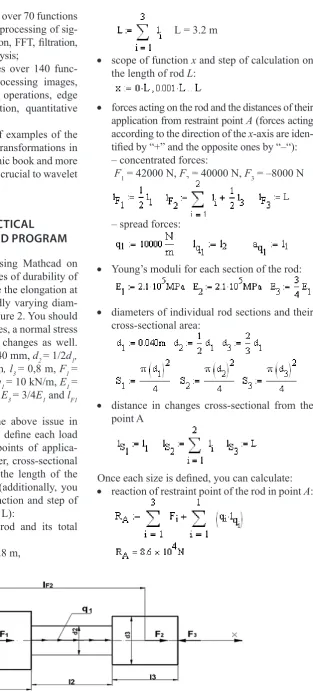
Practical possibilities of using Mathcad on the example of solving the issues of durability of materials. You need to calculate the elongation at break for a steel rod of a rapidly varying diam-eter and loaded as shown in Figure 2. You should construct graphs of normal forces, a normal stress range and cross-sectional area changes as well. Adopt the following data: d₁= 40 mm, d₂= 1/2d₁, d₃= 2/3d₁, l₁= 1,2 m, l₂= 1,2 m, l₃= 0,8 m, F₁= 42 kN, F₂= 40 kN, F₃= 8 kN, q₁= 10 kN/m, E₁= 2,1·105 _MPa,_E

2 = 2,1·105 MPa, E3 = 3/4E1and lF1 = 0,6 m, l_F2= 2,8 m.

Before starting to solve the above issue in Mathcad program, you need to define each load acting on the given rod, the points of applica-tion of these loads, rod diameter, cross-secapplica-tional changes, Young’s moduli and the length of the individual sections of the rod (additionally, you need to define the scope of function and step of calculation on the length of rod L):

• individual sections of the rod and its total length:

l₁ = 1.2 m, l₂ = 1.2 m, l₃ = 0.8 m,

diameter and loaded as shown in fig. 2. You should construct graphs of normal forces, a normal stress range and cross-sectional area changes as well. Adopt the following data: d1=40 mm, d2=1/2d1, d3=2/3d1, l1=1,2 m, l2=1,2 m, l3=0,8 m F1=42 kN, F2=40 kN, F3=8 kN, q1=10 kN/m, E1=2,1·105 _{MPa, E2=2,1·10}5 _{MPa, E3=3/4E1 and lF1=0,6 m, lF2=2,8 m.}

Fig. 2 Scheme of tie rod

Before starting to solve the above issue in Mathcad program, you need to define each load acting on the given rod, the points of application of these loads, rod diameter, cross-sectional changes, Young’s moduli and the length of the individual sections of the rod (additionally, you need to define the scope of function and step of calculation on the length of rod L):

 individual sections of the rod and its total length:

 scope of function x and step of calculation on the length of rod L:

 forces acting on the rod and the distances of their application from restraint point A (forces acting according to the direction of the x-axis are identified by “+” and the opposite ones by “-“):

- concentrated forces:

- spread forces:

L= 3.2 m

• scope of function x and step of calculation on the length of rod L:

- spread forces:

• forces acting on the rod and the distances of their application from restraint point A (forces acting according to the direction of the x-axis are iden-tified by “+” and the opposite ones by “–“): – concentrated forces:

F₁ = 42000 N, F₂ = 40000 N, F₃ = –8000 N

- spread forces:

- spread forces: – spread forces:

- spread forces:

• Young’s moduli for each section of the rod:  Young’s moduli for each section of the rod:

 diameters of individual rod sections and their cross-sectional area:

 distance in changes cross-sectional from the point A

Once each size is defined, you can calculate:

 reaction of restraint point of the rod in point A:

 forces coming from both external concentrated and spread forces acting on the rod:

 normal forces N for each section of the rod:

 cross-sectional areas changing in the range of function X:

 distribution of stresses in the area of function X:

 Young’s moduli for each section of the rod:

 distribution of stresses in the area of function X:  Young’s moduli for each section of the rod:

• diameters of individual rod sections and their cross-sectional area:

• distance in changes cross-sectional from the point A

Once each size is defined, you can calculate: • reaction of restraint point of the rod in point A:

(5)

42

• forces coming from both external concentrated and spread forces acting on the rod:  Young’s moduli for each section of the rod:

• normal forces N for each section of the rod:  Young’s moduli for each section of the rod:

• cross-sectional areas changing in the range of function X:  Young’s moduli for each section of the rod:

 distribution of stresses in the area of function X: • distribution of stresses in the area of function X:  Young’s moduli for each section of the rod:

• Young’s modulus changing in the range of function X:  Young’s modulus changing in the range of function X:

 total elongation:

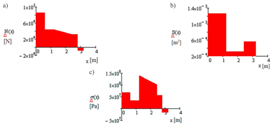
For checking, construct a graph for normal forces, cross-sectional changes, normal stresses occurring in the rod (fig. 3):

a) b)

c)

Fig. 3 Graph of: normal force distribution (a); cross-sectional area changes (b); changes of normal stresses (c) of the rod

As you can see, Mathcad allows you to write computational procedures, or independent programs. They may contain many assigning functions, all kinds of conditional instructions and various options for local and global variables. These programs (procedures) perform calculations automatically. Change in any record makes the whole procedure change. The user can interfere with its record. They can analyse the changes in solving the given issue with different parameters (e.g. variables, values, etc.) on prepared programs. Changes may be presented and analysed in the graphical form. Students, pupils or engineers can use it to solve

• total elongation:

 Young’s modulus changing in the range of function X:

 total elongation:

For checking, construct a graph for normal forces, cross-sectional changes, normal stresses occurring in the rod (fig. 3):

a) b)

c)

Fig. 3 Graph of: normal force distribution (a); cross-sectional area changes (b); changes of normal stresses (c) of the rod

As you can see, Mathcad allows you to write computational procedures, or independent programs. They may contain many assigning functions, all kinds of conditional instructions and various options for local and global variables. These programs (procedures) perform calculations automatically. Change in any record makes the whole procedure change. The user can interfere with its record. They can analyse the changes in solving the given issue with different parameters (e.g. variables, values, etc.) on prepared programs. Changes may be presented and analysed in the graphical form. Students, pupils or engineers can use it to solve

For checking, construct a graph for normal forces, cross-sectional changes, normal stresses occur-ring in the rod (Figure 3).

As it was presented above, Mathcad allows to write computational procedures, or independent pro-grams. They may contain many assigning functions, all kinds of conditional instructions and various options for local and global variables. These programs (procedures) perform calculations automatically.

Fig. 3. Graph of: a – normal force distribution; b – cross-sectional area changes; c – changes of normal stresses of the rod

a) b)

(6)

43

Change in any record makes the whole procedure change. The user can interfere with its record. They can analyse the changes in solving the giv-en issue with differgiv-ent parameters (e.g. variables, values, etc.) on prepared programs. Changes may be presented and analysed in the graphical form. Students, pupils or engineers can use it to solve all kinds of problems in various fields. You can use it to solve more or less advanced issues, be-cause of its fairly extensive computational capa-bilities, which include [11]:

• calculating expressions and functions includ-ing derivatives, integrals and limits,

• solving equations and inequalities,

• solving systems of linear and non-linear equa-tions,

• solving ordinary and partial differential equations,

• performing numerical and symbolic calculations,

• calculations on vectors and matrices,

• finding vectors and eigenvalues of the matrix, • curve fitting to a given system of points on a

surface,

• creating graphs of 2D and 3D functions, • creating three-dimensional animations,

• performing operations on complex numbers,

• built-in probability distribution and statistical functions,

• use of SI, MKS, CGS and US units of measure,

• built-in set of functions (DoE) that reduces time and cost of conducting and analysing ex-periments,

• creating your own subprograms,

• use of upper and lower case letters of the Greek alphabet in expressions,

• comparison of two worksheets,

• data exchange with other programs,

• analysis and synthesis of audio files, • work on bitmaps,

• cooperation with data files, • supporting Unicode,

• additional modules of data analysis, signals, images and wavelet transformations,

• access to the online libraries providing tech-nical information and tools from the fields of engineering,

• transfer of physical quantities and parameter val-ues between the applications in an unified way.

CONCLUSIONS

We can use the computational capabilities of CAS programs in everyday work that requires fre-quent and repeatable use of more or less advanced

mathematical calculations. The opportunities of using Mathcad, which were discussed in this work, can greatly facilitate, improve and accelerate solv-ing different kinds of problems in various fields.

Automation of complex calculations, faced by engineers, helps avoid errors while reducing computation time, which, in turn, translates into the quality and profitability of the project. There -fore, it is very important and advisable to teach CAS programs in vocational and high schools, technical schools and in colleges. They can be used for courses in subjects such as Mathemat -ics, Phys-ics, Electron-ics, Electrical Engineering, Mechanical Engineering, Strength of Materials, Statistics, Computer Aided Engineering Calcu-lations, etc.

REFERENCES

1. Kruczek W.: The electrical characteristics of a cat-enary system in electric rail vehicles, the calcula-tion of traccalcula-tion load and short – circuit currents.

IAPGOŚ 4, 2013, 22–25.

2. Radzieński M., Noga K.: Digital image process

-ing in Mathcad. Scientific Papers of the Faculty of

Electrical and Control Engineering Gdansk Uni-versity of Technology, 25, 2008, 135–139.

3. Hałat W.: Use of computer algebra system for beams‘ bending problems. Mining and Geoengi -neering, 3, 2007, 171–182.

4. Gosowski B., Redecki M.: Solution of torsion problems of continious I-sections using

Mathemat-ica package. Scientific Papers Rzeszów University

of Technology. Construction and Environmental

Engineering, 9(3/II), 2012, 357–364.

5. Galon Z.: Mathcad 13 – application for managing engineering design documents. Electrical Review, 82(6), 2006, 87–88.

6. Noga K.M.: Analog and digital modulations in MATHCAD and VISSIM environment. Scientific

Papers of the Faculty of Electrical and Control En-gineering Gdansk University of Technology, 36, 2013, 137–140.

7. Pashechko M., Bartnicki J., Barszcz M., Kiernicki Z.: Computer-aided in the engineering calculations

– Mathcad. Publisher PWSZ, Zamość 2013.

8. Pashechko M., Barszcz M., Dziedzic K.: The use

Mathcad program to solve of selected engineering issues. Publisher Lublin University of Technology, Lublin 2011.

9. Website: http://www.helionica.pl (Access: Apr. 2014).

10. Motyka R., Rasał D.: MathCAD from the calcula