ACCELERATED METHODS FOR ESTIMATING THE DURABILITY OF PLAIN BEARINGS

73

Research Journal

Volume 8, No. 23, Sept. 2014, pages 73–79

DOI: 10.12913/22998624.1120326 Research Article

Received: 2014.07.19 Accepted: 2014.08.18 Published: 2014.09.09

ACCELERATED METHODS FOR ESTIMATING THE DURABILITY

OF PLAIN BEARINGS

Myron Czerniec1

1 _{Institute of Technological Systems of Information, Lublin University of Technology, Nadbystrzycka 36, 20-612} Lublin, Poland, e-mail: [email protected]

ABSTRACT

The paper presents methods for determining the durability of slide bearings. The de-veloped methods enhance the calculation process by even 100000 times, compared to the accurate solution obtained with the generalized cumulative model of wear. The paper determines the accuracy of results for estimating the durability of bearings de-pending on the size of blocks of constant conditions of contact interaction between the shaft with small out-of-roundedness and the bush with a circular contour. The paper gives an approximate dependence for determining accurate durability using either a more accurate or an additional method.

Keywords: enhanced numerical methods, durability evaluation, plain bearings, ac-curacy deviations.

INTRODUCTION

Plain bearings find numerous applications in machine design as well as in various devices that facilitate human life. The literature on the subject provides simplified methods [1–14] for estimat-ing the durability of these bearestimat-ings where it is as-sumed that the shaft and bush have an ideal (i.e. circular) section of contours. However, in reality these components of slide bearings are produced with out-of-roundness deviations (ovality, trilob-ing, tetralobing) that have – as demonstrated in [15, 16] – an effect on the durability of bearings.

The kinematics of wear of the shaft with out-of-roundedness can be investigated using either the cumulative model of wear [15–17] or the generalized cumulative model of wear [18] for the interval-discrete interaction between bearing components. The cumulative model of wear al-lows estimating the degree of wear and durability of a bearing for single-area contact of the compo-nents, while the generalized cumulative model of wear is applied to examine mixed contact.

The above models entail dividing the contour of the shaft with out-of-roundedness into dis-cretization intervals Δα₂, where both initial

con-tact pressures and concon-tact area are assumed to be constant. In a full rotation of the shaft with out-of-roundedness, there is j-th interaction with the bush (j = 360 °/Δα₂).

Bearing components undergo wear during ro-tation, hence the initial contact parameters change and their wear is cumulative.

With application of the interval-discrete pat-tern of tribocontact interaction, the time of com-putations is considerably long, particularly at low values of the discretization interval Δα₂ of shaft contour that ensure the most accurate numerical solution of the problem. An increase in Δα₂ leads to a proportional decrease in the estimated dura-bility of a bearing. Nonetheless, the computation time still remains considerably long. In order to decrease effectively the time of computations, the express method [19] with an interval-range-block calculation pattern has been developed. The method is based on the assumption that param-eters of contact interaction for particular intervals of discretization remain constant during a certain number of shaft rotations (block size). Such an approach ensures a shorter time of computations, proportionally to the size of a block with con-stant conditions of interaction between the

74

ing components. The present paper presents the results of this problem as solved by the express method using various calculation methods.

CALCULATION

METHODS

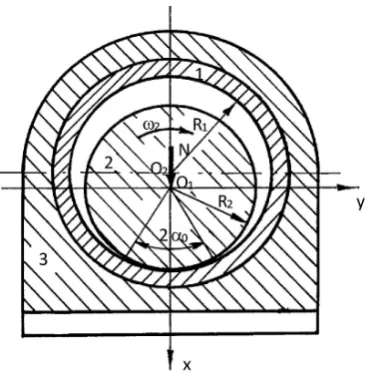
The slide bearing (Fig. 1) carries the load N, while shaft 2 rotates with the angular velocity ω₂. The bearing has a radial clearance of ε = R₁ – R₂, where 2R₁ denotes the nominal diameter of the bush and 2R₂ denotes the diameter of the shaft. Under the action of load, the bearing components contact each other in the 2R₂α₀ area where contact pressures p(α) are generated. The bearing is made of different materials, whose properties and resis-tance to wear differ.

Fig. 1. Schematic diagram of a slide bearing

Due to the fact that the components of bearing exhibit low ovality, they produce either single-ar-ea (Fig. 2a) or double-arsingle-ar-ea (Fig. 2b) contact. Dur-ing a rotation of the shaft (α₂>0), two types of in-teractions are possible: full single-area and mixed (single – double – single-area). The interaction between bearing components with the contour ovality L₁ and L₂ is described by the following contact parameters:

• single area contact (Fig. 2a): 2α_0δ(α₂) – vari-able contact angle, contact pressures p(α₂, δ), maximum contact pressures p(0, δ), contact area W = 2R₂α_0δ;

• mixed contact (Fig. 2b): 2γ – symmetric con-tact angle or asymmetric concon-tact angles 2γ₁(α₂), 2γ₂(α₂); symmetric contact pressures p(γ, δ) and asymmetric contact pressures p(α₂, δ); sym-metric contact area W_1,2 = 2R₂γ and asymmetric contact areas W₁ = 2R₂γ₁, W₂ = 2R₂γ₂.

The contact angle 2λof bearing components is determined by the method discussed in the study [20]. In the case of the symmetric double-area contact (Fig. 2b), the forces N₁ = N₂ = N /(2cosλ).

However, for the asymmetric contact N₁ ≠

N₂, λ₁ ≠ λ₂, 2λ₁ ≠ 2λ₂, p(λ₁, δ) ≠ p(λ₂, δ) [17]. The ovality of contours of the bearing components is described by the deviations δ₁ = R₁ – R₁ʹ, δ₂ = R₂ʹ – R₂ (Fig. 2).

a)

b)

Fig. 2. Single-area (a) and double-area (b) contact of shaft and bush

Using the generalized cumulative model of wear [18], a numerical calculation was performed for the problem of full single-area contact and mixed contact of the bearing components, where the following parameters were applied: N = 0.1 MN;

R₂ = 50 mm; v = 0.0628 m/sec – sliding veloc-ity; f = 0,04 – sliding friction factor at boundary friction; ε = 0.21; 0.41 mm; δ₁ = 0 mm; δ₂ = 0; 0,05; 0,1; 0,15; 0,2; 0,3; 0,4 mm; δ₁ +δ₂ ≤ε; n₂

= 12 rpm – number of rotations of the shaft; h_1* = 0,3 mm – maximum wear of the bush; the shaft

75

is made of steel (hardened + tempered), while the bush is made of bronze CuSn5Zn5Pb5; Δα₂ = 100

– the discretization interval of the shaft contour;

B = 72000, 7200, 720, 12, 1 rotations – block sizes.

RESULTS

The results of solving the problem are listed in:

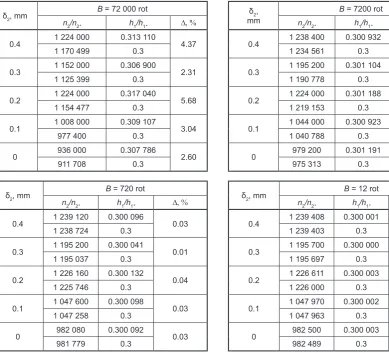
• Tables 1, 2 – the accurate method based on the interval-block pattern (B = 1 rotation);

• Tables 3, 4 (numerator) – the approximate method based on the interval-block pattern (B = 12, 720, 7200, 72 000 rotations);

Table 1. Bearing durability n2* as calculated by the

ac-curate method(ε= 0.21 mm)

δ2, mm

B = 1 rot

n2*,rot h1*, mm

0.2 1 722 413 0.3

0.15 1 663 970 0.3

0.1 1 651 362 0.3

0.05 1 413 160 0.3

0.0 1 332 336 0.3

Table 2. Bearing durability n2*as calculated by the

ac-curate method (ε = 0.41 mm)

δ2, mm

B = 1 rot n2*,rot h1*, mm

0.4 1 239 410 0.3

0.3 1 195 707 0.3

0.2 1 226 752 0.3

0.1 1 047 977 0.3

0 982 501 0.3

Table 3. Bearing durability n_2* calculated by the approximate method (ε = 0.21 mm)

δ2, mm

B = 72 000 rot

n2/n2* h1/h1* D, %

0.2 1 656 000 0.30098 0.33 1 650 535 0.3

0.15 1 656 000 0.31155 3.85 1 592 244 0.3

0.1 1 584 000 0.30110 0.37 1 578 139 0.3

0.05 1 368 000 0.30570 1.9 1 342 008 0.3

0 1 296 000 0.31040 3.47 1 251 029 0.3

δ2, mm

B = 7200 rot

n2/n2* h1/h1* D, %

0.2 1 720 800 0.30098 0.33 1 715 121 0.3

0.15 1 663 200 0.30116 0.39 1 691 205 0.3

0.1 1 648 800 0.30110 0.37 1 642 700 0.3

0.05 1 411 200 0.30110 0.37 1 405 979 0.3

0 1 324 800 0.30048 0.16 1 322 680 0.3

δ2, mm

B = 720 rot

n2/n2* h1/h1* D, %

0.2 1 722 240 0.3001 0.03 1 721 723 0.3

0.15 1 663 920 0.30012 0.04 1 663 255 0.3

0.1 1 650 960 0.3001 0.03 1 650 415 0.3

0.05 1 412 410 0.3000 0.00 1 412 410 0.3

0 1 332 000 0.3001 0.03 1 331 560 0.3

δ2, mm

B = 12 rot

n2/n2* h1/h1* D, %

0.2 1 722 396 0.3000 0.00 1 722 396 0.3

0.15 1 663 944 0.3000 0.00 1 663 944 0.3

0.1 1 651 348 0.3000 0.00 1 651 348 0.3

0.05 1 413 156 0.3000 0.00 1 413 156 0.3

0 1 332 320 0.3000 0.00 • Tables 3, 4 (denominator) – the more accurate

method based on the results of the approxi-mate solution.

An increase in radial clearance leads to de-creased durability of the bearing.

Here, the actual wear h₁ of the bush is always somewhat higher than the maximum wear h_1*

(Tables 3, 4).

The bearing durability h_1* was estimated more accurately based on its approximate durability n₂

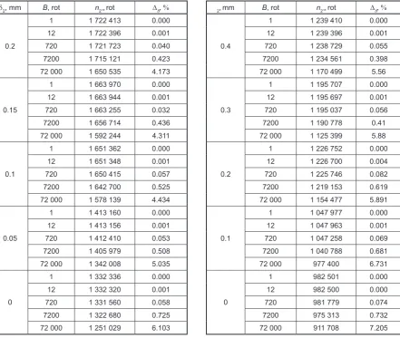
and the corresponding wear h₁ > h_1* of the bushin the following way: n_2* = n₂(h_1*/h₁). Tables 5 and 6 give the deviations Δ_B of the solutions.

76

The analysis of the obtained results dem-onstrates that an increase in block size leads to higher deviations Δ_B. At radial clearance ε = 0.21 mm (Table 5), for B = 720 rotations, the estimated durability decreases by 0.04–0.058% compared to the accurate durability (B = 1 rot); for B = 7200 rotations it decreases by 0.42–0.730%; for

B = 72000 rotations it decreases by 4.17–6.1% depending on shaft ovality value. In the case of shafts with a circular section (δ₂ = 0), the de-viations will be the highest. If radial clearances increase, the deviation Δ_B increases as well, as shown in Table 6 for ε = 0.41 mm. It is assumed that block В = 7200 rotations will be optimum for the discretization interval Δα₂ = 100 _;

Table 7 list an additive method based on the adjusted interval-block pattern (В = 72000 → 7200 → 720 → 12 → 1 rot), using the formula:

8

% depending on shaft ovality value. In the case of shafts with a circular section

(2= 0), the deviations will be the highest. If radial clearances increase, the

deviation ΔB increases, too, as shown in Table 6 for ε= 0.41 mm. It is assumed

that block В = 7200 rotations will be optimum for the discretization interval

2



 = 100 _;

d) the additive method based on the adjusted interval – block pattern (В =

72000  7200  720  12  1 rot) (Table 7)

n2*x B1 72000x B2 7200x B3 720x B4 12x B5 1, (1)

where x1 is the maximum number of basic blocks Bp, for which h1h1*;

x2, x3, x4 are the respectively maximum number of successive block sizes

which will satisfy a given condition;

x5 is the number of blocks B = 1 rotation that ensure obtaining the accurate

value of wear h1*.

Table 7. Bearing durability for different sizes of basic blocks (ε= 0.41 mm)

2

δ , mm B = 1 rot Вp = 7200 rot Вp = 72000 rot

2*

n , rot n2*, rot ΔΣ,% n2*, rot ΔΣ,%

0.4 1239410 1232469 0.56 1170375 5.57

0.3 1195707 1189011 0.56 1125160 5.90 0.2 1226752 1219141 0.62 1154341 5.90

0.1 1047977 1040733 0.69 975973 6.87

0 982501 975301 0.73 910501 7.33

Note: ΔΣ – deviations of the additive durability from the accurate durability (B

= 1 rotation)

The results of investigating the effect of size of blocks of constant conditions of contact on the durability of a bearing with shaft ovality demonstrate that the deviations from the accurate result caused by blocks with a size of up to 10000

rotations do not exceed 1 % , which is also the number of times by which the

computation time is reduced.

For practical reasons, the additive method based on the adjusted interval –

block pattern is most rational to apply to solve the problem. Apart from a much simpler and faster procedure of numerical calculation, the accuracy of results obtained is similar to the results obtained with the more accurate method (Tables 5, 6). Analyzing the durability estimation results (Tables 5÷7), it is found that

the durability ( )

2D

n of the accurate solution can be determined based on the

durability ( )

2Dk n or ( )

2A

n in the following way:

(1) where: x₁ is the maximum number of basic blocks

B_p, for which h₁ < h_1*;

x₂, x₃, x₄ are the respectively maximum number of successive block sizes which

Table 4. Bearing durability n_2*calculated by the approximate method (ε = 0.41 mm)

δ2, mm

B = 72 000 rot

n2/n2* h1/h1* D, %

0.4 1 224 000 0.313 110 4.37 1 170 499 0.3

0.3 1 152 000 0.306 900 2.31 1 125 399 0.3

0.2 1 224 000 0.317 040 5.68 1 154 477 0.3

0.1 1 008 000 0.309 107 3.04 977 400 0.3

0 936 000 0.307 786 2.60 911 708 0.3

δ2, mm

B = 720 rot

n2/n2* h1/h1* D, %

0.4 1 239 120 0.300 096 0.03 1 238 724 0.3

0.3 1 195 200 0.300 041 0.01 1 195 037 0.3

0.2 1 226 160 0.300 132 0.04 1 225 746 0.3

0.1 1 047 600 0.300 098 0.03 1 047 258 0.3

0 982 080 0.300 092 0.03 981 779 0.3

δ2, mm

B = 7200 rot

n2/n2* h1/h1* D, %

0.4 1 238 400 0.300 932 0.31 1 234 561 0.3

0.3 1 195 200 0.301 104 0.37 1 190 778 0.3

0.2 1 224 000 0.301 188 0.40 1 219 153 0.3

0.1 1 044 000 0.300 923 0.31 1 040 788 0.3

0 979 200 0.301 191 0.40 975 313 0.3

δ2, mm

B = 12 rot

n2/n2* h1/h1* D, %

0.4 1 239 408 0.300 001 0.00 1 239 403 0.3

0.3 1 195 700 0.300 000 0.00 1 195 697 0.3

0.2 1 226 611 0.300 003 0.00 1 226 000 0.3

0.1 1 047 970 0.300 002 0.00 1 047 963 0.3

0 982 500 0.300 003 0.00 982 489 0.3

will satisfy a given condition;

x₅ is the number of blocks B = 1 rotation that ensure obtaining accurate value of wear h_1*.

The results of investigating the effect of the size of blocks of constant conditions of contact on the durability of a bearing with shaft ovality demonstrate that the deviations from the accu-rate result caused by blocks with a size of up to 10000 rotations do not exceed 1%, which is also the number of times by which the computation time is reduced.

For practical reasons, the additive method based on the adjusted interval – block pattern is most rational to apply to solve the problem. Apart from a much simpler and faster procedure of numerical calculation, the accuracy of results obtained is similar to the results obtained with a more accurate method (Tables 5, 6). Analyzing the durability estimation results (Tables 5–7), it is found that the durability n_2*(D)_{of the accurate}

solution can be determined based on the durabil-ity n_2*(Dk) _{or n}

2*(A) in the following way:

77

Table 5. Deviations of the approximate durability with

regard to the accurate one (ε = 0.21 mm) Table 6. regard to the accurate one (Deviations of the approximate durability with ε = 0.41 mm).

9

( ) ( ) 2D  2Dk 

n n B lub ( ) ( )

2D  2A  p

n n B , (2)

where (Dk) and (A) denote, respectively, the more accurate and additive methods

for solving the problem.

Tables 8 and 9 list durability differences ( ) ( ) ( )

2 2 2 2

Δn nD nDk,nA which

confirm the formula (2).

Table 8. Differences Δn₂n₂( )D n( )₂Afor the durability D and Dk (ε= 0.41 mm)

2

δ , mm _{B, rot} n_2*, rot Δn₂rot

0.4

1 1239410 -

12 1239396 14

720 1238729 681

7200 1234561 4849

72000 1170499 68911

0.3

1 1195707 -

12 1195697 10

720 1195037 670

7200 1190778 4929

72000 1125399 70308

0.2

1 1226752 -

12 1226700 52

720 1225746 1006

7200 1219153 7599

72000 1154477 72275

0.1

1 1047977 -

12 1047963 14

720 1047258 719

7200 1040788 7189

72000 977400 70577

0

1 982501 -

12 982500 1

720 981779 722

7200 975313 7188

72000 911708 70793

Table 9. Differences Δn2n( )2D n( )2A for the durability D and A (ε= 0.41 mm)

2

δ , mm B = 1 rot Вp = 7200 rot Вp = 72000 rot

2*

n , rot n2*, rot Δn2rot n2*, rot Δn2rot

0.4 1239410 1232469 6941 1170375 69035

0.3 1195707 1189011 6696 1125160 70547

0.2 1226752 1219141 7611 1154341 72411

0.1 1047977 1040733 7244 975973 72004

0 982501 975301 7200 910501 72000

or

9

( ) ( ) 2D  2Dk 

n n B lub ( ) ( )

2D  2A  p

n n B , (2)

where (Dk) and (A) denote, respectively, the more accurate and additive methods

for solving the problem.

Tables 8 and 9 list durability differences ( ) ( ) ( )

2 2 2 2

Δn nD nDk,nA which

confirm the formula (2).

Table 8. Differences Δn₂n₂( )D n( )₂Afor the durability D and Dk (ε= 0.41 mm)

2

δ , mm _{B, rot} n_2*, rot Δn₂rot

0.4

1 1239410 -

12 1239396 14

720 1238729 681

7200 1234561 4849

72000 1170499 68911

0.3

1 1195707 -

12 1195697 10

720 1195037 670

7200 1190778 4929

72000 1125399 70308

0.2

1 1226752 -

12 1226700 52

720 1225746 1006

7200 1219153 7599

72000 1154477 72275

0.1

1 1047977 -

12 1047963 14

720 1047258 719

7200 1040788 7189

72000 977400 70577

0

1 982501 -

12 982500 1

720 981779 722

7200 975313 7188

72000 911708 70793

Table 9. Differences Δn2n( )2D n2( )A for the durability D and A (ε= 0.41 mm)

2

δ , mm B = 1 rot Вp = 7200 rot Вp = 72000 rot

2*

n , rot n2*, rot Δn2rot n2*, rot Δn2rot

0.4 1239410 1232469 6941 1170375 69035

0.3 1195707 1189011 6696 1125160 70547

0.2 1226752 1219141 7611 1154341 72411

0.1 1047977 1040733 7244 975973 72004

0 982501 975301 7200 910501 72000

(2) where: (Dk) and (A) denote, respectively, the

more accurate and additive methods for solving the problem.

Tables 8 and 9 list durability differences 9

( ) ( ) 2D  2Dk 

n n B lub ( ) ( )

2D  2A  p

n n B , (2)

where (Dk) and (A) denote, respectively, the more accurate and additive methods

for solving the problem.

Tables 8 and 9 list durability differences ( ) ( ) ( )

2 2 2 2

Δn nD nDk,nA which

confirm the formula (2).

Table 8. Differences Δn₂n₂( )D n( )₂Afor the durability D and Dk (ε= 0.41 mm)

2

δ , mm _{B, rot} n_2*, rot Δn₂rot

0.4

1 1239410 -

12 1239396 14

720 1238729 681

7200 1234561 4849

72000 1170499 68911

0.3

1 1195707 -

12 1195697 10

720 1195037 670

7200 1190778 4929

72000 1125399 70308

0.2

1 1226752 -

12 1226700 52

720 1225746 1006

7200 1219153 7599

72000 1154477 72275

0.1

1 1047977 -

12 1047963 14

720 1047258 719

7200 1040788 7189

72000 977400 70577

0

1 982501 -

12 982500 1

720 981779 722

7200 975313 7188

72000 911708 70793

Table 9. Differences Δn2n2( )D n( )2Afor the durability D and A (ε= 0.41 mm)

2

δ , mm B = 1 rot Вp = 7200 rot Вp = 72000 rot

2*

n , rot n2*, rot Δn2rot n2*, rot Δn2rot

0.4 1239410 1232469 6941 1170375 69035

0.3 1195707 1189011 6696 1125160 70547

0.2 1226752 1219141 7611 1154341 72411

0.1 1047977 1040733 7244 975973 72004

0 982501 975301 7200 910501 72000

which confirm the for-mula (2).

d₂, mm B, rot n2*,rot DB, %

0.2

1 1 722 413 0.000 12 1 722 396 0.001 720 1 721 723 0.040 7200 1 715 121 0.423 72 000 1 650 535 4.173

0.15

1 1 663 970 0.000 12 1 663 944 0.001 720 1 663 255 0.032 7200 1 656 714 0.436 72 000 1 592 244 4.311

0.1

1 1 651 362 0.000 12 1 651 348 0.001 720 1 650 415 0.057 7200 1 642 700 0.525 72 000 1 578 139 4.434

0.05

1 1 413 160 0.000 12 1 413 156 0.001 720 1 412 410 0.053 7200 1 405 979 0.508 72 000 1 342 008 5.035

0

1 1 332 336 0.000 12 1 332 320 0.001 720 1 331 560 0.058 7200 1 322 680 0.725 72 000 1 251 029 6.103

2,mm B, rot n2*,rot DB, %

0.4

1 1 239 410 0.000 12 1 239 396 0.001 720 1 238 729 0.055 7200 1 234 561 0.398 72 000 1 170 499 5.56

0.3

1 1 195 707 0.000 12 1 195 697 0.001 720 1 195 037 0.056 7200 1 190 778 0.41 72 000 1 125 399 5.88

0.2

1 1 226 752 0.000 12 1 226 700 0.004 720 1 225 746 0.082 7200 1 219 153 0.619 72 000 1 154 477 5.891

0.1

1 1 047 977 0.000 12 1 047 963 0.001 720 1 047 258 0.069 7200 1 040 788 0.681 72 000 977 400 6.731

0

1 982 501 0.000 12 982 500 0.000 720 981 779 0.074 7200 975 313 0.732 72 000 911 708 7.205

Table 7. Bearing durability for different sizes of basic blocks (ε = 0.41 mm)

d₂, mm B = 1 rot Вp = 7200 rot Вp = 72 000 rot

n2*, rot n2*, rot D Σ,% n2*, rot D Σ, %

0.4 1 239 410 1 232 469 0.56 1 170 375 5.57

0.3 1 195 707 1 189 011 0.56 1 125 160 5.90

0.2 1 226 752 1 219 141 0.62 1 154 341 5.90

0.1 1 047 977 1 040 733 0.69 975 973 6.87

0 982 501 975 301 0.73 910 501 7.33

Note: D Σ – deviations of the additive durability from the accurate durability (B = 1 rotation).

CONCLUSIONS

1. Values of deviations of durability determined by the more accurate and additive methods were compared to those obtained by the ac-curate method.

2. It is found that the computation time decreas-es directly proportional to the size of blocks of constant conditions of interaction.

Advances in Science and Technology Research Journal vol. 8 (23) 2014

78

3. We have got an approximate dependence for estimating accurate durability of a bear-ing based on the more accurate and additive method.

4. It is found that the additive method is a simple and effective way of solving the problem of estimating the durability of a slide bearing.

REFERENCES

1. Andrejkiv A.E., Czerniec M.V.: Ocenka kontaktno-go vzaimodiejstvija truszczichsia dietaliej maszyn. Naukova Dumka, Kijev, 1991.

2. Goriaczeva I.G., Dobyczin N.M.: Kontaktnyje zadaczi v tribologii. Maszinostrojenije, Moskva, 1988.

3. Kovalenko E.V.: K rasczetu iznaszivanija

soprjażenija vał – vtułka. Mechanika Tverdoho Tieła, 6, 1982, 66–72.

4. Kuźmenko A.G.: Metody rozrachunkiv na znoszu-vannja ta nadijnist. TUP, Chmelnyckyj, 2002.

5. Kragielskij I.V., Dobyczin N.M., Kombalov V.S.: Osnovy rasczetov na trenie i iznos. Maszinostroenie, 1977, pp. 526.

6. Tepłyj M.I.: Opredielienije kontaktnych

parami-etrov i iznosa v cilindriczeskich oporach skolżenija. Trenije i Iznos, 6, 1987, 895–902.

7. Tepłyj M.I.: Kontaktnyje zadaczi dla oblastej s

kruhowymi granicami. Lwow, Wyszcza Szkoła, Wyd. LGU, 1983, pp. 176.

8. Usov P.P.: Vnutrennij kontakt cilindriczeskich tieł

blizkich radiusov pri iznaszivanii ich

poverch-nostiej. Trenije i Iznos, 3, 1985, 404–414.

9. Zwierzycki W.: Prognozowanie niezawodności zużywających się elementów maszyn. Radom,

Wyd. ITE, 1998.

10. Sorokatyj R.V.: Uzahalnennia metodu trybo-elementiv dla modeljuvannia procesiv znoszu-vannia v pidszypnykach kovzannia. Problemy Try-bologii, 2, 2007, 36–45.

11. Sorokatyj R.V.: Reszenije iznosokontaktnych za-dacz metodom triboelementov v sredie konieczno-elementnogo pakieta ANSYS. Problemy Trybolo-gii, 3, 2007, 9–17.

12. Kolmogorov V.L., Kharlamov V.V., Kurilov A.M., Pavlishko S.V.: Friction and wear model for a heav-ily loaded sliding pair. Part II. Application to an

un-lubricated journal bearing. Wear, 197, 1996, 9–16. Table 8. Differences

( ) ( ) 2D  2Dk 

n n B lub ( ) ( )

2D  2A  p

n n B , (2) where (Dk) and (A) denote, respectively, the more accurate and additive methods for solving the problem.

Tables 8 and 9 list durability differences ( ) ( ) ( )

2 2 2 2

Δn nD nDk ,nA which confirm the formula (2).

Table 8. Differences Δn2n( )2D n( )2Afor the durability D and Dk (ε= 0.41 mm)

2

δ , mm _{B, rot} n2*, rot Δn2rot

0.4

1 1239410 -

12 1239396 14

720 1238729 681

7200 1234561 4849

72000 1170499 68911

0.3

1 1195707 -

12 1195697 10

720 1195037 670

7200 1190778 4929

72000 1125399 70308

0.2

1 1226752 -

12 1226700 52

720 1225746 1006

7200 1219153 7599

72000 1154477 72275

0.1

1 1047977 -

12 1047963 14

720 1047258 719

7200 1040788 7189

72000 977400 70577

0

1 982501 -

12 982500 1

720 981779 722

7200 975313 7188

72000 911708 70793

Table 9. Differences Δn2n2( )D n2( )Afor the durability D and A (ε= 0.41 mm)

2

δ , mm B = 1 rot Вp = 7200 rot Вp = 72000 rot

2*

n , rot n2*, rot Δn2rot n2*, rot Δn2rot

0.4 1239410 1232469 6941 1170375 69035

0.3 1195707 1189011 6696 1125160 70547

0.2 1226752 1219141 7611 1154341 72411

0.1 1047977 1040733 7244 975973 72004

0 982501 975301 7200 910501 72000

( ) ( ) 2D  2Dk 

n n B lub ( ) ( )

2D  2A  p

n n B , (2) where (Dk) and (A) denote, respectively, the more accurate and additive methods for solving the problem.

Tables 8 and 9 list durability differences ( ) ( ) ( )

2 2 2 2

Δn nD nDk ,nA which

confirm the formula (2).

Table 8. Differences Δn2n2( )D n2( )Afor the durability D and Dk (ε= 0.41 mm)

2

δ , mm _{B, rot} n2*, rot Δn2rot

0.4

1 1239410 -

12 1239396 14

720 1238729 681

7200 1234561 4849

72000 1170499 68911

0.3

1 1195707 -

12 1195697 10

720 1195037 670

7200 1190778 4929

72000 1125399 70308

0.2

1 1226752 -

12 1226700 52

720 1225746 1006

7200 1219153 7599

72000 1154477 72275

0.1

1 1047977 -

12 1047963 14

720 1047258 719

7200 1040788 7189

72000 977400 70577

0

1 982501 -

12 982500 1

720 981779 722

7200 975313 7188

72000 911708 70793

Table 9. Differences Δn2n( )2D n( )2Afor the durability D and A (ε= 0.41 mm)

2

δ , mm B = 1 rot Вp = 7200 rot Вp = 72000 rot

2*

n , rot n2*, rot Δn2rot n2*, rot Δn2rot

0.4 1239410 1232469 6941 1170375 69035

0.3 1195707 1189011 6696 1125160 70547

0.2 1226752 1219141 7611 1154341 72411

0.1 1047977 1040733 7244 975973 72004

0 982501 975301 7200 910501 72000

for the durabil-ity D and Dk (ε = 0.41 mm)

d₂, mm B, rot n2*, rot Dn2, rot

0.4

1 1 239 410 – 12 1 239 396 14 720 1 238 729 681 7200 1 234 561 4849 72 000 1 170 499 68 911

0.3

1 1 195 707 – 12 1 195 697 10 720 1 195 037 670 7200 1 190 778 4929 72 000 1 125 399 70 308

0.2

1 1 226 752 – 12 1 226 700 52 720 1 225 746 1006 7200 1 219 153 7599 72 000 1 154 477 72 275

0.1

1 1 047 977 – 12 1 047 963 14 720 1 047 258 719 7200 1 040 788 7189 72 000 977 400 70 577

0

1 982 501 –

12 982 500 1

720 981 779 722 7200 975 313 7188 72 000 911 708 70 793

Table 9.Differences

9

( ) ( ) 2D  2Dk 

n n B lub ( ) ( )

2D  2A  p

n n B , (2) where (Dk) and (A) denote, respectively, the more accurate and additive methods for solving the problem.

Tables 8 and 9 list durability differences ( ) ( ) ( )

2 2 2 2

Δn nD nDk,nA which

confirm the formula (2).

Table 8. Differences Δn2n( )2D n( )2Afor the durability D and Dk (ε= 0.41 mm)

2

δ , mm _{B, rot} n2*, rot Δn2rot

0.4

1 1239410 -

12 1239396 14

720 1238729 681

7200 1234561 4849

72000 1170499 68911

0.3

1 1195707 -

12 1195697 10

720 1195037 670

7200 1190778 4929

72000 1125399 70308

0.2

1 1226752 -

12 1226700 52

720 1225746 1006

7200 1219153 7599

72000 1154477 72275

0.1

1 1047977 -

12 1047963 14

720 1047258 719

7200 1040788 7189

72000 977400 70577

0

1 982501 -

12 982500 1

720 981779 722

7200 975313 7188

72000 911708 70793

Table 9. Differences Δn2n( )2D n2( )Afor the durability D and A (ε= 0.41 mm)

2

δ , mm B = 1 rot Вp = 7200 rot Вp = 72000 rot

2*

n , rot n2*, rot Δn2rot n2*, rot Δn2rot

0.4 1239410 1232469 6941 1170375 69035

0.3 1195707 1189011 6696 1125160 70547

0.2 1226752 1219141 7611 1154341 72411

0.1 1047977 1040733 7244 975973 72004

0 982501 975301 7200 910501 72000 9

( ) ( ) 2D  2Dk 

n n B lub ( ) ( )

2D  2A  p

n n B , (2) where (Dk) and (A) denote, respectively, the more accurate and additive methods for solving the problem.

Tables 8 and 9 list durability differences ( ) ( ) ( )

2 2 2 2

Δn nD nDk ,nA which

confirm the formula (2).

Table 8. Differences Δn2n2( )D n2( )Afor the durability D and Dk (ε= 0.41 mm)

2

δ , mm _{B, rot} n2*, rot Δn2rot

0.4

1 1239410 -

12 1239396 14

720 1238729 681

7200 1234561 4849

72000 1170499 68911

0.3

1 1195707 -

12 1195697 10

720 1195037 670

7200 1190778 4929

72000 1125399 70308

0.2

1 1226752 -

12 1226700 52

720 1225746 1006

7200 1219153 7599

72000 1154477 72275

0.1

1 1047977 -

12 1047963 14

720 1047258 719

7200 1040788 7189

72000 977400 70577

0

1 982501 -

12 982500 1

720 981779 722

7200 975313 7188

72000 911708 70793

Table 9. Differences Δn2n2( )D n( )2Afor the durability D and A (ε= 0.41 mm)

2

δ , mm B = 1 rot Вp = 7200 rot Вp = 72000 rot

2*

n , rot n2*, rot Δn2rot n2*, rot Δn2rot

0.4 1239410 1232469 6941 1170375 69035

0.3 1195707 1189011 6696 1125160 70547

0.2 1226752 1219141 7611 1154341 72411

0.1 1047977 1040733 7244 975973 72004

0 982501 975301 7200 910501 72000

for the durability D and A (ε = 0.41 mm)

d₂, mm B = 1 rot Вp = 7200 rot Вp = 72 000 rot

n2*, rot n2*, rot Dn2, rot n2*, rot Dn2, rot

0.4 1 239 410 1 232 469 6941 1 170 375 69 035

0.3 1 195 707 1 189 011 6696 1 125 160 70 547

0.2 1 226 752 1 219 141 7611 1 154 341 72 411

0.1 1 047 977 1 040 733 7244 975 973 72 004

0 982 501 975 301 7200 910 501 72 000

79

13. Rezaei A., Ost W., Paepegem W.V., Degrieck J., Debaets P.: Experimental study and numerical sim-ulation of the large-scale testing of polymeric com-posite journal bearings: two-dimensional modeling

and validation. Wear, 270, 2011, 431–438.

14. Rezaei A., Paepegem W. V., Debaets P., Ost W., Degrieck J.: Adaptive finite element simulation

of wear evolution in radial sliding bearings. Wear,

296, 2012. 660–671.

15. Czerniec M.V., Liebiedieva N.M.: Ocinka kinetyky znoszuvannia trybosystem kovzannia pry najavnosti ovalnosti konturiv ich elementiv za kumuliacijnoju modellu. Problemy Trybologii, 4,

2005, 114–120.

16. Chernets M.V., Andreikiv O.E., Liebiedieva N.M., Zhydyk V.B.: A model for evaluation of wear and durability of plain bearing with small non-circu-larity of its contours. Materials Science, 2, 2009, 279–290.

17. Czerniec M., Żydyk W., Czerniec J.: Symulacja zużywania łożyska ślizgowego z niekołowością

konturów. Cz. 1. Uogólniony model liniowy

zużywania. W: Projektowanie i sterowanie pro -cesami. Lublin, Wyd. Politechniki Lubelskiej,

2013, 76–89.

18. Czerniec M., Żydyk W., Czerniec J.: Symulacja

zużywania łożyska ślizgowego z niekołowością konturów. Cz. 2. Uogólniony model kumulacyjny zużywania. W ks.: Projektowanie i sterowanie pro -cesami. Lublin, Wyd. Politechniki Lubelskiej, 2013,

90–104.

19. Czerniec M.V.: Addytyvnyj metod ocinky dovhovicznosti pidszypnyka kovzannia. Problemy Trybologii, 4, 2013, 20–24.

20. Chernets M.V.: A Contact Problem for a Cylin-drical joint with Technological Faceting of the

Contours of its Parts. Materials Science, 6, 2009, 859–868.