State Space Modelling Using Particle Filtering

(1)

State Space Modelling Using Particle Filtering

G. Ravi Shankar

Aditya Institute of Technology and Management, Srikakulam, Andhra Pradesh, India

A. S. Srinivasa Rao

Aditya Institute of Technology and Management, Srikakulam, Andhra Pradesh, India

Abstract – In any signal/image/video/process engineering state modelling takes leading role. In state modelling, On-line state estimation is a key element. When state functions are highly non-linear and the posterior probability of the state is non-Gaussian, then any one of the conventional filter could not provide efficient and satisfactory results. It is typically crucial to process data online as it arrives, it is both from the point of view of storage cost as well as for rapid adaptation to changing signal characteristics. This paper proposes an alternative approach of conventional filtering techniques is particle filtering. We reviewed Bayesian algorithm for non-linear and non-Gaussian tracking problems with a focus on particle filtering.

Particle filters are working based on the

SEQUENTIAL MONTE-CARLO METHOD’s.

Sequential* Monte-Carlo method based on point mass representations of probability densities, which can be mostly applying to state space modelling and generalises the traditional Kalman filtering methods. Particle filtering is described prior to discussing a number of implementation issues used for the estimation task. Furthermore, MARKOV CHAIN MONTE-CARLO METHOD is proposed to enhance particle filters where the estimation of the initial conditions is poor. The effectiveness of particle filtering of state estimation is explained.

Keywords – On-Line State Estimation, State Space Modelling, Kalman Filtering, Extended Kalman Filtering, Particle Filtering, Markov Chain Monte-Carlo Method (Sequential).

I. I

NTRODUCTION

Most of the applications, it is necessary to estimate the state of the system for calculating the any disturbances (noise, fluctuations, distortions, information loss etc.,). By calculating the states of the system with respective to individual time periods, we may estimate the loss of a signal. Whenever the system is linear and Gaussian then the efficient state estimation can be done using most of the classical filters, like Kalman filters, extended Kalman filters, and unscented Kalman filters. Kalman filters are the perfect and most efficient filters for linear systems only. Whenever the system is non-linear then Kalman filter will not be able to perform the efficient estimation. It might be the basic disadvantage of the Kalman filters. For getting remedy of the Kalman filters, we may use extended Kalman filters. By using extended Kalman filters we may find the efficient estimations for non-linear

systems. But when the system is suffering with Gaussianity then only it will works. While coming for the non-gaussianity it will not estimate the state efficiently. Hence, it is also to all the applications of classical filters. As a remedy of the both Kalman filter and extended Kalman filters there is one more classical filter named as unscented Kalman filter. Which is classical filter mostly works for state estimation of the non-linear systems having non-Gaussianity feature. By using this unscented Kalman filtering, most of the applications may executed or estimated while coming for the estimation of the states, it held efficiently in stable and stored information only. Means it will not give the efficient estimation of states for online estimation (will not be able to operate/ calculate efficient state estimation). We may consider this as a drawback because of now-a-days time and storage are the basic considerations. If we are capable to do in online then there is no need of storage and most of the time going to be save. Hence, then as a remedy of all these problems one non-classical filter is invented which is named as particle filter.

Now-a-days most of the systems having elements of non-linearity and non-gaussianity. These two are having analytical computations. Due to this any of the classical filters will not be able to provide the best state estimations. But one of the non-classical filters named particle filter. In this approach of particle filtering basically two types of approaches. They are Importance sampling and Importance Re-sampling. These are only useful for efficient state estimations. These state estimations can be done by using two procedures named as Prediction and Updation. Prediction is nothing but default value of state for calculating estimation of next state. While completing the calculation of states, the resultant estimated state is known as updated estimated state. In chapter (ii) we are discussed about the kalman filter. In chapter (iii), we have to discussed about the update version of the kalman filter that is extended kalman filter. In chapter (iv), here we discussed about the particle filtering technique.

II. K

ALMAN

F

ILTER

R.E. Kalman has been published and describes a solution to the recursive of discrete data linear filtering problem at 1960[1]. Kalman filter is also known as the “linear quadratic estimation (LQE)”.Kalman filter is not only works well in practice, but also the theoretically attractive because it can be shown that of all possible filters, it is the one that minimizes the variance of the estimation error.

(2)

from a series of noisy measurements. Together with linear quadratic regulator, the Kalman filter solves the linear quadratic Gaussian control problem (LQG)[2]. Kalman filter, LQR and LQG are the solutions of most fundamental problems in control theory.

In simple case, various matrices are constant with time, and thus the subscripts are dropped. But the Kalman filter allows any of them to change each time step[3]. The Kalman filter model assumes the true state at time is evolved from the state at( − 1).

= + + (1)

Where

is the state transition model which applies to the previous state ;

is the control input model which is applied to the control vector ;

Wkis the process noise which is assumed to be drawn

from a zero mean multi-vibrate normal distribution with covariance .

~ (0, )

is real valued Gaussian variable

At time K on observation of the true state is made according to

= + (2)

Where Observation model which maps the true state space into the observed space.

Observation noise which is assumed to be zero means Gaussian white noise with co-variance .

∼ (0, )

The initial state, the noise vectors at each step { , , . . . , . . . }are all assumed to be mutually independent.

Kalman filter can be written in a single equation. But it most often conceptualized as two distinct phases. They are Predict and Update. In predict phase uses the state estimate from the previous time step to produce an estimate of the state at the current time step. Predicted state estimate is also known as the priori state estimate. Because, although it is an estimate of the state at the current time step. In update phase, the current a priori prediction is combined with current observation information to refine the state estimate. Update state is also known as a posterior state estimate. To determine the estimate of the state ‘x’ an estimator is required. The estimator satisfies the two requirements, The average value of state estimate to be equal to average value of the true state. Mathematically, the expected value of the estimate should be equal to the expected value of the state. A state estimate that varies from the true state as little as possible. That is, not only the average of the state estimate to be equal to average of the true state, but also an estimator is required which results in the smallest possible variation of the state estimate. Mathematically an estimator is required with the smallest possible error variances.

III. E

XTENDED

K

ALMAN

F

ILTER

In estimation theory, the extended Kalman filter is the non linear version of the Kalman filter which linearized

about an estimate of the current mean and covariance. Best ever solution for non linear filtering for nonlinear systems estimation. the most widely used estimator for nonlinear filtering is extended kalman filter. Primary drawback of

Kalman filter is that it is optimal estimate for linear system

models with additive independent white noise in both transition and measurement systems. But most of systems are nonlinear. For these non linear systems we will go for the extended Kalman filter. If the system model is not well known, then Monte - Carlo methods, especially particle filters are employed for estimation. While in the use of extended kalman filter there are two drawbacks[4]. 1. Linearization can produce highly unstable filters if the

assumptions of local linearly are violated.

2. The derivation of the Jacobian matrices is Non trivial in most application and often lead to significant implementation difficulties.

The extended kalman filter solves the problem by calculating the jacobian of f and h around the estimated state. In the extended Kalman filter, the state transition and observation models need not be linear functions of the state but may instead be differentiable functions.

= ( , ) + (3)

= ℎ( ) + (4)

, are the process and observation noises are both assumed to be zero mean multi-vibrate Gaussian noises with covariance and respectively. Function ‘f’ can be used to compute the predicted state from the previous estimate. Function ‘h’ can be used to compute the predicted measurement from the predicted state. However f and h cannot be applied to the covariance directly. At each time step, the Jacobean is evaluated with current predicted states. These matrices can be used in the Kalman filter equations. This process essentially linearized the non linear function around the current estimate.

Whenever the initial state estimation is going to be wrong, the filter may quickly diverge from the linearization of the non-linearity. Another problem with the extended Kalman filter is that the estimated covariance matrices tends to underestimate the true covariance matrices and therefore risks becoming inconsistence without the addition of stabilizing noise.

IV. P

ARTICLE

F

ILTER

In statistics, particle filter is also known as a sequential Monte-Carlo method [5]. It is a model estimation technique based on simulation. These are used to estimate Bayesian models in which latent variables are connected in a Markov chain, which is similar to hidden Markov models. But typically where the state space of the latent variables is continuous rather than discrete. Particle filters are so named because they allow for approximate filtering using a set of particles. Particle filters are the sequential analogue of Markov chain Monte Carlo batch methods which are often similar to importance sampling methods. These are much faster than MCMC. These are often an alternative to the EKF or UKF.

(3)

all at once, and produce set of weighted samples, rather than a set of un-weighted samples. Particle filters are sequential Monte-Carlo method based on point mass. The basic idea is the recursive computation of relevant probability distributions using the importance sampling concept and approximation of probability distributions. This is the solution of optimal estimation problems in non linear and non Gaussian scenarios. The principle advantage of particle filter is that they do not rely on any local linearization technique or any crude functional approximation.

Pictorial Representation of Particle Filtering:

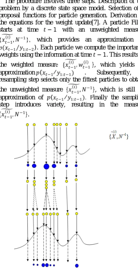
Among in the pictorial representation the random measures and actual probability distributions of interest are stated in three steps of the particle filtering [6]. They are Particle representation, Weight update and Re-sampling. Solid curves represent distributions of interest, which are approximated by discrete measures. The sizes of particles reflect the weights that are assigned to them.

The procedure involves three steps. Description of the problem by a discrete state space model. Selection of a proposal functions for particle generation. Derivation of the equations for the weight update[7]. A particle Filter starts at time − 1 with an unweighted measure { ( ) , }, which provides an approximation of ( ⁄ : ). Each particle we compute the importance weights using the information at time − 1. This results in the weighted measure { ( ) , ( ) }, which yields an approximation ( ⁄ _: ) . Subsequently, a resampling step selects only the fittest particles to obtain the unweighted measure { ( ) , }, which is still an approximation of ( ⁄ _: ). Finally the sampling step introduces variety, resulting in the measure { ( ) , }.

Fig. Pictorial representation of particle filter

Flow chart of particle filter:

The flow chart of particle filter is shown below [8,6].

Fig. Flow Chart of particle filter

Algorithm:

STEP–1: Initialize the weights of the states. STEP–2: Partitioning the individual weights. STEP–3: Normalize the updated weights. STEP–4: Estimate the desired unknown values. STEP–5: Get the output

STEP–6: If estimations fail go for more observations If Yes

Evaluate the particular particle size If necessary, go for re-sampling. If no, go for new observations. If No,

If evaluation not possible, go for exit.

Operation of Particle Filtering:

Particle filters are recursive implementation of Monte-Carlo based statistical signal processing. They approximate the optimal solution numerically based on physical model rather than applying an optimal filter. Particle filters are approximately the Bayesian posterior probability density function with a set of randomly chosen weighted samples. Each sample of a state vector is referred to as a particle.

Consider a system with a state space representation given by [8,6]

= ( , ) (5)

state vector at time instant t, state transition function, process noise with known distribution

= ( , ) (6)

The main task of sequential signal processing is the estimation of the state recursively from the observations . All the information about regarding filtering predicting or smoothing is captured by probability distribution functions. So the main goal is that tracking, which is obtaining

: from : .Practical

(4)

Generation of Particles:

For the joint a posterior distribution of , , … … . in case of independent noise samples which are assumed through out the particle.

:

: ∝ ∏ ( / ) ( / ) (7)

A recursive formula for obtaining

: from : is given by

: : =

( / ) ( / )

( / : ) ( : / : ) (8) Since the transition from ( / _: ) to :

: is often analytically intractable. In particle filtering, the distributions are approximated by discrete random measures defined by particles and weights assigned to the particles.

If the distribution of interest is P(x) and its approximating random measure is

= { ( )_, ( )_} ₍₉₎

( )_{are the particles and} ( )_{are the weights of particles,} m is the number of particles used in approximation. Approximates distribution ( )by

( ) = ∑ ( ) _{( −} ( )₎₍₁₀₎

Where is the dirac delta function. With this approximation, computations of expectations are simplified to summations.

Importance Sampling:

Importance sampling is choosing a good distribution from which to simulate one’s random variables.It involves multiplying the integrand by 1 to yield an expectation of quantity that varies less than the original integrand over the region of integration. The objective of importance sampling is aimed to sample the distribution in the region of importance in order to achieve computational efficiency. For the high dimensional space where the data are usually sparse and the region of interest where the target lies in relatively small in the whole data space. The idea of importance sampling to choose a proposal distribution ( ) in place of the probability distribution( ), which is hard to simple. Ideally the samples are generated directly from ∏( ).To generate from a density q(x) which is similar to∏( ).

The pdf ( ) is referred to as importance or proposal density. It is similar to∏( )and can be expressed by the following condition [9]

∏( ) > 0 ⟹ ( ) > 0 for all ∈

Here ( )and ∏( )have the same support. The above condition is necessary for the importance sampling theory to be hold and if valid, any integral of the form[10],

= ( ) ∏( ) = ∫ ( )∏( )_{( )} ( ) (11) A Monte Carlo estimate of I is computed by generating

>> 1independent samples.

{ ; = 1, . . . , }distributed according to ( ) and forming the weighted sum.

= ∑ ( ) ( ) (12)

Where ( ) =∏( )

( ) (13)

If the normalizing factor of the desired density∏(x)is unknown.

Then normalization of importance weights is performed then

= ∑ _∑ ( ) ( )_{( )} = ∑ ( ) ( ) (14) When the normalized importance weights are given by

( ) =_∑ ( )_{( )} (15)

This method of wisely choosing a pdf that corresponds to the integrand f is called importance sampling. In effect, it generates more random samples in areas where the value of f is high and fewer samples f is smaller.

Re-Sampling:

Re-sampling usually occurs between two importance sampling steps. In re-sampling step, the particles and associated importance weights{ , }are replaced by the new samples with equal importance weights. Whenever a significant degeneracy is observed, re-sampling is required in the sis algorithm. Re-sampling eliminates samples with low importance weights and multiples samples with high importance weights[11]. Measure of degeneracy of the algorithm is the effective sample size introduced in Kong, Liu and Wong[12] and Liu[13] and defined as:

=

. _: ( ∗( : )) (16) =

. _: [( ∗( : )) ] ≤ (17) It must cannot evaluate exactly, but an estimate

and is given by[14] =

∑ ( ) (18)

When is below a fixed threshold, the SIR resampling procedure is used.

It involves a mapping of random measure{ , } into random measure with uniform weights. The new set of random samples are generated by re-sampling N times from an approximate discrete representation of ( / ) given by

The resulting sample is a sample from the discrete density and hence the new weights are uniform. Although the re-sampling step reduces the effects of the degeneracy problem. This leads to a loss of diversity among the particles as the resultant sample will contain many repeated points. This problem is known as sample impoverishment, is severe in the case of small process noise. In fact, for the case of very small process noise, all particles will collapse to a single point within little iteration. To solving the problem of sample impoverishment is the resample move algorithm. This technique draws conceptually o the same technologies of importance sampling-re-sampling and MCMC sampling, it avoids sample impoverishment.

V. R

ESULTS

(5)

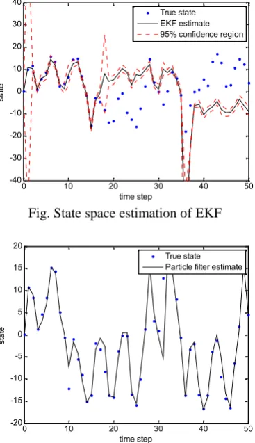
and Particle filtering approaches. Figure one shows that the Kalman filtering approach resultant, the second one shows that the filtering approach of the Extended Kalman Filtering approach resultant and the third one shows that the Particle filtering approach of state apace approach.

Fig. State estimation using particle filter & Kalman

Fig. State space estimation of EKF

Fig. State Space estimation of Particle Filtering While estimating the state space modelling using several filtering approaches practically we got the result as the best result of particle filtering approaches. While observing the above three graphical representations we easily identifies that the resultant approach of all filters particle filter having the highest probability density

function of state space estimation per unit area. So, while comparing with all the other filtering approaches of state space estimation particle filtering approach is good and gives better performance.

VI. C

ONCLUSION

We considered a set of equations which consists of non-linear and non-gaussian functions and represented in a state space model, where first equation representation the state of the system and second equation represents the measurement equation. Particle filtering algorithm is applied to this set of equations in order to eliminate the problems regarding non-linear and non-gaussian functions. The simulation results are observed from the particle filtering algorithm which involves the sequential importance sampling and re-sampling. For the better estimates of the states, the posterior mean estimate and Maximum a Posterior Estimate (MAP) of samples are observed. This convergence proof clearly shows that this algorithm can lead to substantial improvements over other non-linear filtering algorithms.

R

EFERENCES

[1] Greg Welch, and Gary Bishop, ”An Introduction to the Kalman

Filter”. Siggraph 2001, Course 8.

[2] Mohinder S. Grewal, Angus P. Andrews, “Kalman Filtering:

Theory and Practice Using MATLAB”. Second edition.

[3] Fredrick Orderud, “Comparsion of Kalman filter Estimation

Approaches for State Space Models with Nonlinear

Measurements”. Sem Saelands Vei 7-9, NO-7491 Trondheim.

[4] Simon J.Julier, Jeffrey K.Uhlmann,“A NewExtension of the

Kalman Filter to Nonlinear Systems”.

[5] Yufei Huang, and Peter M.Djuric, “A Blind Particle Filtering

Detector of Signals Transmitted Over Flat Fading Channels”.

IEEE Transactions on Signal Processing, Vol .52, NO 7,July 2004.

[6] Petar M.Djuric, Jayesh H.Kotecha, Jianqui Zhang, Yufei Huang, Tadesse Ghirmai, Monica F.Bugallo, Joaquin Miguez,

”Applications of particle filtering to selected problems in communications”. Submitted to IEEE Signal Processing

Magazine.

[7] Rudolph Vander Merwe, Arnaud Doucet, Nando de Freitas, Eric

Wan, “The Unscented Particle Filter”.

[8] Petar M.Djuric, Jayesh H.Kotecha, Jianqui Zhang, Yufei Huang,

Tadesse Ghirmai, Monica F.Bugallo, Joaquin Miguez, “Particle

filtering: A Review of the theory and how it can be used for

soling problems in wireless communications”.IEEE Signal

Proceesing Magazine.

[9] Nicolas Bergman, “Recursive Bayesian Estimation”. Navigation

and Tracking Applications

[10] ZHE CHEN, “Bayesian filtering: From Kalman Filters to

Particle Filters, and Beyond”.

[11] Arnaud Doucet, Simon Godsill and Christophe Andrieu, “On

Sequential Monte Carlo Sampling Methods for Bayesian

Filtering”. Statistics and Computing (2000) 10, 197-208.

-40 -30 -20 -10 0 10 20 30 40

0 0.05 0.1 0.15 0.2 0.25 0.3 0.35 0.4 0.45

0.5 Estimated pdf at k=20

Particle filter Kalman filter

0 10 20 30 40 50

-40 -30 -20 -10 0 10 20 30 40

time step

st

at

e

True state EKF estimate 95% confidence region

0 10 20 30 40 50

-20 -15 -10 -5 0 5 10 15 20

time step

st

at

e