A conservative numerical scheme for Rosenau-RLW equation based on multiple integral finite volume method

R E S E A R C H

Open Access

A conservative numerical scheme for

Rosenau-RLW equation based on multiple

integral finite volume method

Cui Guo

1*

_{, Fang Li}

1

_{, Wenping Zhang}

1

_{and Yuesheng Luo}

1

*_{Correspondence:}

2185835@163.com

1_{Harbin Engineering University,}

Harbin, P.R. China

Abstract

A multiple integral finite volume method combined and Lagrange interpolation are applied in this paper to the Rosenau-RLW (RRLW) equation. We construct a two-level implicit fully discrete scheme for the RRLW equation. The numerical scheme has the accuracy of third order in space and second order in time, respectively. The solvability and uniqueness of the numerical solution are shown. We verify that the numerical scheme keeps the original equation characteristic of energy conservation. It is proved that the numerical scheme is convergent in the order ofO(

τ

2_+h3_{) and}

unconditionally stable. A numerical experiment is given to demonstrate the validity and accuracy of scheme.

Keywords: Multiple integral finite volume method; Rosenau-RLW equation; Lagrange interpolation; Brouwer fixed point theorem

1 Introduction

It is well known that nonlinear partial differential equations exist in many areas of mathe-matical physics and fluid mechanics. In the nonlinear evolution equations, the Korteweg– de Vries (KdV) and Rosenau-RLW (RLW) equations are two typical cases, given by

ut+uxxx+uux= 0 (1.1)

and

ut–uxxt+ux+uux= 0. (1.2)

The KdV equation (1.1) is a nonlinear model used to study the change forms of long waves propagating in a rectangular channel. The RLW equation (1.2) is used to simulate wave motion in media with nonlinear wave steeping and dispersion. The RLW equation was proposed by Peregrine [1,2] based on the classical KdV equation, and an explanation of different situations of a nonlinear dispersive wave was given in his research.

At the same time, we notice that the motion described by the RLW equation has the same approximate boundary as the KdV equation. It is well known that the KdV equation has corresponding shortcomings. With the aim to overcome these unavoidable shortcomings

of the KdV equation, Rosenau [3,4] introduced an equation

ut+uxxxxt+ux+uux= 0. (1.3)

The theoretical studies, on the existence, uniqueness and regularity for the solution of (1.3), have been performed by Park [5]. Various numerical techniques have been used to solve the Rosenau equation [6–12], particularly including the discontinuous Galerkin method, the C1-conforming finite element method [13], the finite difference method and the orthogonal cubic spline collocation method. More detailed solving processes can be obtained in Refs. [14–19].

On the other hand, for further understanding more general nonlinear behaviors of the waves, the term –uxxtneeds to be considered. So we address

ut–uxxt+uxxxxt+ux+uux= 0. (1.4)

This equation is usually called the Rosenau-RLW (RRLW) equation. Zuoet al. [20] pro-posed a Crank–Nicolson finite difference method for the RRLW equation. Meanwhile, a three-level difference scheme for (1.4) is investigated by Panet al. [21]. Furthermore, the finite element approximate solution is used to solve (1.4) and related error estimations for both semi-discrete and fully discrete Galerkin methods are established [22–24]. The coupling equation of KdV and RRLW is also solved through a three-level average implicit finite difference scheme, showing second-order accuracy in space and time, simultane-ously [25]. In Ref. [26], the Galerkin cubic B-spline finite element method is proposed to construct the numerical scheme for the RRLW equation. Pan [27] investigated the C-N scheme of RRLW equation through a more classic finite difference approach, and corre-sponding solvability and convergence have been proved. In addition, the difference scheme for the general RRLW equation is constructed by Wang [28] with some theoretical proofs. The main contribution of the current work is to present a two-level implicit numerical scheme for the following RRLW equation with some theoretic analysis:

ut–uxxt+uxxxxt+ux+uux= 0, (x,t)∈(xl,xr)×[0,T] (1.5)

with the initial condition

u(x, 0) =u0(x), x∈[xl,xr] (1.6)

and boundary conditions

u(xl,t) =u(xr,t) = 0, uxx(xl,t) =uxx(xr,t) = 0, t∈[0,T]. (1.7)

Throughout this paper, we assume that the initial conditionu0(x) is sufficiently smooth as required by the error analysis. The system (1.5)–(1.7) is known to satisfy the following conservative law:

The contents of this paperis as follows. Firstly, in Sect.2, we present some notations and lemmas. In Sect.3, we propose a multiple integral finite volume method which is a tool for discrete partial differential equations. Thus a two-level implicit numerical scheme for the RRLW equation is obtained. Next we discuss the discrete energy conservative laws of the numerical scheme and prove its solvability and uniqueness in Sect.3. We give prior estimates of the numerical scheme in Sect.4and prove that the numerical scheme is con-vergent and stable in Sect.5. Finally, the error analysis and energy analysis of numerical examples are given in Sect.6.

In fact, the numerical discrete scheme with parameters constructed by us shows all the discrete schemes that can be constructed by the finite difference method. By choosing the undetermined parameters, we find the best discrete scheme. The best discrete scheme can preserve the conservation property of the original differential equation well. At the same time, for unknown functions in the original differential equation, this method reduces greatly the requirements for the unknown functions in terms of mathematics. More im-portantly, we explain the concrete and detailed methods about improving the accuracy of the numerical discrete scheme.

2 Some notations and lemmas 2.1 Some notations

Lethandτ be the uniform step sizes in the spatial direction and temporal direction, re-spectively, wheref =xr–xl

J andτ= T N.

Denotexj=xl+jh(0≤j≤J),tn=nτ (0≤n≤N) andun

j ≈u(xl+jh,nτ). Denote the gridΩh={xj|j= 0, 1, . . . ,J}andZ0h={uj|u0=uJ= 0,j= 0, 1, . . . ,J}. As usual, the following notations will be used:

un+

1 2

j

t= un+1

j –unj

τ , u

n+1₂

j =

un+1 j +unj

2 ,

un_jx=u n j+1–unj

h ,

un_jx=u n j –unj–1

h ,

un_jx=u n j+1–unj–1

2h ,

un_jxx=un_jxx=u n

j+1– 2unj +unj–1 h2 ,

un+

1 2

j

xxxx= un+

1 2

j–2 – 4u n+1₂ j–1 + 6u

n+1₂ j – 4u

n+1₂ j+1 +u

n+1₂ j+2

h4 ,

un,vn=h j

un_jvn_j,

un=un_,un_{, u}n

∞=₀max_≤j≤Junj.

In this paper we denote byCa positive constant, which may be of different values on different occasions.

2.2 Some lemmas

Lemma 2.1 For any two mesh functions u,v∈Z0

h,we have

(ux,v) = –(u,vx), (uxx,v) = –(ux,vx), (uxx,u) = –(ux,ux) = –ux2.

Lemma 2.2 2B–E is a positive definite matrix,where matrix E is the identity matrix of order J+ 1and

B=

⎡ ⎢ ⎢ ⎢ ⎢ ⎢ ⎢ ⎢ ⎢ ⎢ ⎢ ⎢ ⎣

1 0 0 · · · 0 0 0 0 7 1 · · · 0 0 0 0 1 7 · · · 0 0 0

..

. ... ... . .. ... ... ... 0 0 0 · · · 7 1 0 0 0 0 · · · 1 7 0 0 0 0 · · · 0 0 1

⎤ ⎥ ⎥ ⎥ ⎥ ⎥ ⎥ ⎥ ⎥ ⎥ ⎥ ⎥ ⎦

(J+1)×(J+1) .

Proof We know that

2B–E=

⎡ ⎢ ⎢ ⎢ ⎢ ⎢ ⎢ ⎢ ⎢ ⎢ ⎢ ⎢ ⎣

1 0 0 · · · 0 0 0 0 13 2 · · · 0 0 0 0 2 13 · · · 0 0 0

..

. ... ... . .. ... ... ... 0 0 0 · · · 13 2 0 0 0 0 · · · 2 13 0 0 0 0 · · · 0 0 1

⎤ ⎥ ⎥ ⎥ ⎥ ⎥ ⎥ ⎥ ⎥ ⎥ ⎥ ⎥ ⎦

(J+1)×(J+1) .

LetB1= [1],B2=

_{1 0}

0 13

,B3=

_{1 0 0}

0 13 2 0 2 13

,BJ+1= 2B–E. It is obvious that|B1|= 1 > 0,|B2|= 13 > 0,|B3|= 165 > 0 and{|Bj|}(j= 4, . . . ,J) obeys

|Bj|= 13|Bj–1|–|Bj–2|+|Bj–3|.

We can get

|B4|= 13|B3|–|B2|+|B1|,

|B5|= 13|B4|–|B3|+|B2|,

· · ·

|BJ|= 13|BJ–1|–|BJ–2|+|BJ–3|.

(2.1)

We assume that|B1|,|B2|, . . . ,|BJ–1|> 0. We want to prove|BJ|> 0. From (2.1),

|BJ|= 12|BJ–1|+· · ·+|B3|

–|BJ–2|+|B3|+|B1|

= 11|BJ–1|+· · ·+|B3|

+|BJ–1|+|BJ–3|+· · ·+|B3|

+ 166 > 0. (2.2)

By the assumption, we have

|BJ+1|=|BJ|> 0.

Lemma 2.3(Fixed point theorem [29]) H is a finite dimensional inner product space.We assume g:H→H and g is continuous.If there existsα> 0,for any x in H,as long asx=

α,we have(g(x),x) > 0.Then there must exist x∗∈H(x∗ ≤α),which obeys g(x∗) = 0.

Lemma 2.4(Discrete Sobolev’s inequality [29]) For any discrete function uhand for any givenε> 0,there exists a constant K(ε,n),depending only onεand n,such that

u∞≤εun_x+K(ε,n)un.

Lemma 2.5(Discrete Gronwall’s inequality [30]) Suppose that the discrete function wh satisfies the recurrence formula

wn–wn–1≤Aτwn+Bτwn–1+Cnτ,

where A,B,Cn(n= 1, 2, . . . ,N)are nonnegative constants.Then

wn∞≤

w0+τ N

k=1 Ck

e2(A+B)τ_,

whereτ is small,such that(A+B)τ≤N_2N–1(N> 1).

3 An implicit conservative numerical scheme and its discrete conservative law 3.1 The multiple integral finite volume method

It is necessary to introduce the multiple integral finite volume method (MIFVM) briefly. The method is a new approximation method for solving partial differential equation, which is proposed by Yuesheng Luo. The basic idea is to make the original partial dif-ferential equation to be an integral equation by a certain number of integrations in the spatialxdirection. The goal is that the integral equation no longer contains the deriva-tive item of the unknown function. In this way, we avoid handling the approximation as regards the derivative term.

Firstly, the number of integrations depends on the order of the highest derivative in the spatialxdirection of the unknown function in the partial differential equation. The rela-tionship betweenmandrsatisfiesm= 2r– 1, wheremis the number of integrations and ris the order of the highest derivative of the unknown function in the spatialxdirection. Secondly, is it well known that the original partial differential equation usually is ex-pressed by the derivative of an unknown function and an unknown function, for example ux,uxx,uxxx,uxxxxandu. The MIFVM is to transform the original partial differential equa-tion into an integral equaequa-tion, which is expressed byun_j.un_j ≈u(xl+jh,nτ) is the unknown function’s approximate value at the grid node. If there isun

j+ε, which is not at the grid node,

in the integral equation, we often use the Lagrange polynomial to deal with it. This step is just an approximation to the original function.

For example, for (1.5), the order of the highest derivative of unknown function is four. Bym= 24– 1, we should make 15 times integrations for every item, as shown by

xxxx ut–

xxxx uxxt+

xxxx uxxxxt+

xxxx ux+

xxxx

where

xxxx udef=

xj+ε8

xj+ε7

dxf2 xj+ε7

xj+ε6

dxf1 xj+ε6

xj+ε5

dxe2 xj+ε5

xj

dxe1

× xj

xj–ε4

dxd2 xj–ε4

xj–ε3

dxd1 xj–ε3

xj–ε2

dxc2

× xj–ε2

xj–ε1

dxc1 xf2

xf₁

dxf

xe₂

xe₁

dxe

xd2

xd₁

dxd

xc₂

xc₁

dxc × xf xe dxb xd xc dxa xb xa

u dx, (3.2)

εi∈R,i= 1, 2, . . . , 8. The center difference is used to deal with the first derivative in the time direction. Then we can get a numerical scheme for the original equation.

3.2 A two-level implicit numerical scheme

In order to get a numerical scheme, which can preserve some properties of the original equation, applying MIFVM to Eq. (1.5) on timen+1

2 level, we letε1= –ε4= –ε5=ε8=

√

3h,ε2= –ε3= –ε6=ε7=

√

3

3 h. So we can get

xj+

√

3h

xj+

√

3 3 h

dxf2 xj+

√

3 3 h

xj–

√

3 3h

dxf1 xj–

√

3 3 h

xj–

√

3h dxe2

xj

xj–

√

3h dxe1

xj+

√

3h

xj

dxd2

× xj+

√

3h

xj+

√

3 3 h

dxd1 xj+

√

3 3 h

xj–

√

3 3 h

dxc2 xj–

√

3 3 h

xj–

√

3h dxc1

× xf2

xf1

dxf

xe2

xe1

dxe

xd2

xd1

dxd

xc2

xc1

dxc xf xe dxb xd xc dxa xb xa utdx –

xj+

√

3h

xj+

√

3 3 h

dxf2 xj+

√

3 3 h

xj–

√

3 3 h

dxf1 xj–

√

3 3 h

xj–

√

3h dxe2

xj

xj–

√

3h dxe1

xj+

√

3h

xj

dxd2

× xj+

√

3h

xj+

√

3 3 h

dxd1 xj+

√

3 3 h

xj–

√

3 3 h

dxc2 xj–

√

3 3 h

xj–

√

3h dxc1

× xf2

xf₁

dxf

xe₂

xe₁

dxe

xd2

xd₁

dxd

xc₂

xc₁

dxc xf xe dxb xd xc dxa xb xa uxxtdx +

xj+

√

3h

xj+

√

3 3 h

dxf2 xj+

√

3 3 h

xj–

√

3 3h

dxf1 xj–

√

3 3 h

xj–

√

3h dxe2

xj

xj–

√

3h dxe1

xj+

√

3h

xj

dxd2

× xj+

√

3h

xj+

√

3 3 h

dxd1 xj+

√

3 3 h

xj–

√

3 3 h

dxc2 xj–

√

3 3 h

xj–

√

3h dxc1

× xf₂

xf1

dxf

xe2

xe1

dxe

xd₂

xd1

dxd

xc2

xc1

dxc xf xe dxb xd xc dxa xb xa uxxxxtdx +

xj+

√

3h

xj+

√

3 3 h

dxf2 xj+

√

3 3 h

xj–

√

3 3h

dxf1 xj–

√

3 3 h

xj–

√

3h dxe2

xj

xj–

√

3h dxe1

xj+

√

3h

xj

dxd2

× xj+

√

3h

xj+

√

3 3 h

dxd1 xj+

√

3 3 h

xj–

√

3 3 h

dxc2 xj–

√

3 3 h

xj–

√

× xf₂

xf₁

dxf

xe2

xe1

dxe

xd₂

xd₁

dxd

xc2

xc1

dxc xf xe dxb xd xc dxa xb xa uxdx +

xj+

√

3h

xj+

√

3 3 h

dxf2 xj+

√

3 3 h

xj–

√

3 3h

dxf1 xj–

√

3 3 h

xj–

√

3h dxe2

xj

xj–

√

3h dxe1

xj+

√

3h

xj

dxd2

× xj+

√

3h

xj+

√

3 3 h

dxd1 xj+

√

3 3 h

xj–

√

3 3 h

dxc2 xj–

√

3 3 h

xj–

√

3h dxc1

× xf2

xf1

dxf

xe2

xe1

dxe

xd2

xd1

dxd

xc2

xc1

dxc xf xe dxb xd xc dxa xb xa

uuxdx= 0. (3.3)

There are five integration items. For the first item, the approximation of the first-order derivative in the time direction is

utx,tn+12₌u

n+1_{(x) –u}n_(x)

τ +O

τ2. (3.4)

For the third item, we use the five points Lagrange interpolation for thexdirection. It is

u(x,t) = (x–xj–1)(x–xj)(x–xj+1)(x–xj+2) (xj–2–xj–1)(xj–2–xj)(xj–2–xj+1)(xj–2–xj+2)

uj–2(t)

+ (x–xj–2)(x–xj)(x–xj+1)(x–xj+2) (xj–1–xj–2)(xj–1–xj)(xj–1–xj+1)(xj–1–xj+2)

uj–1(t)

+ (x–xj–2)(x–xj–1)(x–xj+1)(x–xj+2) (xj–xj–2)(xj–xj–1)(xj–xj+1)(xj–xj+2)

uj(t)

+ (x–xj–2)(x–xj–1)(x–xj)(x–xj+2) (xj+1–xj–2)(xj+1–xj–1)(xj+1–xj)(xj+1–xj+2)

uj+1(t)

+ (x–xj–2)(x–xj–1)(x–xj)(x–xj+1) (xj+2–xj–2)(xj+2–xj–1)(xj+2–xj)(xj+2–xj+1)

uj+2(t) +O

h5. (3.5)

For the other three items, we use three points Lagrange interpolation for thexdirection. It is

u(x,t) = (x–xj)(x–xj+1) (xj–1–xj)(xj–1–xj+1)

uj–1(t) +

(x–xj–1)(x–xj+1) (xj–xj–1)(xj–xj+1)

uj(t)

+ (x–xj–1)(x–xj) (xj+1–xj–1)(xj+1–xj)

uj+1(t) +O

h3. (3.6)

Substituting (3.4), (3.5) and (3.6) into (3.3) and simplifying, we get a two-level implicit scheme for equation (1.5). We obtain

1 9

un+

1 2

j–1 + 7u n+1₂ j +u

n+1₂ j+1

t–

un+

1 2

j

xxt+

un+

1 2

j

xxxxt+

un+

1 2 j x +1 3

un+

1 2 j x

un+

1 2

j–1 +u n+12

j +u n+12

j+1

= 0, 1≤j≤J– 1, 1≤n≤N– 1, (3.7)

u0_j =u0(xj), 1≤j≤J– 1, (3.8)

3.3 Conservative law of the discrete format

Theorem 3.1 The two-level implicit numerical scheme(3.7)admits the following invari-ant:

En=7 9u

n2₊2h 9

J–1

j=1

un_jun_j+1+un_x2+un_xx2=En–1=· · ·=E0.

Proof Computing the inner product of (3.7) with 2un+12 _{(i.e. u}n+1 _+un_{), according to}

Lemma2.1, we have

7 9τu

n+12 +2h

9τ

J–1

j=1

un_j+1un_j+1+1– 7 9τu

n2 +2h

9τ

J–1

j=1

un_jun_j+1+1

τu

n+1

x

2

–un_x2

+1

τu

n+1 xx

2

–un_xx2+P, 2un+12_{= 0, (3.10)}

whereP= 1₃(un+

1 2

j )x(u n+1₂ j–1 +u

n+1₂ j +u

n+1₂

j+1 ). Now, computing the last term of the left-hand side in (3.10), we get

P, 2un+12

=

2 3

un+

1 2 j x

un+

1 2

j–1 +u n+1₂ j +u

n+1₂ j+1

,un+12 =1 3 J–1 j=1

un+

1 2

j+1 u n+12

j u n+12

j +u n+12

j+1 u n+12

j u n+12

j+1 –u n+12

j–1 u n+12

j u n+12

j–1 –u n+12

j–1 u n+12

j u n+12

j =1 3 _J–2 j=1

un+

1 2

j u n+12

j u n+12

j+1 +u n+12

j u n+12

j+1 u n+12

j+1 –u n+12

j u n+12

j u n+12

j+1 –u n+12

j u n+12

j+1 u n+12

j+1

+un+

1 2

J–1u n+1₂ J–1u

n+1₂ J +u

n+1₂ J–1 u

n+1₂ J u

n+1₂ J

–un+

1 2

0 u n+1₂ 0 u

n+1₂ 1 +u

n+1₂ 0 u

n+1₂ 1 u

n+1₂ 1

= 0. (3.11)

Substituting (3.11) into (3.10), we have

7 9u

n+12₊2h 9

J–1

j=1

un_j+1un_j+1+1–7 9u

n2

+2h 9

J–1

j=1

un_jun_j+1+un_x+12–u_xn2+un_xx+12–un_xx2= 0.

We let

En=7 9u

n2₊2h 9

J–1

j=1

Then we obtain

En₌7 9u

n2₊2h 9

J–1

j=1 un

junj+1+unx 2

+un xx

2

=En–1_{=· · ·=E}0_{. (3.12)}

The proof is completed.

3.4 Solvability

Next, we shall prove the solvability of the difference scheme (3.7).

Theorem 3.2 The finite difference scheme(3.7)is solvable.

Proof For the difference scheme (3.7)–(3.9), we assume thatu0,u1, . . . ,un(n≤N– 1) obey (3.7). Next, we will prove thatun+1also satisfies (3.7). The operationgis defined as follows:

g(v) =2 9A

v–un– 2vxx–u_xxn+ 2vxxxx– 2un_xxxx+τvx+

τ

3(vj–1+vj+vj+1)vx. (3.13)

It is obvious thatgis continuous. Computing the inner product of (3.13) withv, accord-ing to Lemma2.1, we have

g(v),v=2 9(Av,v) –

2 9

Aun,v– 2(vxx,v) + 2un_xx,v+ (2vxxxx,v) –2un_xxxx,v

≥2

9v

T_WT_v+2 9v

T_LT_v–2 9Au

n_{v+ 2vx}2

– 2un_xvx+ 2vxx2– 2un_xxvxx

≥2

9

λ0v20+λ2v21+· · ·+λJv2J

–1 9Au

n2

–1 9v

2_+vx2_–un x

2

+vxx2–un_xx2

≥1

9(2λmin– 1)v 2_–1

9Au n2

–un_x2–un_xx2,

where

A=

⎡ ⎢ ⎢ ⎢ ⎢ ⎢ ⎢ ⎢ ⎢ ⎢ ⎢ ⎢ ⎣

1 0 0 · · · 0 0 0 1 7 1 · · · 0 0 0 0 1 7 · · · 0 0 0

..

. ... ... . .. ... ... ... 0 0 0 · · · 7 1 0 0 0 0 · · · 1 7 1 0 0 0 · · · 0 0 1

⎤ ⎥ ⎥ ⎥ ⎥ ⎥ ⎥ ⎥ ⎥ ⎥ ⎥ ⎥ ⎦

(J+1)×(J+1)

W= ⎡ ⎢ ⎢ ⎢ ⎢ ⎢ ⎢ ⎢ ⎢ ⎢ ⎢ ⎢ ⎣

1 0 0 · · · 0 0 0 0 7 1 · · · 0 0 0 0 1 7 · · · 0 0 0

..

. ... ... . .. ... ... ... 0 0 0 · · · 7 1 0 0 0 0 · · · 1 7 0 0 0 0 · · · 0 0 1

⎤ ⎥ ⎥ ⎥ ⎥ ⎥ ⎥ ⎥ ⎥ ⎥ ⎥ ⎥ ⎦

(J+1)×(J+1) , L= ⎡ ⎢ ⎢ ⎢ ⎢ ⎢ ⎢ ⎢ ⎢ ⎢ ⎢ ⎢ ⎣

0 0 0 · · · 0 0 0 1 0 0 · · · 0 0 0 0 0 0 · · · 0 0 0

..

. ... ... . .. ... ... ... 0 0 0 · · · 0 0 0 0 0 0 · · · 0 0 1 0 0 0 · · · 0 0 0

⎤ ⎥ ⎥ ⎥ ⎥ ⎥ ⎥ ⎥ ⎥ ⎥ ⎥ ⎥ ⎦

(J+1)×(J+1) ,

λminis the minimum eigenvalue ofW. By Lemma2.2, we know that 2λmin– 1 > 0. Let

v2= 1 2λmin– 1

_Aun2_{+ 9u}n x

2

+ 9un_xx2+ 1.

We have (g(v),v) > 0,∀v∈Z0_h. According to Lemma2.3, there isv∗∈Z0_h which obeys g(v∗) = 0. So we letv∗=un+1₂+un, thenun+1_{obeys (3.7).}

Theorem 3.3 The finite difference scheme(3.7)has a unique solution.

Proof LetIn+1_=Un+1_–Vn+1_{, whereU}n+1_andVn+1_{are both the solution of scheme (3.7).} We want to prove thatIn+1= 0. According to (3.7), we get

1 9

In+

1 2

j–1

t+ 7

In+

1 2 j t+

In+

1 2 j+1 t

–In+

1 2

j

xxt+

In+

1 2

j

xxxxt+

In+

1 2

j

x

+ϕun+

1 2

j ,u n+1₂ j

–ϕvn+

1 2

j ,v n+1₂ j

= 0, (3.14)

where ϕ(un+

1 2

j ,u n+1₂ j ) = 13(u

n+1₂ j )x(u

n+1₂ j–1 +u

n+1₂ j +u

n+1₂

j+1 ). Computing the inner product of (3.12) with 2In+12_(In_+In+1_{), we have}

7 9τI

n+12 +2h

9τ

J–1

j=1

I_jn+1I_jn₊₁+1– 7 9τI

n_–2h 9τ

J–1

j=1 I_jnI_jn₊₁

+1

τI

n+1

x

2

–I_xn2+1

τI

n+1 xx

2

–I_xxn2

+ϕun+

1 2

j ,u n+1₂ j

–ϕvn+

1 2

j ,v n+1₂ j

,In+12_{= 0.}

Due to the result that

–ϕun+

1 2

j ,u n+12

j

–ϕvn+

1 2

j ,v n+12

j

= –2 3h J–1 j=1

In+

1 2

j–1 +I n+1₂ j +I

n+1₂ j+1

un+

1 2

j

xI n+1₂ j –2 3h J–1 j=1

In+

1 2

j–1 +I n+1₂ j +I

n+1₂ j+1

vn+

1 2

j

xI n+1₂ j –2 3h J–1 j=1

vn+

1 2

j–1 +v n+1₂ j +v

n+1₂ j+1

un+

1 2

j

xI n+1₂ j +2 3h J–1 j=1

un+

1 2

j–1 +u n+1₂ j +u

n+1₂ j+1

vn+

1 2

j

xI n+1₂ j ≤2 3Ch J–1 j=1

_In+12

j–1 +I n+12

j +I n+12

j+1 I n+12

j + 2 3Ch

J–1

j=1

In+

1 2

j

xI n+12

j

≤CIn+12+In2+I_xn+12+I_xn2,

we have

7 9τI

n+12 +2h

9τ

J–1

j=1

I_jn+1I_jn₊₁+1– 7 9τI

n2 –2h

9τ

J–1

j=1 I_jnI_jn₊₁

+1

τI

n+1

x

2

–I_xn2+1

τI

n+1 xx

2

–I_xxn2

≤CIn+12+In2+I_xn+12+I_xn2.

Let

Qn=7 9I

n2 +2h

9 J–1

j=1

I_jnI_jn₊₁+I_xn2+I_xxn2.

So we get

Qn+1–Qn≤CτQn+1+Qn.

That is,

Qn+1≤1 +Cτ 1 –CτQ

n_{= (1 +ϑ τ)Q}n_,

whereϑ= 2C

1–Cτ. Then we have

Qn+1≤(1 +ϑ τ)Qn≤ · · · ≤(1 +ϑ τ)n+1Q0≤ · · · ≤eϑ τ(n+1)Q0.

BecauseQ0₌7 9I

02₊2h 9

J–1

j=1Ij0Ij0+1+Ix02+Ixx02= 0,Qn+1≤eϑ τ(n+1)Q0= 0. We have

Qn=7 9I

n2₊2h 9

J–1

j=1

It is well known that

5 9I

n+12

+I_xn+12+I_xxn+12≤Qn= 0.

SoIn+12_=Un+1_–Vn+12_{= 0. We can say thatU}n+1_=Vn+1_.

4 Some prior estimates for the difference solution

In this section, we shall make some prior estimates for the numerical scheme.

Theorem 4.1 Assume that u0∈H02[xl,xr]then there is the estimation for the solution of the numerical scheme(3.7)

un_xx≤C, u_xn≤C, un_∞≤C.

Proof It follows from (3.12) that

5 9u

n2₊

2 9u

n2₊2 9

J–1

i=1

un_iun_i+1h

+un_x2+un_xx2=C (4.1)

we obtain from (4.1) 5

9u n2

+un_x2+un_xx2≤C.

So

un_xx≤C, u_xn≤C, un≤C.

It follows from Lemma2.4thatun∞≤C. Remark4.1 Theorem4.1implies that the scheme (3.7)–(3.9) is unconditionally stable.

5 Convergence and stability of the difference scheme

Now, we consider the truncation error of scheme of (3.7). Firstly, we define the truncation error as follows:

Ern+

1 2

j =

1 9τ

vn_i–1+1+ 7v_in+1+vn_i+1+1–vn_i–1– 7vn_i –vn_i+1+vn+

1 2

i

x

–vn+

1 2

i

xxt+

vn+

1 2

i

xxxxt+ 1 3

vn+

1 2

i

x

vn+

1 2

i–1 +v n+1₂ i +v

n+1₂ i+1

. (5.1)

According to Taylor expansion and Lagrange interpolation, we obtain the following.

Lemma 5.1 Assume that u0∈H02[xl,xr]and u(x,t)∈C5,2,then the truncation errors of the numerical scheme(3.7)satisfy

Ern+

1 2

j =O

Theorem 5.1 Assume that u0∈H02[xl,xr]and u(x,t)∈C5,2,then the solution of the nu-merical scheme(3.7)converges to the solution of the initial-boundary value problem(1.5)– (1.7)with order O(τ2+h3_{)by the ·}

∞norm.

Proof Leten+

1 2

j =u(xj,tn+

1 2_{) –u}n+

1 2

j . Subtracting (3.7) from (5.1), we have Ern+

1 2 j = 1 9τ

en_j–1+1+ 7en_j+1+en_j+1+1–en_j–1– 7en_j –en_j+1+1 4

en_j+1_x+en_jx–en+

1 2

j

xxt

+en+

1 2

j

xxxxt+ 1 3

uxj,tn+12

x

uxj–1,tn+

1

2_+uxj,tn+12_+uxj

+1,tn+

1 2

–1 3

un+

1 2 j x

un+

1 2

j–1 +u n+1₂ j +u

n+1₂ j+1

. (5.3)

For simple notation, the last two terms of (5.3) are defined by Q=uxj,tn+

1 2

x

uxj–1,tn+

1 2_+ux

j,tn+

1 2_+ux

j+1,tn+

1 2

–1 3

un+

1 2 j x

un+

1 2

j–1 +u n+1₂ j +u

n+1₂ j+1

.

Computing the inner product of (5.3) with 2en+1_{2 (i.e.e}n+1_+en_{), we get}

Ern+

1 2

j , 2en+

1 2

= 7 9τe

n+12₊2h 9τ

J–1

j=1

en_j+1en_j+1+1– 7 9τe

n2_–2h 9τ

J–1

j=1

en_jen_j+1+1

τe

n+1

x

2

–en_x2

+1

τe

n+1 xx

2

–en_xx2+Q, 2en+12_{. (5.4)}

According to Theorem3.3, we obtain –Q, 2en+12≤_Cen+12_+en2_+en+1

x

2

+en_x2. (5.5)

In addition, obviously

Ern+

1 2

j , 2en+

1

2_=Ern+ 1 2

j ,en+1+en

≤Ern+122₊1

2e

n+12_+en2_.

Substituting (5.4) and (5.5) into (5.3), we have 7

9e n+12

+2h 9

J–1

j=1

en_j+1en_j+1+1–7 9e

n2 –2h

9 J–1

j=1 en_jen_j+1

+en_x+12–en_x2+en_xx+12–en_xx2

≤τErn+122₊τ

2e

n+12_+en2

+Cτen+12+en2+en_x+12+en_x2. (5.6)

So

(1 –Cτ)Bn+1–Bn≤τErn+122_{+ 2CτB}n_.

Ifτ is sufficiently small so that it satisfies 1 –Cτ=σ> 0, then

Bn+1–Bn≤CτErn+122_+CτBn_{. (5.7)}

Summing up (5.7) from 0 ton– 1, we have

Bn–B0≤Cτ

n–1

i=0

Eri+122_+Cτ

n–1

i=0 Bi.

Noticing, τn_i=0–1Eri+212≤_{nτmax0≤i≤n–1Er}i+122≤_T·_O(τ2_+h2₎2_,e0_{= 0. We get}

B0_{= 0.}

Hence, from Lemma2.5, we obtain

Bn≤Oτ2+h32.

That is,

7 9e

n2

+en_x2+en_xx2≤Oτ2+h32.

So

en≤Oτ2+h3, en_x≤Oτ2+h3, en_xx≤Oτ2+h3.

Using Lemma2.4, we geten

∞≤O(τ2+h3_).

Theorem 5.2 Under the conditions of Theorem5.1,the solution of the numerical scheme (3.7)is unconditionally stable by the · ∞norm.

6 Numerical experiment

In this section, we will calculate some numerical experiments to verify the correctness of our theoretical analysis in the above part.

Consider the following initial boundary value problem of the Rosenau-RLW equation:

ut–uxxt+uxxxxt+ux+uux= 0, (x,t)∈(0, 1)×(0,T) (6.1)

with the initial condition

u(x, 0) =x3(1 –x)3, x∈[0, 1] (6.2)

and boundary conditions

Table 1 Absolute error of numerical solution atτ= 0.02

x J= 10 J= 30 J= 50 J= 80

0.1 1.92E–08 1.03E–09 2.45E–10 3.45E–12

0.2 3.23E–08 1.63E–09 3.47E–10 5.25E–11

0.3 3.27E–08 1.52E–09 2.33E–10 1.66E–10

0.4 2.09E–08 7.95E–10 5.49E–11 3.21E–10

0.5 2.11E–09 2.30E–10 4.09E–10 4.69E–10

0.6 1.68E–08 1.23E–09 7.20E–10 5.70E–10

0.7 2.91E–08 1.87E–09 8.82E–10 5.84E–10

0.8 2.96E–08 1.86E–09 8.07E–10 4.85E–10

0.9 1.76E–08 1.14E–09 4.80E–10 2.76E–10

Table 2 Discrete energy values ath=τ= 0.02

t En En[21] En[20]

0.1 0.058374806402 0.058524796850 0.057831719901

0.2 0.058374806389 0.058524796915 0.057831712420

0.3 0.058374806373 0.058524796919 0.057831704931

0.4 0.058374806345 0.058524796957 0.057831697437

0.5 0.058374806324 0.058524796889 0.057831689928

0.6 0.0583748062860 0.058524796925 0.057831682415

0.7 0.058374806258 0.058524796877 0.057831674891

0.8 0.058374806217 0.058524796939 0.057831667363

0.9 0.058374806168 0.058524797018 0.057831659824

1.0 0.058374806107 0.058524797061 0.057831652277

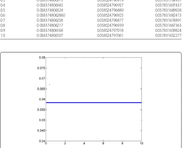
Figure 1Energy conservation properties of (3.7) atJ= 100,τ= 0.02,T= 10

Because we do not know the exact solution of (6.1)–(6.3), we consider the numerical solution of fine grid, takingh=₅₀₀1 , as the accurate solution of (6.1)–(6.3). Next we com-pare the numerical solution of the coarse grid and the numerical solution of fine grid. In order to obtain the error estimation, we consider the solution as a reference solution of the grid. In Table1, with the time stepτ= 0.02, we give the absolute error between numerical solution and accurate solution under a different spatial steph.

In Table2, withh=τ= 0.01, discrete energy values of numerical format (3.7) are given and are compared with the discrete energy values in the literature [20] and [21]. It can be seen that the multiple integral finite volume method preserves the conservation of discrete energy better than the numerical method in the literature [20] and [21]. Figure1shows the energy conservation properties of scheme (3.7) withJ= 100,τ= 0.02,T= 10.

7 Conclusion

In this paper, we have presented a two-level implicit nonlinear numerical scheme for the Rosenau-RLW equation, which has a wide range of applications in physics. The unique-ness, convergence and stability withO(τ2_+h3_{) of the numerical scheme were discussed} in detail. The scheme kept the energy conservation characteristic of the original equation. Finally, a numerical experiment shows that our scheme is efficient.

Acknowledgements

The authors wish to thank the referees for their valuable suggestions.

Funding

This work is supported by National Natural Science Foundation of China (NO. 11526064), Fundamental Research Funds for the Central Universities (NO. 3072019CF2403) and Graduate Education Fund (NO. 00211001060930).

Availability of data and materials

Data sharing not applicable to this article as no datasets were generated or analyzed during the current study.

Competing interests

The authors declare that they have no competing interests.

Authors’ contributions

All authors contributed equally and significantly in writing this article. All authors read and approved the final manuscript.

Authors’ information

The authors 1, 3 and 4 have been working at Harbin Engineering University for many years. The author Fang Li is a student. She has obtained her master degree of mathematics in Harbin Engineering University.

Publisher’s Note

Springer Nature remains neutral with regard to jurisdictional claims in published maps and institutional affiliations.

Received: 11 January 2019 Accepted: 2 October 2019

References

1. Peregrine, D.H.: Calculations of the development of an undular bore. J. Fluid Mech.25(2), 321–330 (1966) 2. Peregrine, D.H.: Long waves on a beach. J. Fluid Mech.27(4), 815–827 (1967)

3. Rosenau, P.: A quasi-continuous description of a nonlinear transmission line. Phys. Scr.34(6B), 827–829 (1986) 4. Rosenau, P.: Dynamics of dense discrete systems: high order effects. Prog. Theor. Phys. Suppl.79(5), 1028–1042 (1988) 5. Park, M.A.: On the Rosenau equation. Mat. Apl. Comput.9, 145–152 (1990)

6. Ghiloufi, A., Rahmeni, M., Omrani, K.: Convergence of two conservative high-order accurate difference schemes for the generalized Rosenau–Kawahara-RLW equation. Eng. Comput. 1-16 (2019)

7. Rouatbi, A., Achouri, T., Omrani, K.: High-order conservative difference scheme for a model of nonlinear dispersive equations. Comput. Appl. Math.37(4), 4169–4195 (2018)

8. Ghiloufi, A., Omrani, K.: New conservative difference schemes with fourth-order accuracy for some model equation for nonlinear dispersive waves. Numer. Methods Partial Differ. Equ.34(2), 451–500 (2017)

9. Ruoatbi, A., Rouis, M., Omrani, K.: Numerical scheme for a model of shallow water waves in (2 + 1)-dimensions. Comput. Math. Appl.74(8), 1871–1884 (2017)

10. Atouani, N., Ouali, Y., Omrani, K.: Mixed finite element methods for the Rosenau equation. J. Appl. Math. Comput.

57(1–2), 393–420 (2017)

11. Atouani, N., Omrani, K.: On the convergence of conservative difference schemes for the 2D generalized Rosenau–Korteweg de Vries equation. Appl. Math. Comput.250, 832–847 (2015)

12. Atouani, N., Omrani, K.: A new conservative high-order accurate difference scheme for the Rosenau equation. Appl. Anal.11, 2435–2455 (2014)

13. Lu, J., Zhang, T.: Adaptive stabilized finite volume method and convergence analysis for the Oseen equations. Bound. Value Probl.2018, 129 (2018)

15. Choo, S.M., Chung, S.K., Kim, K.I.: A discontinuous Galerkin method for the Rosenau equation. Appl. Numer. Math.

58(6), 783–799 (2008)

16. Omrani, K., Abidi, F., Achouri, T., et al.: A new conservative finite difference scheme for the Rosenau equation. Appl. Math. Comput.201(1–2), 35–43 (2008)

17. Hu, J., Zheng, K.: Two conservative difference schemes for the generalized Rosenau equation. Bound. Value Probl.

2010(1), 500 (2010)

18. Wang, H., Wang, S.: Decay and scattering of small solutions for Rosenau equations. Appl. Math. Comput.218(1), 115–123 (2011)

19. Wang, S., Su, X.: Global existence and asymptotic behavior of solution for Rosenau equation with Stokes damped term. Math. Methods Appl. Sci.38(17), 3990–4000 (2015)

20. Zuo, J.M., Zhang, Y.M., Zhang, T.D., et al.: A new conservative difference scheme for the general Rosenau-RLW equation. Bound. Value Probl.2010(1), 516 (2010)

21. Pan, X., Zhang, L.: On the convergence of a conservative numerical scheme for the usual Rosenau-RLW equation. Appl. Math. Model.36(8), 3371–3378 (2012)

22. Atouani, N., Omrani, K.: Galerkin finite element method for the Rosenau-RLW equation. Comput. Math. Appl.66(3), 289–303 (2013)

23. Thomée, V.: Galerkin Finite Element Methods for Parabolic Problems. Springer, Berlin (1984)

24. Mu, L., Wang, J.P., Ye, X.: A hybridized formulation for the weak Galerkin mixed finite element method. J. Comput. Appl. Math.307, 335–345 (2016)

25. Wongsaijai, B., Poochinapan, K.: A three-level average implicit finite difference scheme to solve equation obtained by coupling the Rosenau-KdV equation and the Rosenau-RLW equation. Appl. Math. Comput.245, 289–304 (2014) 26. Yagmurlu, N.M., Karaagac, B., Kutluay, S.: Numerical solutions of Rosenau-RLW equation using Galerkin cubic B-spline

finite element method. Am. J. Comput. Appl. Math.7(1), 1–10 (2017)

27. Pan, X., Zheng, K., Zhang, L.: Finite difference discretization of the Rosenau-RLW equation. Appl. Anal.92(12), 2578–2589 (2013)

28. Wang, H., Li, S., Wang, J.: A conservative weighted finite difference scheme for the generalized Rosenau-RLW equation. Appl. Comput. Math.-Bak.36(1), 63–78 (2017)

29. Browder, F.E.: Existence and uniqueness theorems for solutions of nonlinear boundary value problems. Proc. Symp. Appl. Math.17, 24–49 (1965)