A lexicographic multi-objective genetic algorithm for multi-label correlation-based feature selection

A Lexicographic Multi-Objective Genetic Algorithm

for Multi-Label Correlation-Based Feature Selection

Suwimol Jungjit

School of Computing

University of Kent, UK

CT2 7NF

[email protected]

Alex A. Freitas

School of Computing

University of Kent, UK

CT2 7NF

[email protected]

ABSTRACT

This paper proposes a new Lexicographic multi-objective Genetic Algorithm for Multi-Label Correlation-based Feature Selection (LexGA-ML-CFS), which is an extension of the previous single-objective Genetic Algorithm for Multi-label Correlation-based Feature Selection (GA-ML-CFS). This extension uses a LexGA as a global search method for generating candidate feature subsets. In our experiments, we compare the results obtained by LexGA-ML-CFS with the results obtained by the original hill climbing-based ML-CFS, the single-objective GA-ML-CFS and a baseline Binary Relevance method, using ML-kNN as the multi-label classifier. The results from our experiments show that LexGA-ML-CFS improved predictive accuracy, by comparison with other methods, in some cases, but in general there was no statistically significant different between the results of LexGA-ML-CFS and other methods.

Keywords

: label feature selection, Lexicographic Multi-Objective Genetic Algorithm, Correlation-based feature selection, Classification.

1.

Introduction

A classification algorithm aims to learn the predictive relationship between the values of the features (predictor attributes) of an instance and its class label(s). This relationship is learned from pre-classified instances in the training set, and then the learned classification model is used to predict the class labels of instances in the test set, unseen during training. The vast majority of works on the classification task have addressed a traditional single-label classification problem, where each instance in the data set is associated with just one class label. By contrast, this paper addresses a more difficult type of classification problem, namely multi-label classification.

Unlike single-label classification, in multi-label classification each instance can be associated with multiple class labels. Multi-label classification methods have been used in many application domains; such as text classification, music classification, bioinformatics and medical diagnosis [1]. In general, datasets from those application domains have a huge number of (often tens of thousands) features. Also, often most of the features are irrelevant for class prediction.

Feature selection is often performed in a data pre-processing step of the knowledge discovery process, in order to select a Permission to make digital or hard copies of all or part of this work for personal or classroom use is granted without fee provided that copies are not made or distributed for profit or commercial advantage and that copies bear this notice and the full citation on the first page. Copyrights for components of this work owned by others than ACM must be honored. Abstracting with credit is permitted. To copy otherwise, or republish, to post on servers or to redistribute to lists, requires prior specific permission and/or a fee. Request permissions from [email protected].

GECCO'15 Companion, July 11 - 15, 2015, Madrid, Spain © 2015 ACM. ISBN 978-1-4503-3488-4/15/07…$15.00 DOI: http://dx.doi.org/10.1145/2739482.2768448

relevant or useful feature subset according to an evaluation criterion. Feature selection can improve the predictive performance of the classification algorithm and eliminate irrelevant and/or redundant features [2]. In this work we focus on multi-label feature selection methods for multi-label classification problems.

Evolutionary algorithms are stochastic global search methods inspired by the process of natural selection, based on Darwin’s evolutionary theory [3]. Genetic Algorithms (GAs), which are the most popular type of evolutionary algorithms for feature selection [4], are the focus of this paper.

As a data preprocessing task, feature selection can be performed using the wrapper or filter approach. When using a GA as a feature selection method, in the wrapper approach the fitness function uses the accuracy of a classification model built with the features selected by the individual, while the filter approach uses a simpler fitness function that is independent from the classification algorithm in order to evaluate the quality of the feature subset represented by an individual. In this work we use the filter approach, which is much more efficient (faster) than the wrapper approach.

In this paper we propose a new Lexicographic multi-objective Genetic Algorithm for Multi-Label Correlation-based Feature Selection (LexGA-ML-CFS) which is an extension of the single-objective GA for Multi-Label Correlation-based Feature Selection (GA-ML-CFS) method recently introduced in [5]. This extension uses the lexicographic multi-objective approach, rather than the single-objective approach – see Section 4.

We compare the results of the proposed LexGA-ML-CFS against the results of two other multi-label feature selection methods, GA-ML-CFS and Hill climbing-based ML-CFS, and against the well-known Binary Relevance approach for multi-label classification. In our experiments, the selected features were used as input by a Multi-Label k-Nearest Neighbours (ML-kNN) classification algorithm, which is a well-known multi-label classification algorithm proposed in [6]. Then, five multi-label predictive accuracy measures were used to evaluate the performance of ML-kNN.

The rest of this paper is organized as follows. Section 2 briefly reviews related work on multi-label feature selection in general. Section 3 reviews previous work specifically on multi-label correlation-based feature selection methods. Section 4 briefly reviews the principles of lexicographic multi-objective genetic algorithms, contrasting them with Pareto dominance-based genetic algorithms. Section 5 describes the proposed Lexicographic multi-objective Genetic Algorithm for Multi-label Correlation-based Feature Selection (LexGA-ML-CFS) method. Section 6 describes the datasets and experimental methodology. Section 7 reports the computational results. Section 8 concludes the paper and mentions future work.

(1)

(2)

(3)

(4)

(5)

2.

Related Work on Multi-Label Feature

Selection Methods in General

There are a small number of published studies on feature selection methods for multi-label classification following a data preprocessing approach, as follows.

First, several works first transform the multi-label problem into a single-label one, and then use a single-label feature selection method [7,8,9,10]. More precisely, in [7] the authors use greedy forward feature selection based on mutual information to select features, while multivariate mutual information was used in [8]. The disadvantage of these methods is that they cannot deal with the multi-label problem directly, while our approach directly copes with the original multi-label data.

Multivariate mutual information for multi-label feature selection method without using problem transformation was proposed in [11]. However, this approach needs a parameter pre-defined by the user (the number of features to be selected), which is difficult to predefine in many cases.

Lastra et al. [12] modified the idea from the fast correlation-based feature selection (FCFS) method proposed in [13] and applied it in a multi-label scenario. They used maximum spanning tree (MST) and symmetrical uncertainty (SU) to select features. They built a SU matrix which considers feature-feature correlations and feature-label correlations using SU as a criterion to measure correlations. However, they assumed all features were discrete, a drawback in datasets where many features are continuous. Continuous features can be discretized in a preprocessing step, but this leads to loss of relevant information.

Zhang et al. [14] performed feature selection for the multi-label naive Bayes algorithm. First they used Principle Component Analysis (PCA) to remove redundant features, and after that they used a Genetic Algorithm (GA) for selecting a relevant feature subset for multi-label Naive Bayes. However, note that PCA is an unsupervised learning method for dimensionality reduction, whereas classification is a supervised learning task. In addition, PCA creates new features that are difficult to be interpreted by users, whilst a dimensionality reduction approach based on feature selection has the advantage of preserving the meaning of the original features, facilitating the user’s interpretation of the classifier built with the selected features [15, 2].

Chi-squared was used in [16] for multi-label feature selection. In this paper, a problem transformation method was applied before measuring the quality of a feature. Chi-squared was used to measure the independence between the occurrence of a feature and the occurrence of a label. While the Chi-squared measure considers one feature at a time, our approach considers multiple features at a time.

Another method proposed in [17] selects feature subsets which have a multi-label information gain (IG) value greater than or equal to a pre-defined threshold. This method has the drawback of requiring an ad-hoc user-defined threshold value.

3.

Multi-Label Correlation-Based Feature

Selection Methods

The Multi-label Correlation-based Feature Selection (ML-CFS) method based on hill-climbing search was proposed in [18]. The main idea is to extend the single-label correlation-based feature selection (CFS) method, proposed by Hall [19], to multi-label classification problems. In general, CFS searches for a feature

subset F that has two main properties: (1) high values of the correlations between the features in F and the set of class labels L, in order to select features with high predictive accuracy; and (2) low values of the correlations between pairs of features in F, in order to avoid the selection of redundant features [18, 19]. Both the single-label CFS and ML-CFS use equation (1) to evaluate the quality of a candidate feature subset –where k is the number of features in a feature subset F and r is Pearson’s linear correlation coefficient. The main difference between those two methods is how they measure the average correlation between features and labels ( ). More precisely, ML-CFS computes the average correlation coefficient ( ) between each feature f in feature set F

and each of the multiple class labels in label set L, using equation (2); and then averages the result of equation (2) over all features, as shown in equation (3). On the other hand, the average correlation value between features and label in the conventional single-label CFS method is simpler, because there is no need to measure average correlations over multiple class labels.

= _{( )}

= ∑| |_{| |}

= ∑

| |

| |

An extension of ML-CFS was proposed in [20], based on using the absolute value of the correlation coefficient, which improved the predictive performance of ML-CFS. This version is used in all experiments reported in Section 7. In this version, the terms in the merit formula (equation (1)) were modified to use the absolute (without sign) value of the correlation coefficient, as shown in equations (4) and (5), which compute the average correlation between all feature pairs ( ) and the average correlation between features and class labels ( ), respectively. In equation (4), fp is the number of feature pairs in feature subset F.

=∑ | | , = ∑ | | | |

The motivation for using the absolute value of the correlation coefficient, rather than the original, signed valued of the correlation coefficient, is discussed in detail in [5].

Another version of ML-CFS proposed in [21] extended the work from [18] with the idea of using KEGG pathway information as a type of biological knowledge, to improve the performance of ML-CFS on two multi-label microarray datasets. The issue of using biological background knowledge to guide the ML-CFS search is out of the scope of this paper, since none of the datasets which were used in this paper is associated with biological background knowledge.

A Genetic Algorithm for Multi-label Correlation-Based Feature Selection (GA-ML-CFS) was recently proposed in [5]. The main idea of this work is to change the search method from local, greedy hill climbing search to global search using a GA. Each individual in GA-ML-CFS is represented by a string of n bits,

where n is the number of features considered by the GA. The i-th bit – i = 1,..,n – takes the value 1 or 0 to indicate whether or not a feature is selected, respectively, by an individual. Each individual is evaluated by a fitness function, given by equation (1). At each generation (iteration), individuals are selected by a combination of an elitism operator and the tournament selection operator, which selects individuals with a probability proportional to their fitness (quality) values. Conventional GA operators, uniform crossover and bit-flip mutation were used to produce new individual from selected parent individuals.

The main problem for GA-ML-CFS is that the large number of selected features often led to a lower predictive accuracy when compared with the original hill climbing-based ML-CFS in the experiments reported in [5]. Hence, an important point is how to control the number of features selected by the GA. The main contribution of this paper is an extension of GA-ML-CFS, proposing a new Lexicographic multi-objective Genetic Algorithms (LexGA) which uses a fitness function with two objectives: the classification accuracy (to be maximized) and the number of selected features (to be minimized). This should help to prevent the GA from selecting too many features, as discussed next.

4.

Lexicographic Multi-Objective Genetic

Algorithms

Multi-Objective Optimization is a type of optimization technique which considers multiple objectives to be optimized simultaneously. There are three main approaches for coping with multi-objective optimization problems [22]: (1) the conventional weighted formula approach, (2) the Pareto approach and (3) the lexicographic approach.

The conventional weighted formula approach essentially transforms a multi-objective problem to a single objective problem. This technique needs a user predefined weight for each objective and then combines the values of weighted criteria into a single value. The advantages of the conventional weighted formula approach are that it is simple and easy to implement, but the need for user-defined (usually ad-hoc) weights is an obvious problem. Moreover, when we combine the value of the weighted criteria into a single value, the different criteria often have different meanings, so the combined value may not be meaningful.

The basic idea of the Pareto approach is that, instead of transforming a multi-objective problem into a single-objective problem and then solving it by using a single-objective search method, one should use a multi-objective algorithm to solve the original multi-objective problem. The Pareto approach never mixes different criteria into a single formula – all criteria are treated separately. Rather, it tries to find the set of non-dominated solutions. A solution s1 is dominated by a solution s2 if and only if s2 is not worse than s1 according to all objectives and s2 is better than s1 according to at least one objective. Note that a Pareto-based multi-objective algorithm returns a set of non-dominated solutions rather than a single solution. In addition, a Pareto-based multi-objective algorithm is more complex than a weighted single-objective algorithm because multi-single-objective algorithms should explore the search space to find as many solutions as possible in the Pareto set, consisting of the non-dominated solutions. The advantage of this approach is that it does not need any ad-hoc user-defined weights, in contrast to weighted single-objective algorithms. One drawback is the difficulty of choosing the best solution out of all non-dominated solutions, especially for our feature selection problem, where we have to return the single best

solution (feature subset) to the classification algorithm. Another drawback of the Pareto-based approach is that it does not naturally allow us to exploit information about the relative importance among objectives to be optimized when such information is readily available, like in this work – where maximizing predictive accuracy is more important than minimizing the number of selected features, as discussed next.

The main idea of lexicographic multi-objective algorithms is to assign different priorities to different objectives and optimizing each of the objectives in order of their priority. In the feature selection problem, we want to select the best feature subset, with a primary goal of maximizing predictive accuracy, but with the secondary goal of reducing the number of selected features. In this case, we assign the highest and lowest priorities to optimizing the predictive accuracy and the number of selected features, respectively. If one solution is significantly better than another with respect to the first criterion, this solution will be chosen. Otherwise, the performance of the two solutions is compared using the second criteria. The advantage of this approach is that it avoids the problem of mixing objectives with different meanings into the same formula and the problem of requiring ad-hoc user-predefined weights, which happened in weighted formula approach. Moreover, the lexicographic approach is much simpler than the Pareto-based approach in terms of implementation and naturally returns the best single solution at the end, avoiding the need to choose among many non-dominated solutions. It also naturally allows us to exploit the information that one objective is more important than another, without using weights.

5.

The Proposed Method: Lexicographic

Multi-Objective GA for ML-CFS

(LexGA-ML-CFS)

In this section, we propose a multi-objective GA for multi-label feature selection based on the lexicographic approach. As mentioned before, in our LexGA-ML-CFS method, we need to assign the priorities of each objective for the lexicographic approach and then optimize each of the objectives in order of their priority.

LexGA-ML-CFS uses a bit string individual representation. Each candidate solution is encoded by a string of n bits, where n is the number of input features used by the GA. The i-th bit takes the value ‘1’ or ‘0’ to indicate whether or not the i-th feature was selected. Each individual (feature subset) in the population was evaluated using equation (1) as the highest priority objective and using the number of features k as the lowest priority objective. Recall that the terms in the merit formula were modified to use the absolute (without sign) value of the correlation coefficient, as shown in equations (4) and (5), which compute the average correlation between all feature pairs ( ) and the average

correlation between features and class labels ( ),

respectively.LexGA-ML-CFS uses uniform crossover and bit-flip mutation. Uniform crossover generates a string of L random variables in [0, 1], where L is the number of genes. In each position, if the value of that random variable is lower than a pre-defined probability of crossover per gene, the gene values in this position are swapped between the two parents, to create two children. Bit-flip mutation considers each gene separately and allows each gene to flip according to the mutation probability.  Parameters of the GA such as individual size (n), population size (p), the number of generations (g), the elitist set size (e), the tournament size (t), gene crossover probability (geneCrossProb) and gene mutation probability (geneMutProb) are optimized using

a set of datasets different from the set of datasets used to measure the predictive accuracy associated with the LexGA; as explained later.

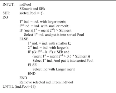
Figure 1.

Pseudocode of LexGA-ML-CFS’ tournament selection.

There are two main differences between the proposed multi-objective LexGA-ML-CFS and the single multi-objective GA-ML-CFS described in [5], which are the way that we evaluate each individual and the way that we select the winner in the tournament selection step. First, in LexGA-ML-CFS, the fitness of an individual is evaluated based on two criteria; (1) the merit function, which is shown in equation (1); and (2) the number of selected features (k). By contrast, GA-ML-CFS evaluates individuals using only the merit function shown in equation (1). Second, LexGA-ML-CFS uses a lexicographic optimization tournament selection, using the merit and k values as highest and lowest priority objective, respectively.

The pseudocode of LexGA-ML-CFS’s tournament selection is shown in Figure 1. When comparing two individuals (feature subsets), if the difference between the merit values of the two individuals is greater than the standard error of the merit (SEmerit) across all individuals in the current population, then the best merit individual is chosen as the tournament’s winner. Otherwise, if the difference of the k value of the individual with larger k (more selected features) minus the k value of the individual with smaller

k (fewer features) is greater than the standard error of k (SEk) across all individuals in the current population and the difference of the merit value of the individual with smaller k minus the merit value of the individual with larger k is larger than half the SEmerit, then the individual with smallest k (smallest feature subset) is chosen. Otherwise, the individual with the largest merit is chosen.

The second condition in the above and statement – i.e., the condition for the difference in merit to be greater than half the SEmerit – was added because, in our preliminary experiments, a lexicographic optimization tournament using only a condition on the difference in k values was leading the GA to select individuals based on the second lexicographic criterion (after a tie being observed in the first criterion) very often, leading the GA to return solutions that had a relatively small number of features but relatively poor predictive accuracy. Hence, the addition of this second condition based on merit, when evaluating the second lexicographic criterion, helps to de-emphasize the importance of

the second lexicographic objective (minimizing the number of selected features), which therefore helps to emphasize the importance of the first lexicographic objective (maximizing predictive accuracy).

6.

Datasets and Experimental Methodology

6.1

Datasets

We used 12 multi-label datasets (shown in Table I), which were obtained from the multi-label dataset repository website (http://mulan.sourceforge.net/datasets.html) [23]. We divided the 12 datasets into two groups: (1) datasets for parameter optimization and (2) datasets for evaluating the multi-label feature selection methods. The parameter optimization group contains the 4 datasets with less than 300 features, while all evaluation datasets have more than 300 features.

TABLE I. DATASET CHARACTERISTICS

Dataset Name

Number of:

Instances Features Labels Avg. Labels per Inst. Parameter Optimization Datasets

CAL500 502 68 174 26.0 Scene 2407 294 6 1.1 Emotions 593 72 6 1.9 Yeast 2417 103 14 4.2 Evaluation Datasets Business 11314 21924 30 1.6 Art 7484 23146 26 1.7 Education 12030 27534 33 1.5 Recreation 12828 30324 22 1.4 Health 9205 30635 32 1.6 Enter.ment 12730 32001 21 1.4 Computer 12444 34096 33 1.5 Science 6428 37187 40 1.5

Note that using a few datasets to optimize parameters for the GAs and evaluating the GAs in the other datasets is not an optimal approach to optimize GA parameters. Intuitively, the predictive performance of the GAs could be improved by doing parameter optimization for each of the 12 datasets separately, using the training set of each dataset. However, we have chosen the former approach mainly for two reasons. First, the GAs have many parameters to be optimized, and it would be very time consuming to optimize parameters separately for each dataset. Hence, we optimize the GA parameters across the three smallest datasets, in terms of both the number of instances and number of features, saving a large amount of computational time. Second, this allows us to try to find GA parameters which are robust across different datasets and can be used as “default” parameters recommended when users do not have time to perform extensive parameter optimization experiments.

Since the datasets in the evaluation group have very large numbers of features (from 21,924 to 37,187 features), before applying the time-consuming multivariate feature selection methods evaluated in this work, a simpler and much faster univariate filter approach was applied in a preliminary stage to all the evaluation datasets. This univariate approach evaluates the quality of each feature separately, ignoring feature interactions, unlike the multivariate methods investigated in this work. The main objective of using this univariate filter approach is to remove all features which have a low correlation with labels before running the multivariate feature selection methods, in order to reduce the search space for such multivariate methods. The multi-label univariate filter method used here simply computes the average correlation between each feature and all class labels, using

INPUT: indPool SEmerit and SEk SET: sorted Pool = {} DO

1st _{ind. = ind. with larger merit;}

2nd _{ind. = ind. with smaller merit;}

IF (merit 1st _{– merit 2}nd_{) > SEmerit}

Select 1st _{ind. and put it into sorted Pool}

ELSE

1st _{ind. = ind. with smaller k;}

2nd _{ind. = ind. with larger k;}

IF ((k 2nd _{– k 1}st_{) > SEk and}

(merit 1st _{– merit 2}nd _{> 0.5 * SEmerit))}

Select 1st _{ind. And put it into sorted Pool}

ELSE

Select ind with Larger merit END

END

Remove selected ind. From indPool UNTIL (ind.Pool={})

equation (2), ranks the features in decreasing order of their equation (2) value, and selects the top n features in the rank. These selected n features are then used as input by the multivariate feature selection methods. We did experiments with four values of

n, namely 100, 200, 300, 400.

6.2

Experimental Setting

There are two main steps in our experimental methodology to use a GA for feature selection: (1) finding the best parameter setting for the GA; and (2) running the GA using the parameter setting obtained from step (1). These steps are described in more detail next.

Step 1: Finding the best parameter setting using parameter optimization datasets. In this step, we find a parameter setting optimized for each of the two GAs (GA-ML-CFS and LexGA-ML-CFS) in order to make a fair comparison between these methods. Note that the Hill Climbing-based ML-CFS does not have any parameters to be optimized.

We considered 6 parameters for the GAs, each with the range of possible values show in Table II. In total, 19 parameter setting combinations were considered (shown in Table III). In the parameter optimization step, the size of GA and LexGA individuals (i.e. the number of features used as input by the GA) is given by the number of features in the dataset used in the experiment; for example, the individual size is equal to 68 and 294 for the CAL500 and Scene datasets, respectively.

TABLE II. RANGE OF POSSIBLE SETTINGS FOR EACH OF 6 PARAMETERS OF THE GA-ML-CFS AND LEXGA-ML-CFS

Parameters Tried Settings

population size (Pop.size) 100, 150, 200, 250 number of generations (Max.Gen) 50, 100, 150, 200 elitism size (Elite) 2, 4, 6, 8 tournament size (Tour.size) 2, 4, 6, 8 crossover probability (Gene.CrossProb) 0.2, 0.3, 0.4, 0.5 mutation probability (Gene.MuteProb) 0.0025,0.005, 0.001, 0.01

TABLE III. PARAMETER SETTINGS FOR THE PARAMETER OPTIMIZATION PROCESS No. Parameters POP Size Max Gen Elite Size Tour Size Gene CrossProb Gene MuteProb PS01 200 100 2 2 0.5 0.01 PS02 100 100 2 2 0.5 0.01 PS03 150 100 2 2 0.5 0.01 PS04 250 100 2 2 0.5 0.01 PS05 200 50 2 2 0.5 0.01 PS06 200 150 2 2 0.5 0.01 PS07 200 200 2 2 0.5 0.01 PS08 200 100 4 2 0.5 0.01 PS09 200 100 6 2 0.5 0.01 PS10 200 100 8 2 0.5 0.01 PS11 200 100 2 4 0.5 0.01 PS12 200 100 2 6 0.5 0.01 PS13 200 100 2 8 0.5 0.01 PS14 200 100 2 2 0.4 0.01 PS15 200 100 2 2 0.3 0.01 PS16 200 100 2 2 0.2 0.01 PS17 200 100 2 2 0.5 0.005 PS18 200 100 2 2 0.5 0.0025 PS19 200 100 2 2 0.5 0.001

Step 2: running the GAs on the evaluation datasets using the parameter setting optimized in the previous step. In this step, we run four types of experiments: (1) running LexGA-ML-CFS using

the parameters optimized in step 1; (2) running GA-ML-CFS using the parameters optimized in step 1; (3) running Hill Climbing-based ML-CFS; and (4) running the Binary Relevance method using kNN. Binary Relevance (BR) is a simple method that transforms the multi-label classification problem into multiple single-label problems – where each problem has a different class label to be predicted, but all problems use the same set of predictive features. Then, the single-label kNN classification algorithm is applied to each problem separately (without any feature selection), and the set of class labels predicted for each test instance is the union of all the class labels predicted by the individual kNN classifiers for that instance [1].

7.

Computational Results

7.1

Computational Results for the Parameter

Optimization Step for the GA and the LexGA

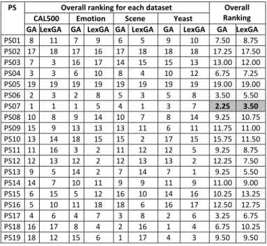
After running GA-ML-CFS and LexGA-ML-CFS using 19 parameter settings on the 4 parameter optimization datasets, the merit (equation (1)) value of the selected feature subset (the best individual returned by the GA) for each parameter setting was calculated. Then we compute the rank of each parameter setting for each dataset based on its merit. That is, the parameter setting with the best merit value for a given GA is given merit rank 1, and the worst parameter setting is assigned rank 19, for each combination of dataset and multi-label predictive accuracy measure (for each of the two GAs separately) – the accuracy measures used are mentioned in the next Section.

TABLE IV. SUMMARY OF RANKING RESULTS FOR PARAMETER SETTING

OPTIMIZATION FOR GA-ML-CFS AND LEXGA-ML-CFS

PS Overall ranking for each dataset Overall 

Ranking

CAL500 Emotion Scene Yeast

GA LexGA GA LexGA GA LexGA GA LexGA GA LexGA

PS01 8 11 7 9 6 5 9 10 7.50 8.75 PS02 17 18 17 16 17 18 18 18 17.25 17.50 PS03 7 3 16 17 14 15 15 13 13.00 12.00 PS04 3 3 6 10 8 4 10 12 6.75 7.25 PS05 19 19 19 19 19 19 19 19 19.00 19.00 PS06 2 3 2 8 5 3 5 8 3.50 5.50 PS07 1 1 1 5 4 1 3 7 2.25 3.50 PS08 10 8 9 14 10 7 8 14 9.25 10.75 PS09 15 9 13 13 13 11 6 11 11.75 11.00 PS10 13 14 18 15 15 2 17 15 15.75 11.50 PS11 11 16 3 2 11 12 12 5 9.25 8.75 PS12 12 13 12 2 12 13 13 2 12.25 7.50 PS13 9 5 14 2 7 14 7 1 9.25 5.50 PS14 14 7 10 11 9 9 11 9 11.00 9.00 PS15 6 15 5 12 16 10 14 16 10.25 13.25 PS16 5 10 11 18 18 6 16 17 12.50 12.75 PS17 4 6 4 7 3 8 2 6 3.25 6.75 PS18 16 17 8 4 2 16 1 4 6.75 10.25 PS19 18 12 15 6 1 17 4 3 9.50 9.50

Next, for each dataset, we produced a ranking of the 19 parameter settings by computing the average of their rank across the accuracy measures. Finally, we produced the overall ranking of the 19 parameter settings by averaging the previously computed rank across all 4 datasets. The results of this ranking procedure are shown in Table IV. These results are averaged over 10 runs with different random seeds. The parameter setting optimized for both the GA and the LexGA is PS07, where population size = 200, number of generations = 200, elitist set size = 2, tournament size =

2, gene crossover probability = 0.5, gene mutation probability = 0.01. These parameter settings are used in all experiments reported in the next Section.

7.2

Experiment Results on Evaluation

Datasets

After running GA-ML-CFS, LexGA-ML-CFS and HC-ML-CFS on the 8 evaluation datasets, the predictive accuracy of the corresponding selected features was evaluated by running the ML-kNN algorithm. Due to the complexity of multi-label classification, no single accuracy measure is enough to capture different aspects of multi-label classification [23,24]. Hence, five different popular measures of multi-label predictive accuracy were used in our experiments: Average Precision (Avg.Pre), which is to be maximized, while Coverage (Cov.), Hamming Loss (H-Loss), One-error (One.Err) and Ranking Loss (R-Loss) are to be minimized. All those measures are discussed in [25].

TABLE V. PREDICTIVE ACCURACIES ON EVALUATION DATASETS

(INDIVIDUAL LENGTH =100)

DT method ML-KNN Classifier

Avg.Pre Cov. H-Loss OneErr R-Loss AR

Busine ss GA 0.873(2) 2.382(1) 0.029(2) 0.127(2) 0.044(2) 1.8 LexGA 0.874(1) 2.391(2) 0.028(1) 0.126(1) 0.044(1) 1.2 HC 0.866(3) 2.418(3) 0.029(3) 0.136(3) 0.044(3) 3.0 BR 0.855(4) 2.726(4) 0.043(4) 0.14(4) 0.049(4) 4.0 Ar t GA 0.529(2) 5.318(2) 0.059(2) 0.588(2) 0.147(3) 2.2 LexGA 0.53(1) 5.32(3) 0.059(1) 0.588(1) 0.147(2) 1.6 HC 0.524(3) 5.307(1) 0.06(3) 0.61(3) 0.134(1) 2.2 BR 0.432(4) 5.971(4) 0.229(4) 0.753(4) 0.177(4) 4.0 E ducation GA 0.542(3) 3.906(2) 0.042(3) 0.608(3) 0.092(2) 2.6 LexGA 0.542(2) 3.914(3) 0.042(2) 0.605(2) 0.093(3) 2.4 HC 0.544(1) 3.872(1) 0.042(1) 0.605(1) 0.092(1) 1.0 BR 0.477(4) 4.645(4) 0.146(4) 0.682(4) 0.11(4) 4.0 Rec reat ion GA 0.535(3) 4.328(3) 0.059(3) 0.604(3) 0.158(2) 2.8 LexGA 0.537(1) 4.295(1) 0.059(1) 0.601(2) 0.157(1) 1.2 HC 0.536(2) 4.327(2) 0.059(2) 0.6(1) 0.158(3) 2.0 BR 0.377(4) 5.604(4) 0.346(4) 0.805(4) 0.222(4) 4.0 He alth GA 0.63(1) 3.799(1) 0.05(1.5) 0.48(3) 0.075(1) 1.5 LexGA 0.629(2) 3.803(2) 0.05(3) 0.48(2) 0.075(3) 2.4 HC 0.629(3) 3.803(3) 0.05(1.5) 0.479(1) 0.075(2) 2.1 BR 0.617(4) 4.062(4) 0.13(4) 0.489(4) 0.079(4) 4.0 En t.men t GA 0.576(3) 3.183(2) 0.057(2) 0.576(3) 0.12(2) 2.4 LexGA 0.577(2) 3.181(1) 0.057(3) 0.575(2) 0.12(1) 1.8 HC 0.579(1) 3.186(3) 0.056(1) 0.57(1) 0.121(3) 1.8 BR 0.466(4) 3.984(4) 0.281(4) 0.715(4) 0.16(4) 4.0 Com pu te r GA 0.621(3) 4.392(3) 0.042(3) 0.455(3) 0.094(3) 3.0 LexGA 0.622(2) 4.388(2) 0.041(2) 0.454(2) 0.094(2) 2.0 HC 0.633(1) 4.2(1) 0.04(1) 0.453(1) 0.09(1) 1.0 BR 0.599(4) 4.84(4) 0.113(4) 0.476(4) 0.102(4) 4.0 Sc ie nce GA 0.447(2) 6.871(2) 0.035(2) 0.699(2) 0.136(2) 2.0 LexGA 0.455(1) 6.837(1) 0.035(1) 0.689(1) 0.135(1) 1.0 HC 0.42(3) 7.462(3) 0.036(3) 0.718(3) 0.151(3) 3.0 BR 0.391(4) 8.113(4) 0.237(4) 0.759(4) 0.165(4) 4.0 Mean GA 2.38 2.00 2.31 2.63 2.13 2.29 LexGA 1.50 1.88 1.75 1.63 1.75 1.70 HC 2.13 2.13 1.94 1.75 2.13 2.01 BR 4.00 4.00 4.00 4.00 4.00 4.00

Tables V-VIII show the predictive performance of the proposed LexGA-ML-CFS and the other methods with different individual lengths – i.e, different number of features pre-selected by the univariate filter method (as explained in Section 6.1), namely 100, 200, 300 and 400 features, respectively. For each method, each table reports the values of each of the five measures of multi-label predictive accuracy mentioned earlier. In Tables V-VIII, LexGA

stands for the LexGA-ML-CFS, GA stands for the single-objective GA-ML-CFS, HC stands for Hill Climbing-based ML-CFS and BR stands for the Binary Relevance method. In these tables, the GA and LexGA results are an average over the results of 5 runs with a different random seed used to create the initial population in each run. The results for HC and BR are based on a single run, since these methods are deterministic.

The numbers between brackets right after the accuracy results denote the ranks achieved by each method – in the range from 1 (best) to 4 (worst). The tables also report, in the last column, the average rank (AR) of each method across all five predictive accuracy measures, for each dataset. The last 4 rows of each table show the mean rank for each method across the 8 datasets, and finally the last column of the last 4 rows shows the average ranks over the 5 predictive accuracy measures and over the 8 datasets.

TABLE VI. PREDICTIVE ACCURACIES ON EVALUATION DATASETS

(INDIVIDUAL LENGTH =200)

DT method ML-KNN Classifier

Avg.Pre Cov. H-Loss OneErr. R-Loss AR

Busine ss GA 0.876(2) 2.291(2) 0.028(2) 0.124(2) 0.041(2) 2.0 LexGA 0.876(1) 2.282(1) 0.028(1) 0.124(1) 0.041(1) 1.0 HC 0.868(3) 2.364(3) 0.029(3) 0.136(3) 0.043(3) 3.0 BR 0.853(4) 2.727(4) 0.043(4) 0.14(4) 0.049(4) 4.0 Ar t GA 0.53(1) 5.301(1) 0.06(2) 0.59(1) 0.147(1) 1.2 LexGA 0.528(2) 5.32(2) 0.06(1) 0.594(2) 0.148(2) 1.8 HC 0.523(3) 5.395(3) 0.06(3) 0.604(3) 0.15(3) 3.0 BR 0.414(4) 7.523(4) 0.558(4) 0.753(4) 0.226(4) 4.0 E ducation GA 0.546(2) 3.912(2) 0.042(2) 0.598(2) 0.093(2) 2.0 LexGA 0.546(3) 3.914(3) 0.042(3) 0.598(3) 0.093(3) 3.0 HC 0.552(1) 3.839(1) 0.042(1) 0.592(1) 0.09(1) 1.0 BR 0.468(4) 5.435(4) 0.272(4) 0.682(4) 0.126(4) 4.0 Rec reat ion GA 0.572(3) 4.143(2) _{LexGA 0.573(2) 4.157(3) 0.055(1) 0.544(1) 0.15(3)} 0.056(3) 0.545(2) 0.15(2) 2.4_2.0 HC 0.573(1) 4.12(1) 0.055(2) 0.545(3) 0.148(1) 1.6 BR 0.314(4) 7.562(4) 0.56(4) 0.804(4) 0.312(4) 4.0 He alth GA 0.681(1) 3.41(1) 0.044(1) 0.405(1) 0.065(1) 1.0 LexGA 0.676(2) 3.43(2) 0.045(2) 0.413(2) 0.065(2) 2.0 HC 0.675(3) 3.444(3) 0.045(3) 0.415(3) 0.065(3) 3.0 BR 0.607(4) 4.038(4) 0.158(4) 0.489(4) 0.082(4) 4.0 En t.men t GA 0.608(1) 3.051(1) 0.055(2) 0.524(1) 0.112(1) 1.2 LexGA 0.604(2) 3.082(2) 0.055(3) 0.532(3) 0.113(2) 2.4 HC 0.602(3) 3.122(3) 0.054(1) 0.53(2) 0.115(3) 2.4 BR 0.451(4) 4.844(4) 0.46(4) 0.715(4) 0.193(4) 4.0 Com pu te r GA 0.637(1) 4.215(1) 0.04(2) 0.437(2) 0.09(1) 1.4 LexGA 0.637(2) 4.224(2) 0.04(3) 0.436(1) 0.091(2) 2.0 HC 0.631(3) 4.28(3) 0.039(1) 0.451(3) 0.091(3) 2.6 BR 0.589(4) 5.1(4) 0.161(4) 0.476(4) 0.111(4) 4.0 Sc ie nce GA 0.465(1) 6.727(1) 0.035(1) 0.668(1) 0.132(1) 1.0 LexGA 0.457(2) 6.83(2) 0.035(2) 0.679(2) 0.135(2) 2.0 HC 0.423(3) 7.402(3) 0.037(3) 0.714(3) 0.15(3) 3.0 BR 0.386(4) 8.877(4) 0.49(4) 0.759(4) 0.183(4) 4.0 Mean GA 1.50 1.38 1.88 1.50 1.38 1.53 LexGA 2.00 2.13 2.00 1.88 2.13 2.03 HC 2.50 2.50 2.13 2.63 2.50 2.45 BR 4.00 4.00 4.00 4.00 4.00 4.00

In general, both GA-ML-CFS and Lex-ML-CFS obtained substantially better predictive accuracy (lower average rank) than the BR approach in every case (individual length = 100, 200, 300 and 400). GA-ML-CFS showed a better average rank (1.53) than LexGA-MLGA-ML-CFS (2.03) and HC-ML-CFS (2.45) when we set the individual length equal to 200 (Table VI), while LexGA-ML-CFS showed a better average rank (1.70) than GA-ML-CFS (2.29) and HC-ML-CFS (2.01) when the individual length was equal to 100 (Table V).

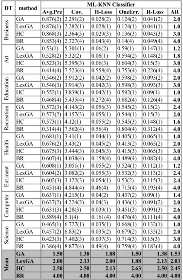
HC-ML-CFS obtains the best results with the two largest individual lengths, i.e. 300 and 400. When the individual length is 300 (Table VII), HC-ML-CFS obtained the best rank of 1.83, versus 1.86 for GA-ML-CFS and 2.31 for LexGA-ML-CFS. In Table VIII, when the individual length is 400, HC-ML-CFS shows the best rank of 1.88, versus 2.18 for GA-ML-CFS and 1.95 for LexGA-ML-CFS.Table IX, third column, compares the average number and percentage of features selected by each method across all datasets for each individual length. The entries for Binary Relevance in this column are “Not applicable” because this method does not perform feature selection. Note that, as the individual length (number of input features) increases, the number of features selected by LexGA-ML-CFS and GA-ML-LexGA-ML-CFS increases much faster than the number selected by HC-ML-CFS. GA-ML-CFS selected the biggest number of features (between 32-37% of individual length), while LexGA-ML-CFS selected a smaller number of features (between 27-31% of the individual length).

TABLE VII. PREDICTIVE ACCURACIES ON EVALUATION DATASETS

(INDIVIDUAL LENGTH =300)

DT method ML-KNN Classifier

Avg.Pre Cov. H-Loss One.Err R-Loss AR

Busine ss GA 0.874(2) 2.315(1) 0.029(2) 0.129(2) 0.041(2.5) 1.9 LexGA 0.874(1) 2.32(2) 0.029(1) 0.126(1) 0.041(2.5) 1.5 HC 0.868(3) 2.372(3) 0.029(3) 0.136(3) 0.041(1) 2.6 BR 0.855(4) 2.736(4) 0.045(4) 0.14(4) 0.049(4) 4.0 Ar t GA 0.528(2) 5.305(2) 0.059(2) 0.595(1) 0.147(2) 1.8 LexGA 0.528(1) 5.28(1) 0.059(1) 0.596(2) 0.146(1) 1.2 HC 0.509(3) 5.487(3) 0.061(3) 0.621(3) 0.154(3) 3.0 BR 0.235(4) 8.568(4) 0.628(4) 0.979(4) 0.27(4) 4.0 E ducation GA 0.551(3) 3.844(2) 0.041(3) 0.592(3) 0.091(3) 2.8 LexGA 0.553(2) 3.851(3) 0.041(2) 0.588(2) 0.091(2) 2.2 HC 0.56(1) 3.766(1) 0.041(1) 0.58(1) 0.089(1) 1.0 BR 0.151(4) 10.153(4) 0.471(4) 0.987(4) 0.284(4) 4.0 Rec reat ion GA _{LexGA 0.579(3) 4.096(3) 0.055(3) 0.538(3) 0.149(3)} 0.583(2) 4.048(2) 0.055(2) 0.537(2) 0.146(2) 2.0_3.0 HC 0.586(1) 3.988(1) 0.055(1) 0.53(1) 0.144(1) 1.0 BR 0.155(4) 9.75(4) 0.674(4) 0.995(4) 0.414(4) 4.0 He alth GA 0.678(2) 3.389(2) 0.044(1) 0.417(2) 0.064(2) 1.8 LexGA 0.677(3) 3.397(3) 0.045(2) 0.42(3) 0.064(3) 2.8 HC 0.682(1) 3.359(1) 0.045(3) 0.415(1) 0.064(1) 1.4 BR 0.602(4) 4.386(4) 0.221(4) 0.489(4) 0.089(4) 4.0 En t.men t GA 0.605(2) 3.053(2) 0.055(2) 0.52(1) 0.112(2) 1.8 LexGA 0.604(3) 3.062(3) 0.056(3) 0.53(3) 0.113(3) 3.0 HC 0.609(1) 3.024(1) 0.054(1) 0.529(2) 0.112(1) 1.2 BR 0.212(4) 7.262(4) 0.514(4) 0.924(4) 0.324(4) 4.0 Com pu te r GA 0.641(2) 4.178(1) 0.039(2) 0.436(1) 0.089(2) 1.6 LexGA 0.638(3) 4.208(3) 0.04(3) 0.439(3) 0.09(3) 3.0 HC 0.641(1) 4.187(2) 0.039(1) 0.438(2) 0.089(1) 1.4 BR 0.252(4) 8.629(4) 0.508(4) 0.939(4) 0.206(4) 4.0 Sc ie nce GA 0.46(1) 6.804(1) 0.035(2) 0.673(1) 0.134(1) 1.2 LexGA 0.453(2) 6.891(2) 0.034(1) 0.681(2) 0.136(2) 1.8 HC 0.422(3) 7.411(3) 0.036(3) 0.715(3) 0.15(3) 3.0 BR 0.119(4) 14.553(4) 0.559(4) 0.967(4) 0.332(4) 4.0 Mean GA 2.00 1.63 2.00 1.63 2.06 1.86 LexGA 2.25 2.50 2.00 2.38 2.44 2.31 HC 1.75 1.88 2.00 2.00 1.50 1.83 BR 4.00 4.00 4.00 4.00 4.00 4.00

The smallest number of selected features was obtained by HC-ML-CFS; this number was between 16-26% of the individual length. Hence, although LexGA-ML-CFS has consistently selected fewer features than GA-ML-CFS, the former still selected more features than HC-ML-CFS, particularly when the size of the feature space is larger.

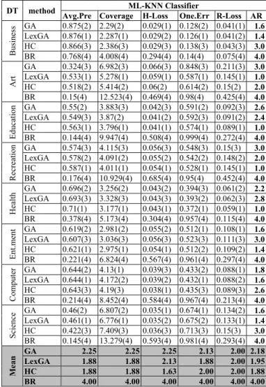
TABLE VIII. PREDICTIVE ACCURACIES ON EVALUATION DATASETS

(INDIVIDUAL LENGTH=400)

DT method ML-KNN Classifier

Avg.Pre Coverage H-Loss One.Err R-Loss AR

Business GA 0.875(2) 2.29(2) 0.029(1) 0.128(2) 0.041(1) 1.6 LexGA 0.876(1) 2.287(1) 0.029(2) 0.126(1) 0.041(2) 1.4 HC 0.866(3) 2.386(3) 0.029(3) 0.138(3) 0.043(3) 3.0 BR 0.768(4) 4.008(4) 0.294(4) 0.14(4) 0.075(4) 4.0 Art GA 0.324(3) 6.982(3) 0.066(3) 0.848(3) 0.211(3) 3.0 LexGA 0.533(1) 5.278(1) 0.059(1) 0.587(1) 0.145(1) 1.0 HC 0.518(2) 5.414(2) 0.06(2) 0.614(2) 0.15(2) 2.0 BR 0.15(4) 12.523(4) 0.469(4) 0.98(4) 0.425(4) 4.0 E ducation GA 0.55(2) 3.883(3) 0.042(3) 0.591(2) 0.092(3) 2.6 LexGA 0.549(3) 3.87(2) 0.041(2) 0.592(3) 0.091(2) 2.4 HC 0.563(1) 3.796(1) 0.041(1) 0.574(1) 0.089(1) 1.0 BR 0.144(4) 9.947(4) 0.508(4) 0.999(4) 0.272(4) 4.0 Recreation GA 0.574(3) 4.115(3) 0.056(3) 0.548(3) 0.15(3) 3.0 LexGA 0.578(2) 4.091(2) 0.055(2) 0.542(2) 0.148(2) 2.0 HC 0.587(1) 4.011(1) 0.054(1) 0.528(1) 0.145(1) 1.0 BR 0.176(4) 10.929(4) 0.685(4) 0.95(4) 0.452(4) 4.0 Health GA 0.696(2) 3.256(2) 0.043(2) 0.394(3) 0.061(2) 2.2 LexGA 0.693(3) 3.328(3) 0.043(3) 0.393(2) 0.062(3) 2.8 HC 0.71(1) 3.177(1) 0.043(1) 0.372(1) 0.059(1) 1.0 BR 0.378(4) 5.173(4) 0.304(4) 0.957(4) 0.115(4) 4.0 En t.men t GA 0.619(2) 2.981(2) 0.055(2) 0.512(1) 0.108(1) 1.6 LexGA 0.607(3) 3.036(3) 0.056(3) 0.523(3) 0.111(3) 3.0 HC 0.621(1) 2.975(1) 0.054(1) 0.512(2) 0.109(2) 1.4 BR 0.221(4) 6.824(4) 0.567(4) 0.961(4) 0.297(4) 4.0 Com puter GA 0.644(2) 4.13(1) 0.039(3) 0.433(2) 0.088(1) 1.8 LexGA 0.644(1) 4.172(2) 0.039(2) 0.432(1) 0.088(2) 1.6 HC 0.643(3) 4.19(3) 0.038(1) 0.435(3) 0.089(3) 2.6 BR 0.214(4) 8.452(4) 0.584(4) 0.967(4) 0.213(4) 4.0 Science GA 0.46(2) 6.807(2) 0.035(1) 0.674(1) 0.134(2) 1.6 LexGA 0.461(1) 6.776(1) 0.035(2) 0.675(2) 0.133(1) 1.4 HC 0.422(3) 7.409(3) 0.036(3) 0.713(3) 0.15(3) 3.0 BR 0.145(4) 13.279(4) 0.593(4) 0.981(4) 0.293(4) 4.0 Mean GA 2.25 2.25 2.25 2.13 2.00 2.18 LexGA 1.88 1.88 2.13 1.88 2.00 1.95 HC 1.88 1.88 1.63 2.00 2.00 1.88 BR 4.00 4.00 4.00 4.00 4.00 4.00

TABLE IX. RESULTS’SUMMARY: AVERAGE NUMBER AND PERCENTAGE

OF SELECTED FEATURES ACROSS 8 DATASETS AND AVERAGE ACCURACY

RANKS ACROSS 8 DATASETS AND 5 PREDICTIVE ACCURACY MEASURES

Individual

Length Method Num. of Selected Features Average predictive accuracy rank

100 GA 36.63 (36.63%) 2.29 LexGA 31.05 (31.05%) 1.70 HC 31.80 (31.80%) 2.01 BR Not applicable 4.00 200 GA 67.80 (33.90%) 1.53 LexGA 54.20 (27.10%) 2.03 HC 46.50 (23.25%) 2.45 BR Not applicable 4.00 300 GA 97.08 (32.36%) 1.86 LexGA 81.18 (27.06%) 2.31 HC 56.40 (18.80%) 1.83 BR Not applicable 4.00 400 GA 130.10 (32.53%) 2.18 LexGA 112.43 (28.11%) 1.95 HC 68.10 (17.03%) 1.88 BR Not applicable 4.00

We used the non-parametric Friedman significance test (based on the methods ranks) to analyse the performance of GA-ML-CFS, LexGA-ML-CFS, HC-ML-CFS and BR. There is a statistically significant difference among these methods as a whole on the evaluation datasets, for each individual length. However, when using

the Hommels post-hoc test to compare the best (control) method against the others, for each individual length, there are no statistically significant differences between the best and the other methods.

8.

Conclusions and Future Research

The results from our experiments show that LexGA-ML-CFS improved predictive accuracy, by comparison with the baseline GA-ML-CFS, HC-ML-CFS and BR methods, when the individual length was set to 100. When the individual length was 200, LexGA-ML-CFS outperformed HC-ML-CFS and BR methods, but it was outperformed by GA-ML-CFS. When the individual length is larger (300 and 400) LexGA-ML-CFS was not able to find a solution (feature subset) better than the solution found by HC-ML-CFS, but LexGA-ML-CFS still found a solution better than the one found by the BR approach. However, overall there was no statistically significant difference between the results of the proposed LexGA-ML-CFS method and other methods.

We also investigated the number of features selected by LexGA-ML-CFS, GA-ML-CFS and HC-ML-CFS. We compared the number of selected features on each dataset across four individual lengths (number of input features). We found that the number of features selected by HC-ML-CFS slowly increases when the individual length is increased from 100 to 200, 300 and 400, while the number of features selected by LexGA-ML-CFS and GA-ML-CFS increases considerably faster when the individual length is increased. Although LexGA-ML-CFS tends to select feature subsets smaller than the ones selected by GA-ML-CFS, the feature subsets selected by LexGA-ML-CFS are still larger than the ones selected by HC-ML-CFS, particularly for larger sizes of the feature space.

One direction for future research is to develop another variation of the fitness function of LexGA-ML-CFS that puts more emphasis on reducing the number of selected features without unduly sacrificing predictive accuracy. Other research directions are to develop new multi-label correlation-based feature selection methods based on other types of search methods such as Beam Search and Ant Colony Optimization.

9.

Acknowledgement

We thank concurrency researchers at Kent for access to the ‘CoSMoS’ cluster, funded by EPSRC grants EP/E049419/1 and EP/E053505/1.

10.

References

[1] G. Tsoumakas, I. Katakis, I. Vlahavas, “Mining Multi-label data,” in Data Mining and Knowledge Discovery Handbook, O. Maimon, L. Rokach, Eds. Springer, Heidelberg, 2010, pp. 667-685.

[2] H. Lui, H. Motoda, Feature Selection for Knowledge Discovery and

Data Mining, Kluwer Academic, Massachusetts, 1998.

[3] A. E. Eiben and J. E. Smith, “Introduction to Evolutionary Computing”, Germany: Springer. 2003

[4] A. A. Freitas, “Evolutionary Algorithms for Data Mining” in O. a. R. L. Maimon, Ed. The Data Mining and Knowledge Discovery Handbook. Berlin: Springer, 2005, pp. 435-467.

[5] S. Jungjit and A.A. Freitas “A New Genetic Algorithm for Multi-Label Correlation-Based Feature Seletion”, in Proceedings ofthe European Symposium on Artificial Neural Networks, Computational Intelligence and Machine Learning (ESANN2015), 22-24 April 2015, in press. [6] M. L. Zhang and Z. H. Zhou, “ML-KNN: a lazy learning approach to

multi-label learning,” Pattern Recognition, 40(7), 2007, pp. 2038-2048. [7] G. Doquire and M. Verleysen, “Feature Selection for Multi-label

Classification Problems,” in Lecture Notes in Computer Science, vol. 6691, Springer, Heidelberg, pp. 9-16, 2011.

[8] G. Doquire and M. Verleysen, “Mutual Information Based Feature Selection for Multi-Label Classification.” Neurocomputing, 122(2013), pp. 148-155, 2013.

[9] W. Chen, J. Yan, B. Zhang, Z. Chen and Q. Yang, “Document transformation for multi-label feature selection in text categorization,”

in Proceeding of IEEE International Conference on Data Mining, 2007,

pp. 451–456.

[10] N. Spolaor, E.A. Cherman and M.C. Monard, “Using ReliefF for Multi-label feature selection,” in Proceedings of Conferencia

Latinoamericana de Informatica, 2011, pp. 960-975.

[11] J. Lee and D. W. Kim, “Feature Selection for Multi-Label Classification using Multivariate Mutual Information.” Pettern recognition Letters,

34(2013), pp. 49-357, 2013.

[12] G. Lastra, O. Luaces, J. R. Quevedo and A. Bahamonde, “Graphical Feature Selection for Multilabel Classification Tasks.” in Proceedings of the 10th international conference on Advances in Intelligent Data

Analysis X. Lecture Notes in Computer Science, vol. 7014, Springer,

Heidelberg, pp. 246-257, 2011.

[13] L. Yu, H. Lui, “Feature Selection for High Dimensional Data: A fast correlation-based feature selection solution,” in Proceeding of the

Twenty International Conference on Machine Learning (ICML-2003),

Washington DC, 2003, pp. 856-863.

[14] M. L. Zhang, J. M. Pena, V. Robles, “Feature selection for multi-label naive Bayes classification.” Information Science, vol. 179(19), pp. 3218-3229, 2009.

[15] Y. Saeys, I. Inza, P. larranaga, “A review of Feature Selection Technique in Bioinformatics.” Bioinformatics, vol. 23(19), pp. 2507-2517, Aug. 2007.

[16] N. Spolaor and G.Tsoumakas, “Evaluating Feature Selection Methods for Multi-Label Text Classification”, BioASQ Workshop, Valencia, Spain, September 27, 2013, 2013.

[17] N. Spolaor, E.A. Cherman, M.C. Monard and H. D. Lee, “Filter Approach Feature Selection Methods to Support Multi-label Learning Based on ReliefF and Information Gain,” in SBIA 2012, Lecture Notes in Artificial Intelligence, vol.7589, L. N. Barros et al, Eds, Springer, Heidelberg, 2012, pp.72-81.

[18] S. Jungjit, A.A. Freitas, M. Michaelis and J. Cinatl, “A Multi-Label Correlation Based Feature Selection Method for the Classification of Neuroblastoma microarray data”, in Advances in Data Mining: 12th Industrial Conference (ICDM 2012): Workshop Proceedings –

Workshop on Data Mining in Life Sciences (DMLS 2012), I.

Bichindaritz, P. Perner, G. Rub, and R. Schmidt, Eds, IBAI Publishing, July 2012, pp. 149-157.

[19] M. A. Hall, “Correlation-based Feature Selection for Discrete and Numeric Class machine Learning,” in Proceedings of the 17th

International Conference on Machine Learning (ICML-2000), Morkan

Kaufmann, San Francisco, 2000, pp.359-366.

[20] S. Jungjit, A.A. Freitas, M. Michaelis and J. Cinatl, “Two Extensions to Multi-Label Correlation-Based Feature Selection: a case study in bioinformatics,” in Proceedings of the 2013 IEEE International Conference on Systems, Man and Cybernetics, Manchester, UK, 2013. [21] S. Jungjit, A.A. Freitas, M. Michaelis and J. Cinatl, “Extending

Multi-Label Feature Selection with KEGG Pathway Information for Microarray Data Analysis,” in Proceedings of the 2014 IEEE International Conference on Computational Intelligence in

Bioinformatics and Computational Biology (CIBCB2014), Hawaii,

USA, 21-25 May 2014.

[22] A.A.Freitas, “A critical review of multi-objective optimization in data mining: a position paper,” ACM SIGKDD Explorations Newsletter 6(2), 77-86, 2004.

[23] G. Tsoumakas, E. Spyromitros-Xioufis, J. Vilcek, I. Vlahavas, “Mulan: A Java Library for Multi-Label Learning”, Journal of Machine Learning Research, 12, 2011 pp. 2411-2414.

[24] E. C. Gonçalves, A. Plastino, and A. A. Freitas. "A Genetic Algorithm for Optimizing the Label Ordering in Multi-label Classifier Chains." In

Tools with Artificial Intelligence (ICTAI), 2013 IEEE 25th International

Conference on, pp. 469-476. IEEE, 2013.

[25] G. Tsoumakas, I. Katakis, I. Vlahavas, “Mining Multi-label data,” in

Data Mining and Knowledge Discovery Handbook, O. Maimon, L.