HAL Id: hal-02354587
https://hal.archives-ouvertes.fr/hal-02354587
Submitted on 7 Nov 2019
HAL
is a multi-disciplinary open access
archive for the deposit and dissemination of
sci-entific research documents, whether they are
pub-lished or not. The documents may come from
teaching and research institutions in France or
abroad, or from public or private research centers.
L’archive ouverte pluridisciplinaire
HAL
, est
destinée au dépôt et à la diffusion de documents
scientifiques de niveau recherche, publiés ou non,
émanant des établissements d’enseignement et de
recherche français ou étrangers, des laboratoires
publics ou privés.
Application of unsupervised nearest-neighbor
density-based approaches to sequential dimensionality
reduction and clustering of hyperspectral images
Claude Cariou, Kacem Chehdi
To cite this version:
Claude Cariou, Kacem Chehdi.
Application of unsupervised nearest-neighbor density-based
ap-proaches to sequential dimensionality reduction and clustering of hyperspectral images. Image and
Signal Processing for Remote Sensing, Sep 2018, Berlin, Germany. pp.16, �10.1117/12.2325530�.
�hal-02354587�
Application of unsupervised nearest-neighbor density-based
approaches to sequential dimensionality reduction and
clustering of hyperspectral images
Claude Cariou and Kacem Chehdi
Univ Rennes / Enssat
SHINE/TSI2M team
Institute of Electronics and Telecommunications of Rennes (IETR) - UMR CNRS 6164
6, rue de Kerampont, 22300 Lannion, France
ABSTRACT
In this communication, we address the problem of unsupervised dimensionality reduction (DR) for hyperspectral images (HSIs), using nearest-neighbor density-based (NN-DB) approaches. Dimensionality reduction is an im-portant tool in the HSI processing chain, aimed at reducing the high redundancy among the HSI spectral bands, while preserving the maximum amount of relevant information for further processing. Basically, the idea is to formalize DR as the process of partitioning the spectral bands into coherent band sets. Two DR schemes can be set up directly, one based on band selection, and the other one based on band averaging. Another scheme is proposed here, based on compact band averaging. Experiments are conducted with hyperspectral images
composed of an AISA Eagle HSI issued from our acquisition platform, and the AVIRISSalinas HSI. We evaluate
the efficiency of the reduced HSIs for final classification results under the three schemes, and compare them to
the classification results without reduction. We show that despite a high dimensionality reduction (<8% of the
bands left), the clustering results provided by NN-DB methods remain comparable to the ones obtained without DR, especially for GWENN in the band averaging case. We also compare the classification results obtained after applying other unsupervised or semi-supervised DR schemes, based either on band selection or band averaging, and show the superiority of the proposed DR scheme.
Keywords: Dimensionality reduction, clustering, hyperspectral image, nearest neighbor, density estimation.
1. INTRODUCTION
Dimensionality reduction (DR) is an important tool in the hyperspectral image (HSI) processing chain. Indeed, DR is aimed at reducing the high redundancy which can be observed between spectral bands, and therefore can be useful to eliminate the most redundant bands while preserving the most informative ones. DR is highly desirable since it summarizes the informational content with minimum impact on the further processing tasks such as pixel classification, therefore allowing a considerable gain in data storage and processing.
In this communication, we address the problem of unsupervised DR for HSIs, using nearest-neighbor density-based (NN-DB) approaches. NN-DB methods are initially automatic classification methods designed to partition data objects without specifying neither the number of clusters to be found nor learning samples. In this sense they are different from the state of the art K-Means and FCM clustering methods. Moreover, they are deter-ministic, very simple to implement, and some of them are non iterative. Among the NN-DB approaches one can
cite ModeSeek,1 knnDPC,2, 3 knnClust,4 and GWENN-WM (Graph WatershEd using Nearest Neighbors with
Weighted Mode).2, 5
The present work studies the applicability of NN-DB methods to DR, which is seen as a processing task previous to clustering. More precisely, considering the fact that NN-DB methods (like other clustering methods) automatically provide exemplar objects which are representative of the clusters, and due to its good performances
Further author information:
in clustering, we investigate the potential of GWENN and other NN-DB methods to reduce the dimensionality of HSIs by performing band clustering in an unsupervised manner.
The paper is organized as follows: in Section 2, we provide an overview of related works in the field of dimensionality reduction focusing on HSIs, and point out the need for unsupervised approaches which do not constraint the user to specify the number of retained bands; in Section 3, we detail the implementation of NN-DB methods in the HSI processing chain, and provide improvements of the baseline selection of band exemplars; Section 4 describes an experimental study of the proposed scheme, involving two HSIs, namely an AISA Eagle HSI acquired by our hyperspectral platform in the framework of a study on seashore algae habitats, and the
AVIRISSalinas HSI; we conclude in Section 5.
2. RELATION TO PREVIOUS WORKS AND MOTIVATION
In a recent work,2 a set of nearest-neighbor density-based clustering methods was proposed and compared in
the context of large scale hyperspectral image pixel partitioning. The conclusions of this work were that NN-DB methods are interesting alternatives to a classical (semi-supervised) clustering methods such as fuzzy c-means (FCM), providing results which are faster, more efficient in terms of classification accuracy, and deterministic. These methods only rely on the computation of a nearest neighbor (NN) graph from the original data set,
obtained by a greedy NN search procedure. This graph is governed by a single parameterk, i.e. the number of
nearest neighbors (NNs) which is set by the used. Also, a model of local (point-wise) density is adopted in Ref.
2, still depending on the same parameterk:
ρ(xm)∝
k
P
xj∈kNN(xm)d(xm,xj)
, 1≤m≤N, (1)
whereN is the number of objects, andkNN(xm) is the set of nearest neighbors toxmaccording to the Euclidean
distanced(., .). Using thekNN graph and the density model above, the four NN-DB methods described in Ref.
2, represent different partitioning strategies by aggregation of objects based on the interaction between NNs’ local densities. These approaches have two important features: the first one is that they do not require the explicit knowledge of the number of clusters which form the partition, and the second one is the stability of the
number of clusters with respect tokaround the optimal working point. Similar examples of adaptation of initial
clustering methods to HSI DR have been proposed in the literature. For example a refinement of the the K-Means
algorithm has been shown to provide superior classification accuracy than similar band reduction methods.6 In
this case the extracted bands are chosen as the centers of the band clusters. However, this approach is still semi-supervised since it requires the user to specify the number of bands to retain. Actually, few unsupervised methods derived from clustering exist which automatically outputs some optimal number of bands. Of course the classical principal component analysis (PCA) is able to provide a reduced representation of the original data by projecting it onto subspaces with greater projected data variances. But, in its baseline implementation, PCA implies that the extracted bands are linear combinations of the original bands, not necessarily accounting for their relative spectral position and adjacency. One interesting implementation of band selection by clustering
was proposed in Qian et al.7 Their method is based on Affinity Propagation (AP),8 which requires no critical
parameter to work and is able to provide an optimal number of clusters by maximizing a criterion involving the
sum of ’responsibilities’ and ’availabilities’. In the context of HSI DR, AP produces a set of so-calledexemplar
bands which are the most representative of the whole band set. In essence, the exemplar bands play the same
role as the centers of the band clusters in Ref. 6. More recently, following the work of Rodriguez and Laio9
on density-based clustering, Tang et al.10 proposed a method, called FDPC (Fast Density Peak Clustering) for
unsupervised band selection. The two latter methods were found to be more efficient in terms of classification
accuracy than other band selection techniques, including Information Divergence (ID)11 and Maximum Variance
PCA (MVPCA).12
The unsupervised band selection methods cited above provide, via the band exemplars, an optimal subset of individual bands which best represent the subbands formed owing to the clustering procedure. An alternative
way is to summarize the spectral information by averaging the bands found in each subband. Averaging has
two positive effects: (i) the whole spectral content is accounted for; (ii) one might expect noise reduction. In
proposition of an unsupervised mutual-information based called BandClust,13 which automatically provides an
optimal number of bands from averaged neighboring bands.
The motivation behind the present work is to evaluate the reliability of NN-DB methods (especially GWENN) when used to cluster spectral bands (instead of objects) efficiently, and to compare this approach with similar DR methods. Another indirect objective is to evaluate the difference in DR relevance between band selection (as directly offered by band exemplars) and band averaging (as an alternative way to summarize the spectral information).
3. NN-DB DIMENSIONALITY REDUCTION BY BAND CLUSTERING
In this section we detail the different approaches proposed to perform DR on HSIs based on NN-DB band clustering. The first one is a band selection method based on band exemplars issued from the clustering procedure; the second one relies on band averaging using the band clusters outputted; the third one introduces a constraint to insure the spectral compactness of the retained bands, before averaging.
3.1 Exemplar band selection
Let a hyperspectral image be rearranged (thanks to image row or column stacking) as a collection
X = {xi= [xi(1), . . . , xi(N)]}i=1,...,B of N-dimensional vectors, where N is the number of pixels in the HSI,
and B is the original number of spectral bands (or features). It is important to notice here that, despite the
potentially high number of spectral bandsB, we still assumeB ≪N, so that the dimensionality of the vectors
is very high.
The principle of band clustering consists in grouping the spectral bands {xi}i=1,...,B into coherent clusters,
without much prior information. NN-DB approaches to band clustering are based upon the availability of
a k-nearest neighbor (kNN) graph, i.e. for each spectral band the set of the k closest bands (w.r.t. some
distance metric), ordered by ascending distance. The choice of the metric can be of importance due to the high dimensionality of the representation space. However, we have not further investigated this issue, and simply
used the Euclidean distanced(xi,xj) =kxi−xjk2 throughout this work.
The implementation of NN-DB methods to HSI DR is rather straightforward, and basically consists of applying
the clustering method to the transposed array of original data: each bandxi is an object (rather than a feature),
and must belong to one and only one band cluster. NN-DB methods also require to compute a local density for each band from its neighboring bands. In the present work, we propose to replace the density model stated in Eq. 1 by the following one:
ρ(xm)∝
X
xj∈kNN(xm)
d−1(x
m,xj) , 1≤m≤B. (2)
This choice appears to provide better results than the one in Eq. 1 in terms of classification accuracy and therefore has been retained in our experiments.
NN-DB methods were described in Ref. 2, with four methods compared: ModeSeek, knnDPC, knnClust-WM, and GWENN-WM. Due to space limitation, we provide only the DR version of GWENN-WM in Algorithm 1. Contrarily to the three other ones, this algorithm is non iterative and therefore has fully controlled complexity.
wmodeis a function computing the class label of the current bandmbased on the labels of its nearest neighbors
(inRN) as well as their respective densities. Note that an additional loop traversing the spectral bands has been
added w.r.t. Ref. 2, which helps stabilizing the formed clusters by merging isolated bands into existing band clusters. The band exemplars issued from the algorithm are expected to be the most representative of the whole HSI.
Algorithm 1GWENN-WM-DR
Require:
X={xm},xm∈RN, m= 1, . . . , B; % The set of spectral bands to cluster
k, the number of NNs;
Ensure: The vector of bands’ labelsc= [c1, . . . , cB] t
; the set of band exemplarsE;
1) ComputeD, theB×karray of distances (in ascending order) between each band and its kNNs.
2) ComputeJ={jm}m=1,...,B,jm=
j1
m, jm2, . . . , jmk
, theB×karray of indices of each object’skNNs.
3) Compute the pointwise densities{ρ(m)}m=1,...,B following Eq. (2).
4) Computeρ′=DescendSort(ρ), keepkNNs indicesi= [i1, i2, . . . , iM]t:ρ′=
ρ(i).
5)N C = 1; %N C is the current number of band clusters
ci1 =N C; % The ”denser” band takes the first label
E={i1}; % The set of band exemplars is initialized with the index of the denser band
P =∅;
form= 2 :B do % First, main pass
P ←P∪im−1; Q=P∩jim; if Q6=∅ then cim =wmode(cQ,ρQ); else N C =N C+ 1; cim =N C;
E ← E ∪ {im}; % Add imto the set of band exemplars
end if end for c′
=c;
form= 1 :B do % Second, refinement pass
Q=jm; c′ m=wmode(cQ,ρQ); end for c=c′;
3.2 Band averaging
In the above scheme, DR is performed by simple band selection based on the band exemplars found by NN-DB
methods. Following Vermillion et al.,14 narrow bands are not necessarily the best choice, and larger bandwidths
can increase the signal to noise ratio. Band averaging has been promoted in Belluco et al.15 as an effective
feature reduction method. In Ref 13, band averaging has been shown to provide superior results compared to some semi-supervised band selection methods.
Therefore, in the present work, since NN-DB methods (like other band clustering methods) end up with coherent groups of bands, the natural way to perform band averaging is to compute the mean of the bands
within each formed cluster, i.e. of the bands having identical labelcl,1≤l≤N C, whereN C is the number of
band clusters.
3.3 Band averaging with compactness constraint
As such, band clustering does not guarantee that the band partitions only contain spectrally neighboring bands, i.e. bands which are spectrally adjacent. This is why it can be useful to modify the NN-DB methods to avoid merging spectrally distant bands into the same band cluster, therefore preserving the physical nature of hyperspectral image formation.
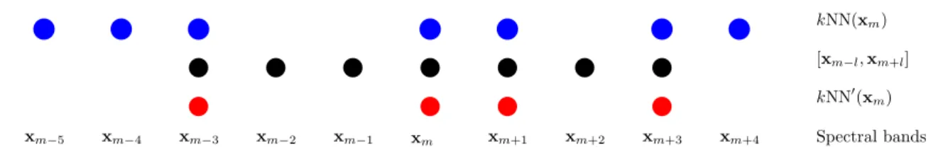
To tackle this problem, we propose here a simple approach which can avoid the above problem. The idea is to
modify the k-NN graph such as to exclude, from the nearest neighbor bands of one specific band, those which
given bandxm is modified: consider the (compact) set of contiguous spectral bands [xm−l,xm+l] (black dots),
andkNN(xm) the set of NN bands found by the NN search (blue dots). Then the NN-DB methods will use as
the modified NNs the set intersection of the latter, i.e.:
kNN′
(xm) = [xm−l,xm+l]∩kNN(xm) , 1≤m≤B. (3)
Since|kNN′
| ≤ |kNN| the computation of the density in Eq. (2) is adjusted in consequence. This constrained NN band clustering scheme insures that the band clusters created by the NN-DB methods are compact on the ordered set of spectral bands. One disadvantage of this approach is that it requires an additional parameter,
l, governing the ’spectral scope’ around the current band. We found in our experiments that takingl=k is a
fairly efficient choice, thereby reducing the parametrization to the sole value ofk.
b b b b b b b xm xm+1 xm+2 xm+3 xm−1 xm−2 xm−3 b b b b b xm−4 xm−5 xm+4 Spectral bands kNN(xm) kNN′ (xm) [xm−l,xm+l] b b b b b b
Figure 1. Illustration of constrained NN band subsetting prior to NN-DB HSI DR (k= 7, l= 3).
In the following, the DR versions of GWENN-WM will be named GWENN-DR.
4. EXPERIMENTAL STUDY
4.1 Experiment 1:
Salinas
HSI
In this experiment, we analyzed the potential use of one NN-DB method, namely GWENN-DR (with weighted mode) to perform efficient band reduction on a popular (and well conditioned) benchmark image. To this end, we
selected theSalinas HSI∗. This image was acquired by the AVIRIS sensor in 1998 over agricultural fields. It has
a spatial size of 512×217 pixels, and 204 spectral bands. The reference map is composed of 16 vegetation classes
as shown on Figure 2. This map was used for assessing the clustering results in terms of classification accuracy, following the procedure described in Ref. 16 to best align unsupervised classification results with ground truth data. After careful examination of the spectral signatures in this HSI, we found that four pixels were spectrally
altered by some unknown effect (at spatial locations (131,132),(131,133),(500,51) and (500,52)), and thus we
have rejected them as outliers.
The experiment was designed to compare GWENN-DR methods with other band clustering methods as well as other state of the art DR methods. For each method, the HSI is first processed for DR; then the reduced HSI undergoes an unsupervised clustering step; finally the clustering result is evaluated owing to the reference map. The choice of the clustering method to be applied after DR was guided by the willing to keep the processing chain as much unsupervised as possible. This is why we have also selected NN-DB clustering methods (and more
particularly GWENN) due to their interesting performances.2 Note that in this experiment, and differently to
our previous works, we did not use here any multiresolution analysis scheme to accelerate the clustering stage.
Instead, a fullkNN graph (with k≤3000, i.e. less than 3% of the number of objects) was computed over the
whole HSI (111104 objects).
4.1.1 Dimensionality reduction
Before applying the DR stage, each spectral band of the originalSalinas HSI was normalized to zero mean and
unit variance. This step was found to provide better results in terms of classification accuracy at the end of the processing chain, w.r.t. no normalization (i.e. original data).
We first applied GWENN-DR to the normalized HSI. For this, we usedk= 5 in Algorithm 1, which provided 15
band clusters. At this point, two DR results can be produced, i.e. a band selection (BSel) result based on the
band exemplars found by GWENN-DR, and a band averaging (BAvg) result based on the means of each band
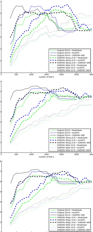
cluster, each result consisting of 15 bands. Then we applied three NN-DB methods, namely ModeSeek, knnDPC and GWENN-WM to both reduced images as well as to the original HSI (204 bands). Figure 3 displays three classification performance indices, namely the Average Correct Classication Rate (ACCR), the Overall Correct
Classication Rate (OCCR), and the kappa index of agreement as a function of the number of NNs k used in
the NN-DB clustering stage. These curves appeal several comments. Firstly, it can be observed a differentiated
behavior in average performance indices between BSel and BAvg, on both the quality of the clustering result
(higher forBAvg) and on the number of NNs required to reach the optimum clustering (higher forBSel). Hence
in average, it appears at least experimentally that band averaging should be preferred to band selection whatever the NN-DB used. Secondly, ModeSeek seems less efficient than knnDPC or GWENN-WM in average on the DR image, and this is also true for the original HSI. Lastly, one can see that knnDPC and GWENN-WM are able to provide classification performance indices which can locally fairly compare with the ones obtained from the original HSI; for instance, the OCCR and kappa indices of GWENN-WM applied to GWENN-DR image
afterBAvg are less than 2.8% lower than the maximum ones obtained by applying GWENN-WM on the original
HSI. Therefore one can conclude that GWENN-DR with band averaging is appropriate for HSI dimensionality reduction.
4.1.2 Comparison with other DR methods
Here, we selected GWENN-WM as the only classifier, whereas we applied to it the results of several DR methods.
These include a semi-supervised band selection method (LP/OSP17) where the number of selected bands is
specified by the user, an unsupervised band averaging based on AP,7, 8 and an unsupervised band averaging
method (BandClust13). We also included the results issued from the third band grouping strategy discussed in
3.3, which we calledCBAvg, standing for compact band averaging.
In order to verify and compare the spectral coherence of the band clustering schemes, we show in Figure 4 the location of the band clusters, exemplars or selection subsets given by the above methods. For GWENN-DR, one
can see that, except for the lowest and highest bands, most band exemplars found by GWENN-BSelare located
near the center of their corresponding band cluster in GWENN-BAvg. However, some of the band clusters
formed for the latter are non compact, especially between bands 40 and 80. As expected, the situation is better
for GWENN-CBAvg, for which the band clusters are strictly compact over the spectral range. BandClust also
provides compact sub-bands (this is normal since it is a band splitting algorithm) which slightly differ from
the previous ones. Specifically, the red edge18 (bands 34-41) is clearly identified as a cluster, whereas only the
inflection point of the red edge is marked as a singleton cluster by GWENN-CBAvg. However, the number of
sub-bands found automatically by BandClust (14) is very close to the one obtained with the GWENN-DR approaches.
Comparatively, the LP/OSP and the AP-BAvg methods exhibit lesser coherence in the band selection or band
clusters outputted.
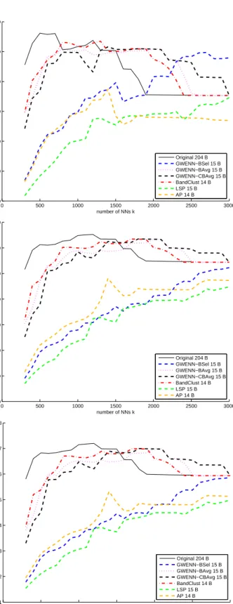
Figure 5 displays the classification performance indices as above, where the previous curves of GWENN-DR with
BSelandBAvg are reported again together with the other studied methods. Among the DR methods,
GWENN-CBAvgachieves superior clustering performances and stability than GWENN-BAvg and BandClust fork≥1800
(highest OCCR: 73.52% atk = 1800). The BandClust DR result provides overall efficient clustering. Besides,
LP/OSP (BSel) is inferior to GWENN-BSelfor all values ofkin the clustering stage. Finally, AP provides poor
results, despite it is here a band averaging method. For the two latter methods, these results are in agreement with the previous observations regarding the location of the band clusters and selection subsets.
4.2 Experiment 2: Classification of foreshore algae species
We present here an application of the proposed DR to a larger HSI. Similarly as above, DR is followed by unsupervised clustering using GWENN-WM with the density estimation proposed in Eq. (2). The difference here relies in the way we manage the size of the HSI; for this we used the multiresolution scheme proposed in Ref. 2.
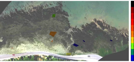
The HSI has been acquired on June 13, 2014 by our hyperspectral imager (AISA Eagle) mounted on an aircraft over the region near the city of Veulettes-sur-Mer, Normandy, France. The objective of the aerial survey was the
identification of algae species and substrates. A number of regions were identified at the ground level as relatively homogeneous (despite the high complexity of the foreshore coverage), which were reported to produce a ground truth (GT) map with ten classes (6608 pixels). Figure 6 displays a RGB view of the HSI with superimposed GT
map. The size of the image cube is (1264×592) pixels×126 bands.
In this experiment, we selected for comparison two NN-DB DR methods, i.e. GWENN-BAvg and
GWENN-CBAvg, as well as BandClust and AP-DR. The reduced HSIs, as well as the original (full bands) HSI then
entered the same clustering procedure, i.e. GWENN-WM, with varying number of NNskas above, and a 4-level
resolution. The advantage of using GWENN-WM is its capability to stabilize the number of exemplars from one
scale resolution to the others.2 As above, ACCR, OCCR and kappa indices were calculated for evaluation.
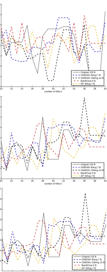
Figure 8 shows the comparison of clustering performance indices for k in the range [20,40]. Due to the
complexity of the foreshore environment, with numerous mixtures of substrates, algae species and presence of water in more or less large puddles, it is not surprising that the classification indices are lower in average than
in the previous experiment. However, it can be seen that GWENN-CBAvg is able to reach the highest OCCR
and kappa indices among the other DR methods, fork= 36. We show in Figure 7 the corresponding clustering
result. Twelve different classes have been found among the pixels of the ground truth, whereas the total number of clusters is 19. One important point in this experiment is the observation that DR is able to provide a reduced band set which is more relevant for further clustering than the original HSI with 126 bands.
5. CONCLUSION
In this paper, we have proposed the use of nearest-neighbor density-based clustering approaches to spectral band grouping in the context of dimensionality reduction (DR) for hyperspectral images. More precisely, we have investigated three DR strategies, i.e. band selection based on band cluster exemplars directly issued from the band clustering procedure, then the averaging of bands belonging to each cluster, and finally a constrained band averaging scheme aiming to preserve the spectral compactness within each form band cluster. Experiments with a popular benchmark HSI and on a HSI acquired by our AISA Eagle hyperspectral acquisition platform allow us to conclude on the effectiveness of NN-DB clustering-based DR with respect to other unsupervised or semi-supervised methods like LP/OSP and AP. Beyond these observations, the experimental results in the present work also confirm the superiority of the band averaging principle to summarize the spectral information, with respect to simple band selection.
REFERENCES
[1] Duin, R. P. W., Fred, A. L. N., Loog, M., and Pekalska, E., “Mode Seeking Clustering by KNN and Mean
Shift Evaluated.,” in [Proc. Structural and Syntactic Patt. Rec. and Stat.Tech. in Patt. Rec.], Gimel’farb,
G. L., Hancock, E. R., Imiya, A., Kuijper, A., Kudo, M., Omachi, S., Windeatt, T., and Yamada, K., eds.,
Lecture Notes in Computer Science7626, 51–59, Springer, Hiroshima, Japan (2012).
[2] Cariou, C. and Chehdi, K., “Nearest neighbor-density-based clustering methods for large hyperspectral
images,” in [Proceedings of SPIE - The International Society for Optical Engineering], 10427(2017).
[3] Du, M., Ding, S., and Jia, H., “Study on density peaks clustering based on k-nearest neighbors and principal
component analysis,”Knowledge-Based Systems99, 135–145 (2016).
[4] Tran, T. N., Wehrens, R., and Buydens, L. M. C., “KNN-kernel density-based clustering for high-dimensional
multivariate data,”Computational Statistics & Data Analysis51(2), 513–525 (2006).
[5] Cariou, C. and Chehdi, K., “A new k-nearest neighbor density-based clustering method and its application
to hyperspectral images,” in [IEEE Intern. Geoscience and Remote Sensing Symposium], 6161–6164 (2016).
[6] Su, H., Yang, H., Du, Q., and Sheng, Y., “Semisupervised band clustering for dimensionality reduction of
hyperspectral imagery,”IEEE Geoscience and Remote Sensing Letters8(6), 1135–1139 (2011).
[7] Qian, Y., Yao, F., and Jia, S., “Band Selection for Hyperspectral Imagery Using Affinity Propagation,”IET
Computer Vision3(4), 213–222 (2009).
[8] Frey, B. J. and Dueck, D., “Clustering by Passing Messages Between Data Points,” Science 315(5814),
972–976 (2007).
[9] Rodriguez, A. and Laio, A., “Clustering by fast search and find of density peaks,” Science 344(6191),
[10] Tang, G., Jia, S., and Li, J., “An enhanced density peak-based clustering approach for hyperspectral band
selection,” in [2015 IEEE International Geoscience and Remote Sensing Symposium (IGARSS)], 1116–1119
(July 2015).
[11] Chang, C. I. and Wang, S., “Constrained band selection for hyperspectral imagery,”IEEE Transactions on
Geoscience and Remote Sensing 44(6), 1575–1585 (2006).
[12] Chang, C.-i., Member, S., Du, Q., and Member, S., “A Joint Band Prioritization and Band- Decorrelation
Approach to Band Selection for Hyperspectral Image Classification,”IEEE Transactions on Geoscience and
Remote Sensing37(6), 2631–2641 (1999).
[13] Cariou, C., Chehdi, K., and Le Moan, S., “BandClust: An unsupervised band reduction method for
hyper-spectral remote sensing,” IEEE Geoscience and Remote Sensing Letters8(3), 565–569 (2011).
[14] Vermillion, Stephanie C.; Raque˜no , Rolando; Simmons, R., “Spectral band characterization for
hyper-spectral monitoring of water quality,” in [Proceedings of the Tenth JPL Airborne Earth Science Workshop],
435–443 (2001).
[15] Belluco, E., Camuffo, M., Ferrari, S., Modenese, L., Silvestri, S., Marani, A., and Marani, M., “Mapping
salt-marsh vegetation by multispectral and hyperspectral remote sensing,” Remote Sensing of
Environ-ment105(1), 54–67 (2006).
[16] Cariou, C. and Chehdi, K., “Unsupervised nearest neighbors clustering with application to hyperspectral
Images,”IEEE Journal on Selected Topics in Signal Processing9(6), 1105–1116 (2015).
[17] Du, Q. and Yang, H., “Similarity-based unsupervised band selection for hyperspectral image analysis,”
IEEE Geoscience and Remote Sensing Letters5(4), 564–568 (2008).
[18] Smith, K. L., Steven, M. D., and Colls, J. J., “Use of hyperspectral derivative ratios in the red-edge region
(a) (b)
Figure 2.Salinas HSI. (a): Color composite (bands 30, 20, 10); (b): Reference map. 0 500 1000 1500 2000 2500 3000 20 30 40 50 60 70 80 number of NNs k ACCR (%) Original 204 B + ModeSeek Original 204 B + knnDPC Original 204 B + GWENN−WM GWENN−BAvg 15 B + ModeSeek GWENN−BAvg 15 B + knnDPC GWENN−BAvg 15 B + GWENN−WM GWENN−BSel 15 B + ModeSeek GWENN−BSel 15 B + knnDPC GWENN−BSel 15 B + GWENN−WM 0 500 1000 1500 2000 2500 3000 10 20 30 40 50 60 70 80 number of NNs k OCCR (%) Original 204 B + ModeSeek Original 204 B + knnDPC Original 204 B + GWENN−WM GWENN−BAvg 15 B + ModeSeek GWENN−BAvg 15 B + knnDPC GWENN−BAvg 15 B + GWENN−WM GWENN−BSel 15 B + ModeSeek GWENN−BSel 15 B + knnDPC GWENN−BSel 15 B + GWENN−WM 0 500 1000 1500 2000 2500 3000 0.1 0.2 0.3 0.4 0.5 0.6 0.7 0.8 number of NNs k kappa Original 204 B + ModeSeek Original 204 B + knnDPC Original 204 B + GWENN−WM GWENN−BAgv 15 B + ModeSeek GWENN−BAgv 15 B + knnDPC GWENN−BAgv 15 B + GWENN−WM GWENN−BSel 15 B + ModeSeek GWENN−BSel 15 B + knnDPC GWENN−BSel 15 B + GWENN−WM
Figure 3. Salinas HSI: Comparison of NN-DB classifica-tion results (ModeSeek, knnDPC and GWENN-WM) with-out DR, and after applying GWENN-DR in band selection (BSel) vs. band averaging (BAvg). Top: Average correct classification rate (ACCR); middle: Overall correct classifi-cation rate (OCCR); bottom: kappa index.
Band number 20 40 60 80 100 120 140 160 180 200 GWENN−BSel GWENN−BAvg GWENN−CBAvg BandClust LP/OSP AP−BAvg
Figure 4.SalinasHSI: Comparison of band selection or band groups obtained with different DR methods. Each color corresponds to a particular band exemplar or band group.
0 500 1000 1500 2000 2500 3000 20 30 40 50 60 70 80 number of NNs k ACCR (%) Original 204 B GWENN−BSel 15 B GWENN−BAvg 15 B GWENN−CBAvg 15 B BandClust 14 B LSP 15 B AP 14 B 0 500 1000 1500 2000 2500 3000 10 20 30 40 50 60 70 80 number of NNs k OCCR (%) Original 204 B GWENN−BSel 15 B GWENN−BAvg 15 B GWENN−CBAvg 15 B BandClust 14 B LSP 15 B AP 14 B 0 500 1000 1500 2000 2500 3000 0.1 0.2 0.3 0.4 0.5 0.6 0.7 0.8 number of NNs k kappa Original 204 B GWENN−BSel 15 B GWENN−BAvg 15 B GWENN−CBAvg 15 B BandClust 14 B LSP 15 B AP 14 B
Figure 5. Salinas HSI: Comparison of GWENN-WM clas-sification results after applying several DR methods. Top: Average correct classification rate (ACCR); middle: Overall correct classification rate (OCCR); bottom: Kappa index.
Fucus > 90% Ulva 80% Ulva on sandy rock Enteromorpha on silted rock Limestone w/ < 20% algae in large puddles Calcareous rock w/ <20% algae Rock w/ <10% algae Rock w/ >10% algae Small pebbles Large pebbles
Figure 6. AISA Eagle HSI (Color composite, bands 57, 36, 14) and superimposed ground truth map.
Figure 7. Best clustering result among the selected unsupervised methods, in terms of OCCR and kappa index, and obtained after DR with GWENN-CBAvg.
20 22 24 26 28 30 32 34 36 38 40 30 35 40 45 50 55 60 65 70 number of NNs k ACCR (%) Original 126 B GWENN−BAvg 7 B GWENN−CBAvg 10 B BandClust 6 B AP−BAvg 7 B 20 22 24 26 28 30 32 34 36 38 40 35 40 45 50 55 60 65 70 75 number of NNs k OCCR (%) Original 126 B GWENN−BAvg 7 B GWENN−CBAvg 10 B BandClust 6 B AP−BAvg 7 B 20 22 24 26 28 30 32 34 36 38 40 0.35 0.4 0.45 0.5 0.55 0.6 0.65 0.7 number of NNs k kappa Original 126 B GWENN−BAvg 7 B GWENN−CBAvg 10 B BandClust 6 B AP−BAvg 7 B
Figure 8.AISA Eagle HSI: Comparison of GWENN-WM classification results after applying several DR methods. Top: Average correct classification rate (ACCR); middle: Overall correct classification rate (OCCR); bottom: Kappa index.