Automatic Modulation Classification Using Cyclic Features via Compressed Sensing

Rochester Institute of Technology

RIT Scholar Works

Theses

12-14-2018

Automatic Modulation Classification Using Cyclic

Features via Compressed Sensing

Andrew J. Ramsey

Follow this and additional works at:https://scholarworks.rit.edu/theses

This Thesis is brought to you for free and open access by RIT Scholar Works. It has been accepted for inclusion in Theses by an authorized administrator of RIT Scholar Works. For more information, please [email protected].

Recommended Citation

Ramsey, Andrew J., "Automatic Modulation Classification Using Cyclic Features via Compressed Sensing" (2018). Thesis. Rochester Institute of Technology. Accessed from

Automatic Modulation Classification Using Cyclic

Features via Compressed Sensing

Automatic Modulation Classification Using Cyclic

Features via Compressed Sensing

Andrew J. Ramsey December 14, 2018

A Thesis Submitted in Partial Fulfillment of the Requirements for the Degree of Master of Science

in Computer Engineering

Automatic Modulation Classification Using Cyclic

Features via Compressed Sensing

Andrew J. Ramsey

Committee Approval:

Dr. Andrés KwasinskiAdvisor Date

Department of Computer Engineering

Dr. Marcin Łukowiak Date

Department of Computer Engineering

Dr. Panos Markopoulos Date

Abstract

Cognitive Radios (CRs) are designed to operate with minimal interference to the Primary User (PU), the incumbent to a radio spectrum band. To ensure that the interference generated does not exceed a specific level, an estimate of the Signal to Interference plus Noise Ratio (SINR) for the PU’s channel is required. This can be accomplished through determining the modulation scheme in use, as it is directly correlated with the SINR. To this end, an Automatic Modulation Classification (AMC) scheme is developed via cyclic feature detection that is successful even with signal bandwidths that exceed the sampling rate of the CR. In order to accomplish this, Compressed Sensing (CS) is applied, allowing for reconstruction, even with very few samples. The use of CS in spectrum sensing and interpretation is becoming necessary for a growing number of scenarios where the radio spectrum band of interest cannot be fully measured, such as low cost sensor networks, or high bandwidth radio localization services.

In order to be able to classify a wide range of modulation types, cumulants were chosen as the feature to use. They are robust to noise and provide adequate discrimination between different types of modulation, even those that are fairly similar, such as 16-QAM and 64-QAM. By fusing cumulants and CS, a novel method of classification was developed which inherited the noise resilience of cumulants, and the low sample requirements of CS. Comparisons are drawn between the proposed method and existing ones, both in terms of accuracy and resource usages. The proposed method is shown to perform similarly when many samples are gathered, and shows improvement over existing methods at lower sample counts. It also uses less resources, and is able to produce an estimate faster than the current systems.

Contents

List of Tables viii

Acronyms ix

Symbols xii

1 Introduction 1

1.1 Motivation . . . 1

1.2 Automatic Modulation Classification . . . 2

1.3 Compressed Sensing . . . 3

1.4 Contribution of this Thesis . . . 3

2 Background 5 2.1 Supporting Work . . . 5 2.2 Cognitive Radios . . . 6 2.3 Modulation . . . 7 2.4 Adaptive Modulation . . . 11 2.5 Cyclostationarity . . . 12

3 Techniques for Modulation Classification 14 3.1 Fraction-of-Time Probability . . . 14

3.2 Second-Order Cyclostationarity . . . 15

3.3 Higher-Order Cyclostationarity . . . 18

4 Techniques for Undersampling 25 4.1 Orthogonal Matching Pursuit . . . 27

CONTENTS

5 Using Cumulants to Classify Modulation Schemes 29

5.1 Methods of Estimation . . . 29

5.2 Method of Decision . . . 32

5.3 Approach . . . 33

6 Results and Analysis 35 6.1 Distributions and Variances . . . 35

6.2 Classification without Signal Impairments . . . 37

6.3 Classification with Noise . . . 42

6.4 Frequency and Phase Shifts . . . 44

6.5 Computational Efficiency . . . 46

6.5.1 Fourth-Order Cumulants by the Direct Method . . . 47

6.5.2 Eighth-Order Cumulants by the Direct Method . . . 47

6.5.3 Fourth-Order OMP . . . 49

6.5.4 Pipelining . . . 49

7 Conclusion 52

List of Figures

2.1 Amplitute Modulation . . . 7

2.2 Frequency Modulation . . . 8

2.3 On Off Keying . . . 9

2.4 Symbol constellations . . . 9

2.5 Quadrature Phase-Shift Keying (QPSK) symbol constellation . . . . 10

2.6 Quadrature Amplitute Modulation (QAM) symbol constellations . . . 11

2.7 Throughput as a function of SINR for WiFi modulation schemes . . . 12

3.1 Cyclic Autocorrelation Function for Binary Phase-Shift Keying (BPSK) without pulse shaping . . . 16

3.2 Spectral Correlation Function for BPSK without pulse shaping . . . . 17

3.3 Region of support for the Spectral Correlation Function . . . 18

3.4 Spectral Correlation Function for QPSK . . . 19

4.1 Visual representation of CS using colored matrices . . . 25

5.1 Estimation of the 4th-order cumulant value . . . 30

5.2 Estimation of the 4th-order cumulant value using Fast Fourier Trans-forms (FFTs) . . . 30

5.3 Block diagram of the modulation classifier . . . 33

6.1 Distribution of cumulant estimates using the direct method . . . 36

6.2 C40 versusC80 as a function of sample count . . . 38

6.3 C40 with FFT versus direct as a function of sample count . . . 38

6.4 C40 with ideal reconstruction versus greedy method . . . 39

6.5 C20 for BPSK versus QPSK classification . . . 40

6.6 Variances of 10 sample estimates . . . 41

6.7 C40 with standard Orthogonal Matching Pursuit (OMP) versus opti-mized OMP as a function of sample count . . . 41

6.8 C40 with direct versus greedy method . . . 42

6.9 C40 versusC80 as a function of SINR . . . 43

6.10 Direct versus OMP as a function of SINR . . . 44

6.11 Cˆ40 versusCˆ80 as a function of Carrier Frequency Offset (CFO) . . . 45

6.12 Distributions of cumulant estimates after frequency shift . . . 45

LIST OF FIGURES

6.14 Estimation of the 8th-order cumulant value . . . 48

6.15 Cumulant estimation using OMP . . . 49

List of Tables

3.1 Second-order cumulants of QPSK . . . 23

3.2 Theoretical cumulant values for selected modulation schemes . . . 24

6.1 Powers of BPSK and QPSK . . . 39

6.2 Confusion matrices for OMP reconstructions . . . 40

6.3 Confusion matrix for a -0.0005Hz CFO . . . 44

Acronyms

AMC

Automatic Modulation Classification ASIC

Application Specific Integrated Circuit

BER

Bit Error Rate BPSK

Binary Phase-Shift Keying

CAF

Cyclic Autocorrelation Function CFO

Carrier Frequency Offset CR

Cognitive Radio CS

Compressed Sensing

DCT

Acronyms

DSA

Dynamic Spectrum Access

FFT

Fast Fourier Transform FOT

Fraction-of-Time FPGA

Field Programmable Gate Array

OFDM

Orthogonal Frequency Division Multiplexing OMP

Orthogonal Matching Pursuit OOK

On Off Keying

PSD

Power Spectral Density PU

Primary User

QAM

Acronyms

QPSK

Quadrature Phase-Shift Keying

SCF

Spectral Correlation Function SDR

Software Defined Radio SINR

Signal to Interference plus Noise Ratio SU

Secondary User

UWB

Symbols

Cα

x(τ)n

nth-order Cyclic Temporal Cumulant Function

Cx(t,τ)n

nth-order Temporal Cumulant Function

E_tβ_{z(t)_}

Sine Wave Extraction Operator

Lx(t,τ)n

nth-order Lag Product

Rα

x(τ)

Cyclic Autocorrelation Function

Rα

x(t,τ)n

nth-order Cyclic Temporal Moment Function

Rx(t,τ)n

nth-order Temporal Moment Function

Sα

x(f)

Chapter 1

Introduction

1.1

Motivation

An ever increasing demand for data has driven the need for higher bandwidth devices. However, most of the spectrum is already allocated for specific uses. Cognitive radio seeks to address both of these issues by detecting and using available parts of the spectrum. However, before Cognitive Radios (CRs) are feasible, several challenges must be addressed, one of which is the ability to determine whether they are causing interference to the Primary User (PU). CRs can estimate the Signal to Interference plus Noise Ratio (SINR) of the channel, without requiring communication to or from the PU, but only when the PU uses adaptive modulation [1]. Adaptive modulation results in a change of modulation type when the SINR goes outside of a specified range, and is used to maximize throughput. It can be found in many modern systems such as WiFi and LTE. Performing modulation detection is known as Automatic Modulation Classification (AMC) and can be done via cyclic feature detection, which has been shown to be successful in both blind and non-blind classification [2]. However,

it is computationally expensive, which is most notably a problem in the 3.1 GHzto

10.6 GHz band, where the FCC has allowed for Ultra-Wideband (UWB) radios and

5G services to operate [3]. Another section of spectrum that will benefit from AMC is

CHAPTER 1. INTRODUCTION

wide [4]. This band is currently used for radar, but now allows operators to offer 5G services without a license, so Dynamic Spectrum Access (DSA) is critically important. Signal bandwidth is growing, which increases the hardware requirements to perform AMC, if Nyquist sampling is performed.

1.2

Automatic Modulation Classification

Cognitive radios are usually designed to be Secondary Users (SUs) of the channel. In order to limit the changes required to current hardware, a SU should not require information from the PU. This means that the CR must determine whether its transmissions are interfering with the PU’s ability to communicate. Since many systems vary their modulation scheme based on the SINR of the channel, AMC provides the possibility to indirectly gain information about the PU. There are two main approaches to AMC: likelihood-based and feature-based. Likelihood-based relies on decision trees, which requires a priori knowledge of statistical characteristics of the signal(s) in question. At each node of the tree, the algorithm must compare the statistical characteristics of the received signal with those of known signals. While this approach provides the theoretical best performance, the number of parameters required for such performance quickly becomes unwieldy. In contrast, feature-based classifiers operate on details characterizing the signals, such as cyclic cumulants, phase variation, and the variance of the zero-crossing intervals. These algorithms, which include cyclic feature detection, tend to be simpler to implement, and still provide reasonable results. One of the primary benefits of cyclic feature detection, in comparison to some of the other feature-based classifiers, is that it is robust to noise, as well as carrier frequency offset and phase jitter in some cases [5]. Despite the comparatively simpler algorithm, cyclic feature detection is still expensive to implement in hardware, especially with UWB signals. In order to overcome this limitation, sub-Nyquist sampling has been suggested.

CHAPTER 1. INTRODUCTION

1.3

Compressed Sensing

To avoid sampling at the Nyquist rate, Compressed Sensing (CS) can be performed [6]. While the Nyquist rate guarantees perfect reconstruction of the signal, it is not necessary if perfection is not required. For example, JPEG makes use of the Discrete Cosine Transform (DCT) to separate the lower frequencies in the image, which are noticeable to humans, from the higher frequencies, which are not. The higher frequencies can then be thrown away with minimal loss to the image quality.

CS uses a similar procedure, where it first transforms the signal into a domain

where it is sparse. A signal is said to be k-sparse if it consists primarily of samples

equal to zero, with k non-zero elements, where k is small [7]. However, the advantage

of CS is that the signal can be perfectly reconstructed if at least klogn samples are

collected correctly, where n is the number of samples [8]. Naturally, this is a large

improvement on Nyquist sampling, but requiring perfect sparsity excludes many real world signals. Fortunately, if the original signal can be approximated by a sparse signal, the reconstruction will still be successful, with minimal loss in quality.

1.4

Contribution of this Thesis

Performing AMC with narrowband signals is well documented, but as UWB signals become prevalent for applications like distance estimation and short range commu-nications, a need for methods to classify those signals will grow. The aim of this work is to determine how best to implement AMC for such signals. CS algorithms appear to be the most promising for this, as they are capable of recovering a signal from incomplete data, and sense a broad bandwidth within a reasonable timeframe. Some work has been done to incorporate CS methods into modulation classification, especially for lower-order classifiers, but there has not been a comprehensive study performed. This work is often performed with modulation schemes that are relatively

CHAPTER 1. INTRODUCTION

easy to distinguish, leading to results that may not be possible in a real world system. To mitigate this issue, the modulation schemes used in WiFi were selected for this work. In order to provide an accurate comparison, two existing modulation classifiers, known as cumulants, were used, and compared against one another. Little work has been done on the use of cumulants in a CS framework, so a comprehensive walkthrough of how this was performed is provided. Beyond the implementation and testing of several modulation classification schemes, the computational efficiency of each scheme was derived. This allows for a high level comparison of the methods that is not possible when only specific implementation results are provided. As the nature of CS is well suited for low-power devices, like sensor arrays, this also provides information about the tradeoff between accuracy and power that is inherent in such a system. For posterity, the implementation will be made freely available.

Chapter 2

Background

2.1

Supporting Work

Implementations of CRs have been increasingly popular subjects of research in recent years. Beginning with the seminal paper by Mitola [9], Software Defined Radios (SDRs) have become the platform for CR communications research. With their ease of reconfigurability and high bandwidth, they make an ideal hardware platform for prototyping. In comparison to Application Specific Integrated Circuits (ASICs), Field Programmable Gate Array (FPGA) designs are cheaper and faster to develop, so they are often used in low cost systems that have intensive computing requirements beyond what a typical processor could offer. In the past, the FPGA inside the SDR has been configured to perform spectrum hole detection [10], energy-based spectrum sensing [11], as well as a complete CR system [12].

Cyclic feature detection has long been used to determine the type of modulation being performed [13], but it is only in recent years that CRs have begun to take advantage of this type of classification [14]. It was shown to be capable of classifying BPSK, QPSK, MSK, and FSK with an accuracy of at least 95% if the SINR was

greater than 1dB. Furthermore, when combined with fourth-order cumulants, QAM

signals were able to be detected.

CHAPTER 2. BACKGROUND

[15]. Both energy detection and power-spectral density were shown to be inferior to cyclic feature detection for simple spectrum sensing, even when CS was used with cyclic feature detection, especially at low SINRs [16]. Because CRs do not need to reconstruct the original signal from the PU precisely, CS is an excellent way to reduce the computing power required, especially for spectrum sensing. When applied to AMC,

the accuracy is greatly decreased [17]. For a 0 dB signal which has been compressed

by a factor of 10, QAM, ASK, and PSK, were only able to be correctly identified 40% of the time.

2.2

Cognitive Radios

To improve on the design of traditional radios systems, the radios are programmed to learn and autonomously make “intelligent” decisions, like reducing the transmit power to avoid wasting battery, which leads to the name Cognitive Radio (CR) [9]. Another key component of CRs is DSA, which determines how they use and reuse spectrum. Most bands of the spectrum are allocated by the Federal Communications Commission [18], meaning that only licensed users may transmit on those bands. As the need for the radio spectrum increases, limiting the bands to a single user becomes unrealistic. Radios must instead find a way to effectively share the spectrum without interfering with each other’s communications. Normally, this is done with a Medium Access Control scheme, like Time Division Multiple Access or Frequency Division Multiple Access.

Part of the goal of CRs is to ensure that the licensed user, or PU can continue to operate without knowing about the presence of another radio. Thus different access schemes for CR are needed, known as DSA. Three types of DSA have been proposed: Interweave, Overlay, and Underlay [19]. Interweave involves finding spectrum holes, which are times when a channel is not in use, and transmitting during those holes. Overlay requires the CR to have knowledge about the PU’s transmissions, and be

CHAPTER 2. BACKGROUND

able to decode them. Using this knowledge, the CR can transmit such that it does not interfere with the original message. Finally, underlay DSA provides the CR opportunities to take advantage of extra power in the PU’s transmission. Here, a CR is allowed to transmit, so long as the PU’s SINR remains above a threshold. In this manner, CRs are able to transmit for much longer periods of time without interruption, as compared to interweave, and do not need to know as much about the PU’s messages. However, underlay requires an estimate of the SINR of the PU.

2.3

Modulation

In order to transmit data over the air, radios modulate the information. Modulation modifies the spectral characteristics of the data, improving the chance of recovery by the receiver [20]. This usually involves shifting the data to a higher frequency,

like 2.4 GHz in the case of WiFi, or around 90 MHz for FM radio. The simplest

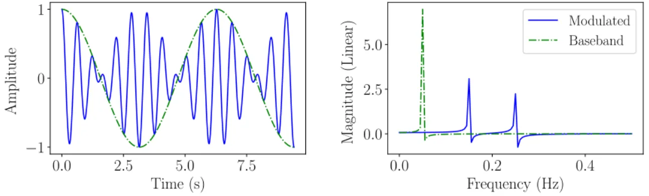
form of modulation is amplitude modulation, where the data signal is multiplied by a higher frequency sine wave, also known as a carrier. The resulting time and frequency domain signals are show in Figure 2.1, when the data signal is also a sine wave. A

sampling rate of 1 Hz is assumed to simply the scale and draw a stronger connection

to the Nyquist bandwidth. While simple, amplitude modulation is inefficient. It uses twice the spectrum required by the original signal, also known as the baseband signal,

0.0 2.5 5.0 7.5 Time (s) −1 0 1 A m p lit u d e 0.0 0.2 0.4 Frequency (Hz) 0.0 2.5 5.0 M ag n it u d e (L in ea r) Modulated Baseband

CHAPTER 2. BACKGROUND 0.0 2.5 5.0 7.5 Time (s) −1 0 1 A m p lit u d e 0.0 0.2 0.4 Frequency (Hz) 0 5 M ag n it u d e (L in ea r) Modulated Baseband

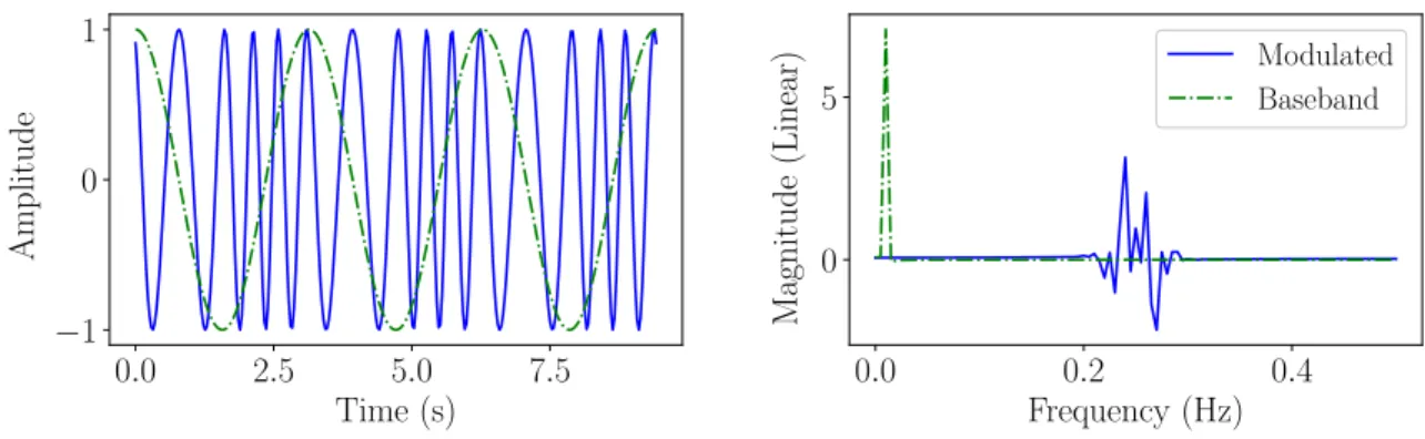
Figure 2.2: Frequency Modulation

and is not easy to demodulate. Improvements have been made, but it no longer sees widespread use for analog signals.

Frequency modulation, whose time and frequency domain outputs can be seen in Figure 2.2, is a more popular choice for analog signals. Instead of changing the amplitude of the carrier wave, frequency modulation varies the frequency. This results in increased spectrum use, but is more power efficient and is more noise resilient than amplitude modulation [20]. It continues to enjoy widespread use in FM radio broadcasts, as well as voice communication via two-way radio.

In order to modulate digital signals, bits must first be converted to symbols. The symbols are vectors in the complex plane, having both an in-phase part and a quadrature part. To reduce the bandwidth, a pulse shaping function is used. Finally, the shaped symbols are shifted up to the carrier frequency using a mixer, much like amplitude modulation, expressed as

s(t) = sI(t)cos(2πfct)₋sQ(t)sin(2πfct). (2.1)

s(t) is the transmitted signal, sI(t) and sQ(t) are the real and imaginary parts of the

symbol vector respectively, and fc is the carrier frequency.

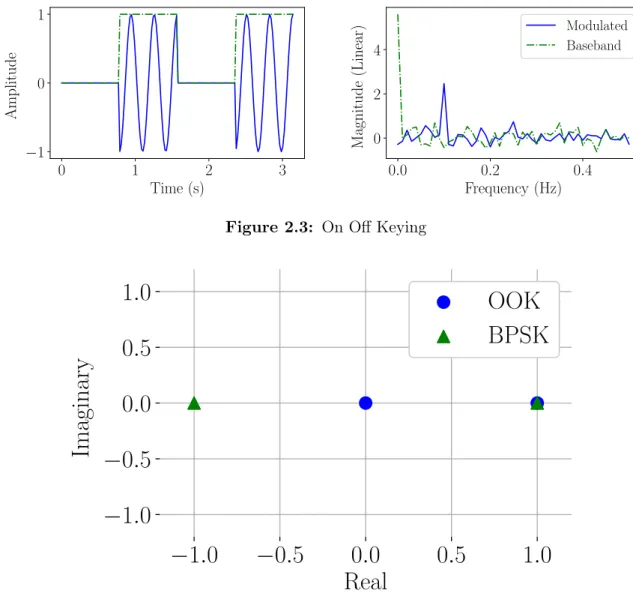
Generally, a modulation scheme will be referenced based on how it converts the bits to symbols. Perhaps the simplest example of this is On Off Keying (OOK). The

CHAPTER 2. BACKGROUND 0 1 2 3 Time (s) −1 0 1 A m p lit u d e 0.0 0.2 0.4 Frequency (Hz) 0 2 4 M ag n it u d e (L in ea r) Modulated Baseband

Figure 2.3: On Off Keying

−

1

.

0

−

0

.

5

0

.

0

0

.

5

1

.

0

Real

−

1

.

0

−

0

.

5

0

.

0

0

.

5

1

.

0

Im

ag

in

ar

y

OOK

BPSK

Figure 2.4: Symbol constellations

symbols are the same as the bits, meaning that ifb[k]is the bit at samplek,sI[k] =b[k]

and sQ[k] = 0. A time and frequency domain example is show in Figure 2.3. While easy, it requires infinite bandwidth in the theoretical case, and cannot encode more than one bit. Additionally, it has a DC offset before it is mixed with the carrier signal.

A better version of OOK is Binary Phase-Shift Keying (BPSK). To better un-derstand the improvement that BPSK offers over OOK, it is useful to look at the locations of the symbols on the complex plane. Figure 2.4 shows this type of plot, known as a symbol constellation.

CHAPTER 2. BACKGROUND

−

1

.

0

−

0

.

5

0

.

0

0

.

5

1

.

0

Real

−

1

.

0

−

0

.

5

0

.

0

0

.

5

1

.

0

Im

ag

in

ar

y

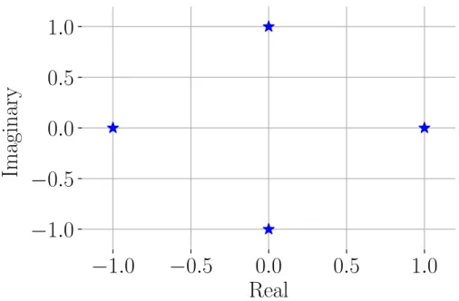
Figure 2.5: QPSK symbol constellation

Because the symbols will be affected by additive noise during transmission, they are unlikely to remain in the same position in the constellation plot after reception, but instead shift around randomly. The magnitude of the shift is related to the noise power, so the further distance between the symbols in BPSK means that it is more resilient.

Naturally, these are not the only two possibilities. Another option is Quadrature Phase-Shift Keying (QPSK), whose symbol constellation is given in Figure 2.5. Since there are four possible symbols, two bits can be encoded together, resulting in a doubling of the bit rate, assuming that everything else remains equal. However, this comes at a cost, since the symbols are closer together. This leads to an increased Bit Error Rate (BER) for the same SINR, where the BER is defined to be the number of bits per unit time that are incorrect [20]. Naturally, incorrect bits do not provide useful information, and thus do not increase the throughput. Ignoring any error correction, the system cannot be sure of which bit, or bits, was transmitted, so a retransmission is required, which further reduces the throughput. For this reason, QPSK is best used in systems with a somewhat high SINR.

CHAPTER 2. BACKGROUND −1.0 −0.5 0.0 0.5 1.0 Real −1.0 −0.5 0.0 0.5 1.0 Im ag in ar y (a) 16-QAM −1.0 −0.5 0.0 0.5 1.0 Real −1.0 −0.5 0.0 0.5 1.0 Im ag in ar y (b) 64-QAM

Figure 2.6: QAM symbol constellations

Both BPSK and QPSK use phase shifts to separate the symbols. This produces constellations with good separation up through four symbols, but beyond that, better schemes are possible. The most popular of these other schemes is Quadrature Amplitute Modulation (QAM), where the symbols are placed on a grid, which is centered around the origin. Constellations for 16-QAM and 64-QAM are shown in Figure 2.6.

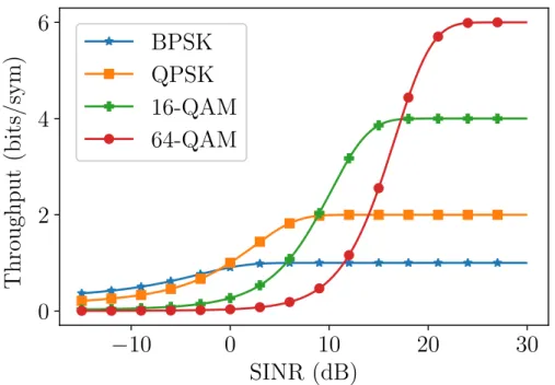
Since their separation is less than that of QPSK, they require even better SINR to achieve a low BER. For this reason, many systems, including WiFi, use adaptive modulation to send data quickly when possible, but still maintain communication when the noise power increases [21]. The modulation scheme chosen directly correlates with the SINR of the system, providing a method to gather information about the PU’s SINR without any interaction or possibility of interference, which is critical for underlay DSA.

2.4

Adaptive Modulation

Since different modulation schemes have higher throughputs at different SINRs, systems change, or adaptive their modulation scheme to fit the current SINR. The differing throughput values can be attributed to a combination of the maximum possible throughput and the BER at a specific SINR. At low SINRs, they use BPSK, as it is the most noise resilient, followed by QPSK, then 16-QAM, and finally 64-QAM.

CHAPTER 2. BACKGROUND

−

10

0

10

20

30

SINR (dB)

0

2

4

6

T

h

ro

u

gh

p

u

t

(b

it

s/

sy

m

)

BPSK

QPSK

16-QAM

64-QAM

Figure 2.7: Throughput as a function of SINR for WiFi modulation schemes

A possible throughput curve for WiFi is given in Figure 2.7. Notice that the maximum throughput levels off for brief periods. During this time, the current modulation scheme is able to be decoded with a very small error rate, but switching to a higher modulation would result in an increased number of errors, so the change is not done. It is clear that knowing the modulation scheme provides a rough estimate of the PU’s SINR. If the SU is allowed to send tones with a specific power, it can observe how the modulation scheme changes to get a finer resolution SINR estimate.

2.5

Cyclostationarity

Signals in communications are often said to be wide sense stationary, meaning that some of their statistical properties do not vary with time, meaning that

E[x] =E[x(t)], Rx(τ) =Rx(t, τ).

CHAPTER 2. BACKGROUND

The mean does not rely on the time, and the autocorrelation only changes when

the time shift, τ, is varied [20]. Perhaps the most popular signal with this model is

Additive White Gaussian Noise, whose mean is zero, and whose variance is related to the power of the noise, which is assumed to remain constant. However, not all signals fall so nicely into this category. Consider, for example, the moving average of a sine wave, where the averaging window is less than a period. The average will change over time, but will still be periodic, and thus can be modeled using a cyclostationary process. More formally, a process whose properties, such as mean and autocorrelation, vary periodically with time is known as a cyclostationary process [22]. Mathematically, this is expressed as

E[x(t)] =E[x(t+T0)], Rx(t, τ) = Rx(t+T0, τ).

While similar to the stationary definitions, these still rely on t, since periodicity

Chapter 3

Techniques for Modulation Classification

3.1

Fraction-of-Time Probability

Traditional probability theory is based on stochastic processes and in order to model data, samples of these processes must be taken from a population. This is reasonable, if the data in question are dice rolls, and the population is simply the six faces of a die. However, when no such population exists, as is the case in many of the real world signals that communications employ, this model does not work as well. Nevertheless, because of the prevalence of the stochastic model, engineers often choose to represent the data as a sample path of a stochastic process.

An alternative to this approach is to consider the Fraction-of-Time (FOT) proba-bility model. This model is based on the idea that the data to be modeled are derived from some process whose statistical parameters remain the same over a very long time period. By working with the infinite time series of the data, similar statistics, such as mean and variance can be calculated. These calculations are analogous to those in the stochastic framework, where an infinite amount of samples are instead required [23].

The expectation operator of the FOT framework is

Etβ{z(t)}, lim T→∞ 1 T Z T /2 −T /2 z(t₋u)ei2πβu_{du. (3.1)}

CHAPTER 3. TECHNIQUES FOR MODULATION CLASSIFICATION

center frequency isβ [24]. In other words, it extracts a single sine wave from the input

signal, z(t), much like the expectation operator can be used to find a single value in

an ensemble. Whenβ is set to zero, the sine wave extraction operator instead extracts

the average value from the data set, which is equivalent to finding the expected value. Because of this duality, the calculation of traditional statistics such as mean, variance, and other moments using FOT is mathematically valid [25].

3.2

Second-Order Cyclostationarity

Given the signal, x(t), the mathematical definition of autocorrelation is

Rxx(τ) =

Z ∞

−∞

x(t)x(t₋τ)dt (3.2)

assuming that the signal is stationary [20]. This can also be viewed as an expected value,

Rxx(t1, t2) = E[x(t1)x∗(t2)], (3.3)

which is more helpful for statistical signal processing. Here, no such assumption about stationarity is made, as time continues to be present in the arguments to the

autocorrelation function. After defining t= (t1+t2)/2 and τ =t1−t2,

Rxx(t, τ) =E[x(t+τ /2)x∗(t₋τ /2)]. (3.4)

This form is particularly useful because its Fourier coefficients make up the Cyclic Autocorrelation Function (CAF) [22], given by

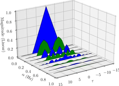
Rα x(τ) = lim T→∞ 1 T Z T /2 −T /2 x(t+τ /2)x∗(t−τ /2)e−i2παt_{dt. (3.5)}

CHAPTER 3. TECHNIQUES FOR MODULATION CLASSIFICATION τ −15 −10 −5 0 5 10 15 α (Hz) 0.0 0.2 0.4 0.6 0.8 1.0 M ag_n it u_d e (L in ea r) 0.0 0.2 0.4 0.6 0.8 1.0

Figure 3.1: Cyclic Autocorrelation Function for BPSK without pulse shaping

This form once again shows the connection between the two statistical frameworks, as

this could also be viewed as the sine wave extraction operator for x(t)x(t₋τ). In fact,

this view is quite reasonable, as the goal of the CAF is to find the cycle frequencies,

or α values which are non-zero. Each α value corresponds to a particular Fourier

coefficient, which means that α gives the frequency at which the autocorrelation

function contains some power. These values will arise from sine waves which are the naturally occurring product of two first order cyclostationary functions [25].

The CAF for a BPSK wave with no pulse shaping is shown in Figure 3.1. Note

that when α= 0 this is the traditional autocorrelation function, scaled by a factor.

This scaling factor results from the fact that the waveform contains power in other

cycle frequencies besidesα = 0.

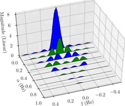
CHAPTER 3. TECHNIQUES FOR MODULATION CLASSIFICATION f (Hz) −0.4 −0.2 0.0 0.2 0.4 α (H z) 0.0 0.2 0.4 0.6 0.8 1.0 M ag_n it u_d e (L in ea r) 0 2 4 6 8

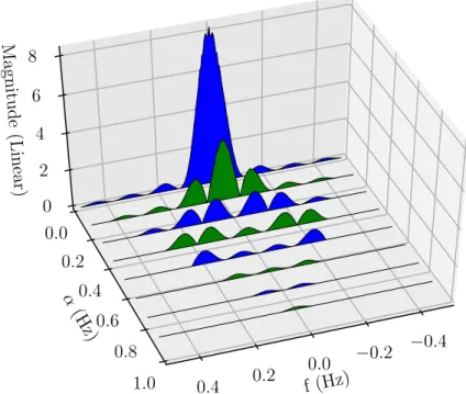
Figure 3.2: Spectral Correlation Function for BPSK without pulse shaping

Function (SCF), where Sα x(f) = Z ∞ −∞ Rα x(τ)e −i2πf τ_{dτ. (3.6)}

When the value of α is set to be zero, this gives the Wiener-Khinchin Theorem for

stationary processes [20]. The theorem states that the Power Spectral Density (PSD) for a stationary signal is equal to the Fourier Transform of the autocorrelation function. The same BPSK wave as in Figure 3.1 was used to create the SCF shown in

Figure 3.2. α = 0 is the PSD of the signal. Other non-zero values are present at

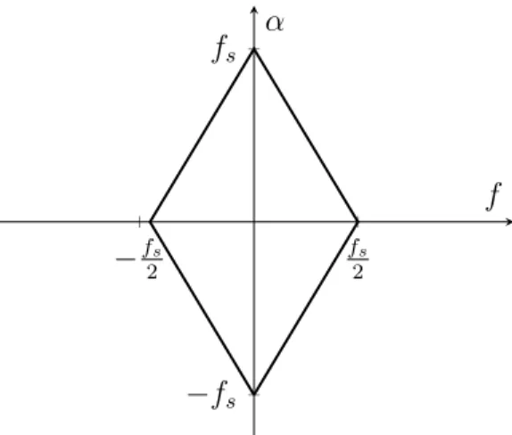
various cycle frequencies. Note that the region of support for the SCF is limited to

the region shown in Figure 3.3 [26]. fs represents the sampling frequency. This region

follows from the Nyquist bandwidth, since it limits the bandwidth of the signal to be

±fs/2 along the f-axis. By rewriting (3.6) as

Sα x(f) = lim T→∞Zlim→∞ 1 T Z Z Z/2 −Z/2 XT(t, f +α/2)XT∗(t, f −α/2)dt, (3.7)

CHAPTER 3. TECHNIQUES FOR MODULATION CLASSIFICATION −fs 2 fs 2 −fs fs f α

Figure 3.3: Region of support for the Spectral Correlation Function

the limits of theα-axis are made clear [13]. XT is the Fourier transform of x(t)and is

given by

XT(t, f) =

Z t+T /2

t−T /2

x(u)e−i2πf u_{du. (3.8)}

Since α is the frequency shift, and is divided by two, shifting more than α is not

possible, as that would exceed the bandwidth of the sampled signal. It is also worth

noting that the SCF is symmetric about thef axis, meaning that it contains the same

values forα and ₋α. This was exploited in [15] to reduce the number of calculations

required.

3.3

Higher-Order Cyclostationarity

Not all modulation schemes are distinguishable using the CAF, or the SCF. For example, compare Figure 3.2, showing the SCF of BPSK, with Figure 3.4, showing the SCF of QPSK. Despite using two different modulation schemes, they are not easily distinguishable. Thus, higher-order statistics, such as moments and cumulants, are required to determine the type of modulation in use. The lag product, defined as

Lx(t,τ)n= n

Y

j=1

CHAPTER 3. TECHNIQUES FOR MODULATION CLASSIFICATION f (Hz) −0.4 −0.2 0.0 0.2 0.4 α (H z) 0.0 0.2 0.4 0.6 0.8 1.0 M ag_n it u_d e (L in ea r) 0 2 4 6 8

Figure 3.4: Spectral Correlation Function for QPSK

is simply the time delayed product of x(t). The notation (_∗) indicates that the

conjugation is optional. An nth-order statistic may have up to n/2 conjugations,

where different conjugations will produce different values, leading to multiple outcomes for the same order. Taking the expected value of the lag product yields the Temporal Moment Function, given by

Rx(t,τ)n=E[Lx(t,τ)n]. (3.10)

This corresponds to the nth-order autocorrelation function, which when evaluated

with n = 2, is equal to (3.3). Similarly, the Cyclic Temporal Moment Function is

Rα x(t,τ)n = lim T→∞ 1 T Z T /2 −T /2 Rx(t,τ)ne−i2παt_{dt, (3.11)}

and generalizes the CAF given in (3.5). Since the integration limits approach infinity,

CHAPTER 3. TECHNIQUES FOR MODULATION CLASSIFICATION

While moments could be used for classification, better alternatives exist, especially when the radio scene has multiple signals [27]. This led to the use of cumulants, which are robust to noise and have the superposition property, like voltage sources in a circuit. The moments do not have this useful property [25]. The Temporal Cumulant Function is Cx(t,τ)n = X P " (−1)p−1_(p−1)! p Y j=1 Rx(t,τvj)|vj| # , (3.12)

and is calculated using lower-order moments. Alternatively, it can be written as

Cx(t,τ)n =Rx(t,τ)n− X P,p6=1 " _p Y j=1 Cx(t,τvj)|vj| # , (3.13)

which instead uses lower-order cumulants [28]. The summation is performed over P,

which is the set of all possible partitions of the set _{1,2, ..., n}, the counting numbers

up to n. For n = 3, the set to be partitioned is _{1,2,3}, and P is

P =_{{1,2,3_},

{{1},{2,3}},

{{1,3_},_{2_}},

{{1,2_},_{3_}}}

{{1},{2},{3}}}.

Each row is a different partition, meaning that it contains each element of the original

set in one and only one of the subsets. For example, the second partition,_{{1_},_{2,3_}},

has two subsets containing either 1, or 2 and 3. Compare this to the first partition,

{1,2,3}, where all three values are in the same subset. These variations are important

because they affect p, the number of subsets in each partition. For the prior P,

p={1,2,2,2,3}. Note that multiple partitions may have the same value of p, such

CHAPTER 3. TECHNIQUES FOR MODULATION CLASSIFICATION

summation. In (3.13), p= 1 is skipped because it is equal to the first term on the

right hand side. Finally, j indexes each partition, iterating through all of its subsets.

When the current partition is _{{1_},_{2,3_}}, j = 1 indicates the set _{1_}, and j = 2

references _{2,3_}. _|vj_| simply means the number of elements in the subset indexed by

j, being 1 and 2 for the previous example, representatively.

A 4th-order example is given next to clarify. For simplicity, the number of

conjugations is set to zero. Since it has been shown that odd order moments for most communication signals are zero [25], they will be ignored for the analysis, meaning that partitions containing sets with one or three elements are not included. One

such partition like this is _{{1_},_{2,3,4_}}. The first subset, where j = 1, has only one

element, so _|vj_| is also one. This results in the inclusion of Rx(t, τ1)1 in the product,

but this is no different than the mean of the signal, shifted by τ. The mean of the

possible symbol values, when all symbols are considered, for the modulation schemes discussed in Section 2.3, excluding OOK, is zero. If the symbol constellations are viewed as probability distributions, and each symbol is equiprobable, the mean for each can be calculated. For example, in QPSK, the possible symbol values, or probabilistic

outcomes, are _±i and _±1, so the mean is 1₄((1) + (₋1) + (i) + (₋i)) = 0. Because

the mean is zero, the product containing this moment will also be zero, and is thus ignored. Similar logic can be applied for the third-order moments, leaving only the

second and fourth-order moments. P is then:

P =_{{1,2,3,4_},

{{1,2},{3,4}},

{{1,3_},_{2,4_}},

{{1,4_},_{2,3_}}}.

CHAPTER 3. TECHNIQUES FOR MODULATION CLASSIFICATION

has only one subset, so p will equal one for this iteration. The other three partitions

all have two subsets, sop will be two in those iterations. Additionally, sincepis either

one or two, (p₋1)! is always one, and can be ignored. For clarify, the contribution of

each partition will be analyzed separately, and i will be used to indexP, the partition

list. For the four possible values of i, the contributions are:

i= 1 : (₋1)1−1_Rx(t, {τ1, τ2, τ3, τ4})₄ i= 2 : (−1)2−1_Rx(t,{τ 1, τ2})2Rx(t,{τ3, τ4})2 i= 3 : (₋1)2−1_Rx(t, {τ1, τ3})₂Rx(t,{τ2, τ4})₂ i= 4 : (−1)2−1Rx(t,{τ1, τ4})₂Rx(t,{τ2, τ3})₂.

The values of τ in each of the moments of a contribution correspond to the values in

that partition ofP. The second partition consists of two subsets: _{1,2} and _{3,4},

and thus two second-order moments. For the first moment, the τ values are _{τ1, τ2}

and_{τ3, τ4}for the second. This ensures that all possible combinations of the τ vector

are considered. For simplicity,τ is set to zero. The fourth-order cumulant resolves to

Cx(t,0)4 =Rx(t,0)4−3 (Rx(t,0)2) 2

.

This form is not yet useful, as it changes with time. By using the FOT expectation operation, the Cyclic Temporal Cumulant Function or cyclic cumulant, given by

Cα x(τ)n= lim T→∞ 1 T Z T /2 −T /2 Cx(t,τ)ne−i2παt_{dt, (3.14)}

can be calculated [28], and is the form that is used for modulation classification. Here,

α serves the same function that it does in the CAF, and is zero unless otherwise noted

for this work. Since this notation does not convey the number of conjugations, the

CHAPTER 3. TECHNIQUES FOR MODULATION CLASSIFICATION

Table 3.1: Second-order cumulants of QPSK x x2 _xx∗ 1 1 1 -1 1 1 i -1 1 −i -1 1 Sum 0 4

the number of conjugations. Notation with a hat, shown as Cnqˆ , denotes when the

cumulant is an estimate, instead of an exact value.

The importance of q, the number of conjugations, can be seen by considering a toy

example involving C20 and C21 of QPSK. Table 3.1 shows the outcomes of calculating

the two cumulants in question with and without the optional conjugation. Dividing

the sum ofx2 _andxx∗ _{by four produces the theoretical value ofC}

20andC21 for QPSK,

respectively.

As an alternative to these representations of moments and cumulants, they can be calculated from their deriving functions, given as

ΦX(ω) = Z ∞ −∞ fX(u)eiωu_du, MX =E[Xn_{] =} ∂n ∂ωnΦX(ω) ω=0 , (3.15) CX = ∂ n ∂ωnln (ΦX(ω)) ω=0 . (3.16)

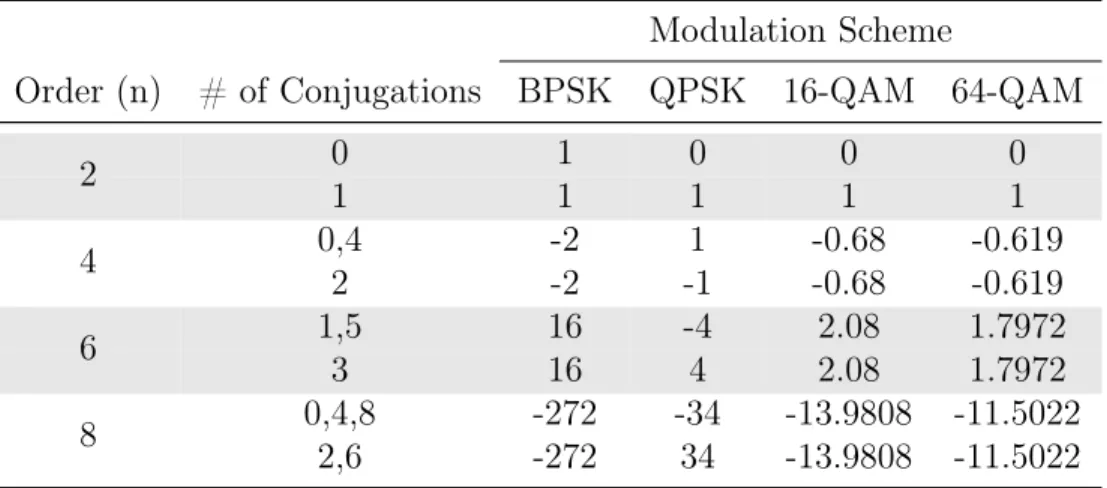
While not helpful for calculating the cumulant of a sample path, this form demonstrates why the value of a cumulant for a given probability distribution, or modulation scheme, is constant. The results of several such calculations are shown in Table 3.2 [29]. All calculations are done using a constellation of unit variance, which is reflected in the second row of the table. Since the symbols are normalized, the power of the signal is always one, which is equivalent to the second-order cumulant with one conjugation, as

CHAPTER 3. TECHNIQUES FOR MODULATION CLASSIFICATION

Table 3.2: Theoretical cumulant values for selected modulation schemes

Modulation Scheme

Order (n) # of Conjugations BPSK QPSK 16-QAM 64-QAM

0 1 0 0 0 2 1 1 1 1 1 0,4 -2 1 -0.68 -0.619 4 2 -2 -1 -0.68 -0.619 1,5 16 -4 2.08 1.7972 6 3 16 4 2.08 1.7972 0,4,8 -272 -34 -13.9808 -11.5022 8 2,6 -272 34 -13.9808 -11.5022

Chapter 4

Techniques for Undersampling

In order to undersample a signal, it must be sparse in some domain. This sparsity means that less samples are required to extract enough meaningful data from the signal in order to reconstruct it. An example of the compression process is given in

Figure 4.1. The x vector, or original signal, is sparse, as seen by the white squares.

At the output z, the signal is no longer sparse, having been compressed. The signal

is also in in the “dark” domain, having been both compressed and transformed by

Ψ

x

y

=

CHAPTER 4. TECHNIQUES FOR UNDERSAMPLING

the Φmatrix. For clarity, Φ is sometimes represented as AΨ, where Aperforms the

compression, and Ψ is the transformation matrix. Here, the compression matrix will

refer to the identity matrix with rows removed, but other options, such as Bernoulli or Gaussian matrices are possible [8]. Since the signal is no longer sparse, it can be efficiently sampled. The transformation performed is often the Fourier transform, but can also be a wavelet transform, or the DCT. Note that lowercase bold letter denote vectors, and upper case bold letters indicate matrices.

For the reconstruction to work, the sampling matrix, Φmust fulfill the Restricted

Isometry Property. This property is stated as

(1−δS)||c_||2_{2 ≤ ||}ΦSc||22 ≤(1 +δS)||c|| 2

2, (4.1)

and was first introduced in [30]. Here, ΦS is an S-large subset of the columns of Φ, c

is any real vector with length S, and _{|| · ||}2 takes the`2 vector norm of the argument.

As the constant δS approaches zero, the system begins to behave like an orthonormal

system, from which recovery is a straightforward task. In general, two forms are possible for the recovery equation. The traditional approach, in which sparsity is an afterthought, is given as,

arg min

x ||z−Φx||

2

2+λ||x||1. (4.2)

The sparsity constraint is enforced by the second term, and λ determines the level of

sparsity. The alternative method, known as basis pursuit, uses only the `1 norm, and

is shown as

arg min

x ||x||1 subject to Φx≈z. (4.3)

This method can be easily approximated using a greedy algorithm, as shown in Section 4.1, making it much faster to solve than (4.2).

CHAPTER 4. TECHNIQUES FOR UNDERSAMPLING

Algorithm 4.1 Orthogonal Matching Pursuit

Input: Dictionary D, signalz, target sparsity K or target error

1: I ← {}

2: r ←z

3: x_←0

4: while stopping criterion not met do 5: kˆ←arg maxˆ_khDˆ_k,ri

6: I ←(I,kˆ)

7: x_←D†_Iz

8: r _←z₋DIx

Output: x

4.1

Orthogonal Matching Pursuit

Orthogonal Matching Pursuit (OMP) is one such greedy algorithm. Originally derived in [31], OMP enforces sparsity by adding values one at a time until either a desired sparsity level is reached, or the residual falls below a specified threshold. Algorithm 4.1 details the implementation of OMP. In order to reduce the residual as fast as possible,

the inner product, denoted _h·,·i, is taken between the residual and the dictionary.

The maximum value of the inner product is produced by the basis vector that is most

in line with the current residual. The index of this basis vector is denoted ˆk, and

added to I. I is then used to index D, whose pseudoinverse is multiplied with the

input signal z, giving the current reconstruction. This reconstruction is then tested

against the signal to determine if the error stopping criteria has been met. While the pseudoinverse can be computationally difficult, here it is fairly efficient, due to the fact that each iteration only adds a column, so the previous pseudoinverse can be applied to speed up the computation [32].

In the specific case of cumulant reconstruction, the calculation of the pseudoinverse can be further optimized to increase the amount of possible preprocessing. The first, and most important, optimization is the removal of the loop. In order to justify this,

CHAPTER 4. TECHNIQUES FOR UNDERSAMPLING

z, occurs in the first column more than 98% of the time. To take advantage of this,kˆ

was set to 1. Additional iterations are not required, as only one cycle frequency is needed to perform the classification.

Without knowing the number of iterations, or which columns would be selected,

2n_{−1pseudoinverses would be required, where n is the number of columns in D. If}

the columns ofDare considered a set, there are 2n_{possible subsets, but a column will}

always be selected, so the empty set can be ignored. In the single iteration case, DI

will contain a single column, so n pseudoinverses have to be precomputed. However,

because ˆk = 1, only one pseudoinverse needs to be found. Thus, the optimization

removes almost all of the complexity associated with the precomputation of the pseudoinverse(s).

These pseudoinverses are fairly straightforward to calculate, but require a division operation, which can be quite expensive. However, this operation can be eliminated by considering the Moore-Penrose pseudoinverse, given by

D†_I = (D_I∗DI)−1D∗I, (4.4)

when DI is a single column. D∗ denotes the Hermitian, or conjugate, transpose of

the matrix. DI is only one column wide, so

D∗D=_||DI||22, (4.5)

whose inverse is simply the multiplicative inverse. The pseudoinverse then collapses to D_I†= D ∗ I ||DI||22 , (4.6)

which is simply a row vector. Reconstruction is performed by multiplying D_I† with z,

which is the same as the dot product between D†_I

T

Chapter 5

Using Cumulants to Classify Modulation Schemes

5.1

Methods of Estimation

Three primary methods were chosen for cumulant estimation: direct, Fourier Transform,

and CS. An estimator of the n-th order moment is given in Equation (5.1), which is

required for the direct method equations given as

ˆ Mn= 1 N N X i=1 zn_{[i], (5.1)} ˆ C40= ˆM4−3 ˆM22, (5.2) ˆ C80= ˆM8−28 ˆM6Mˆ2−35 ˆM42+ 420 ˆM4Mˆ22+ ˆM 4 2. (5.3)

In order to simplify the design of the CS estimator, only the cumulants without conjugations were calculated. This has been done in the past and shown to produce a successful classifier [33].

A visual representation of the Cˆ40 estimator is shown in Figure 5.1. Note that this

process is iterative and the estimate improves as more samples are obtained. Once the desired number of samples is obtained, the iteration stops, and the final estimate is calculated. The only computations that need to be performed after all of the samples are obtained are a squaring operation, multiplication by a constant, and one addition.

CHAPTER 5. USING CUMULANTS TO CLASSIFY MODULATION SCHEMES zi (·)2 _(·)2 _{+ N}−1 + N−1 (·)2 ₋₃ + ˆ C40 ˆ C20

Figure 5.1: Estimation of the 4th-order cumulant value

z (_·)2 _(·)2 FFT FFT (·)2 −3 + Cˆα 40 ˆ C20

Figure 5.2: Estimation of the 4th-order cumulant value using FFTs

(FFT) and is outlined in Figure 5.2 for Cˆα

40. Because an FFT is used, the entire

sample path must be obtained before calculations can start. Notice also, that all

Fourier coefficients, as indicated by the α, are calculated, instead of the singular

coefficient in the case of the direct method. These extra coefficients are seldom used for classification and are discarded in this method.

Although the Fourier Transform approach calculates extraneous information, it is a building block for the CS method. If the transform is performed using a matrix, the cumulant can be estimated by

ˆ

C40α =F[[z]] 4

−3[[F[[z]]2]]2. (5.4)

[[_·]]n _{indicates the element-wise power operation and F is the Fourier Transform}

matrix. Since the first row of this matrix has all elements equal to _N1, the first element

of Cˆα

CHAPTER 5. USING CUMULANTS TO CLASSIFY MODULATION SCHEMES

were some inconsistencies, so the full derivation of the CS method is shown. First, the incoming samples are compressed via

z=Ax, (5.5)

where A is an M_×N compression matrix discussed in Chapter 4.

DefiningR[[x]] to be the autocorrelation matrix, also given byE[xxH], even powers

of the samples can be found, such as:

[[x]]4 =diag R[[x]]2

=Pxvec R[[x]]2

. (5.6)

A row selection matrix, Px ∈ {0,1}N×N

2

, removes the unneeded autocorrelation

matrix entries, and the vec(_·)operation stacks the columns of the argument to form

an N2_{×1 vector. Other variants of P are also required, such as P}

z, which is an

M ×M2 _{matrix that performs the same function.}

The relationship between the compressed and non-compressed autocorrelation

matrices, which requires removing the rows and columns not present in z, is given as,

R[[z]]2 =AR_[[x]]2AT. (5.7)

Because theP matrix acts upon vectors, instead of matrices, the vectorizing operation

is performed, which when combined with the identity that states vec(ABC) =

(CT _{⊗A)vec(B), where⊗ denotes the Kronecker product, produces}

vec R[[z]]2

= (A_⊗A)vec R[[x]]2

CHAPTER 5. USING CUMULANTS TO CLASSIFY MODULATION SCHEMES

Combining Equations (5.4) through (5.8) leads to:

ˆ Cα 40 =F Pxvec R[[x]]2 −3PFxvec RF[[x]]2 , =F Pxvec R[[x]]2−3P_F xvec F R[[x]]2F T , = [F Px−3PFx(F ⊗F)]vec R[[x]]2 . (5.9)

Finally, the matrix inside the brackets is inverted, and (5.8) applied to produce

[[z]]4 _=P

z(A⊗A) [F Px−3PFx(F ⊗F)]

† _ˆ

Cα

40. (5.10)

This matches the traditional CS problem when only [[z]]4 _{is known and Φis equal to}

Pz(A⊗A) [F Px−3PFx(F ⊗F)]

† .

5.2

Method of Decision

A Bayesian hypothesis test was performed to determine which of the modulation schemes the unknown signal was using. To simplify the decision making process, only the two cumulants whose theoretical values were closest to the estimate were considered. This reduced the problem to a binary hypothesis test, and allowed the application of P(x|w1) P(x_|w2) w1 ≷ w2 P(w2) P(w1) . (5.11)

Finding P(x|w1) was done empirically by plotting the values of the cumulants to

determine which distribution was most appropriate. If the variance was required for the selected distribution, e.g. Gaussian, it was estimated using

σ2 z = 1 N −1 N X i=1 (zi₋µz)2_{. (5.12)}

CHAPTER 5. USING CUMULANTS TO CLASSIFY MODULATION SCHEMES z(t) ADC Cumulant Estimator Preliminary Modulation Selector Final Modulation Selector Prediction

Figure 5.3: Block diagram of the modulation classifier

The a priori probabilitiesP(w1)andP(w2)were both assumed to be 0.5, as no further

information was estimated to influence them. The output of this decision was then used as the prediction of the detector, which was compared against ground truth to determine if it had decided correctly. Figure 5.3 shows the complete system. The preliminary selector performs the conversion to a binary hypothesis test, while the final selector uses the Bayesian hypothesis test to determine the output.

5.3

Approach

In order to determine the most promising way to implement modulation classification using cumulants, each method was implemented and tested using simulations. First, comparisons between two different orders, 4 and 8, were performed. There has been an increasing amount of research in recent years regarding higher order cumulants [35] [36] [37]. This is because they have been shown to be more discriminating, especially with higher order modulation schemes such as 16-QAM and 64-QAM or even 256-QAM, as is made clear by Table 3.2.

Two cumulants, Cˆ40 and Cˆ80 were chosen for the initial investigation. Their

performance in different scenarios, such as number of samples, SINR, carrier offset,

and phase shift, were considered. In addition to the probability of deteection (PD) each

cumulant achieved, a metric was added for Cˆ80 to determine how often it successfully

classified a set of samples thatCˆ40 did not. This provided insight into the performance

gain that was achievable using 8th-order cumulants that could not be obtained with the 4th-order ones.

CHAPTER 5. USING CUMULANTS TO CLASSIFY MODULATION SCHEMES

Having selected Cˆ40, the analysis continued by comparing the direct and FFT

approaches. Finally, the CS approach was included. For the CS approach, two methods of reconstruction were considered, convex optimization and OMP. Initially, these two methods were pit against one another, and then the better algorithm was tested against the direct method of cumulant calculation.

Chapter 6

Results and Analysis

WiFi was chosen as the target networking standard for this research. It is very prolific, meaning that there are plenty of opportunities for spectrum reuse, as well as being well documented, for ease of development. However, it also presents a few challenges. Most notably is the use of Orthogonal Frequency Division Multiplexing (OFDM), which divides the channel bandwidth into many smaller bandwidth channels.

Individual channels then send low rate symbols independently and in parallel, and those symbols are then placed back into a serial stream by the receiver. This presents many advantages in terms of throughput and bit error rate, but makes AMC more difficult by masking which modulation scheme is in use. Fortunately, it is possible to extract a single channel from the OFDM signal [38] [39]. This step is not covered, however the effects of doing so, such as a phase shift or carrier frequency offset were investigated. The four modulation schemes considered were BPSK, QPSK, 16-QAM, and 64-QAM. A listing of their cumulants is given in Table 3.2.

6.1

Distributions and Variances

In order to determine the distribution of the cumulant estimates, 10000 estimates of random inputs were found and plotted after being scaled to be a Probability Density Function. One such plot can be seen using the direct method in Figure 6.1. The distributions appear to be normal, supporting the proof given in [40], so that was

CHAPTER 6. RESULTS AND ANALYSIS −4 −3 −2 −1 0 0.0 0.2 0.4 0.6 σ2_{= 0.35158} BPSK 0.8 0.9 1.0 1.1 0 5 10 15 20 σ2_{= 0.00080} QPSK −0.9 −0.8 −0.7 −0.6 −0.5 −0.4 0 2 4 6 σ2_{= 0.00377} 16-QAM −0.8 −0.6 −0.4 0 2 4 6 σ2_{= 0.00490} 64-QAM

Best fit Gaussian Estimates

Figure 6.1: Distribution of cumulant estimates using the direct method

chosen as the distribution to use in Equation (5.11).

While the variances are not equal, the 16-QAM variance is smaller. This means that using Equation (5.11) with the experimental variances would result in an increase in the number of errors associated with 16-QAM, and a decrease in the 64-QAM errors. This shift is undesirable in the application of underlay DSA as described in Chapter 2. A misclassification of 16-QAM as 64-QAM would inform the system that the PU is performing better than it really is, which may cause the SU to raise its transmit power above an acceptable level. More generally, the BER of a system remains approximately constant when using adaptive modulation, but the throughput varies with the SINR. Increasing the SINR of the channel forces the system to lower its throughput in order to maintain an acceptable BER without increasing transmit power. In the underlay DSA situation, this SINR increase comes from the SU’s transmissions. A smaller SINR increase, which would come from misclassifying 64-QAM as 16-QAM, would affect the BER less, and thus lead to a smaller, or nonexistent, drop in PU throughput.

CHAPTER 6. RESULTS AND ANALYSIS

Naturally, this is also not desirable, but it is a better outcome than the first case. For this reason, it was assumed that the variances were equal for all modulation schemes across all cases. The theoretical values of BPSK and QPSK are too far away to factor into this issue. As will be shown, they are rarely misclassified, even at low SINRs or sample sizes.

6.2

Classification without Signal Impairments

The performance of the estimators was first assessed when there was no phase shift, carrier frequency offset, or noise. Instead, the number of samples was varied to determine how well the estimators would work when they undersampled the signal.

Note that true compression, where N samples are gathered and only M are used

(N > M), was not performed. Because the estimators do not improve if multiple samples of the same symbol are provided, the number of symbols input to the estimator was simply decreased. Nevertheless, the standard compression ratios are still useful. This work uses 1000 samples as a compression ratio of 1.

The first comparison was between the direct methods for Cˆ40 andCˆ80, as shown in

Figure 6.2. The two lines near the top represent the estimators raw performance. On

the bottom is a line with starred markers that shows the cases where Cˆ80 successfully

classified the modulation scheme, but Cˆ40 did not. This indicates the improvement

ˆ

C80 offers above Cˆ40, which is quite minimal for this case. More precisely, Cˆ80 offers

no improvement over Cˆ40 in the case of 16-QAM, and only a 2% increase in accuracy

when classifying 64-QAM.

The FFT and direct method for Cˆ40 were then compared, and the plots shown in

Figure 6.3. As expected, there is no difference between the two methods, so the extra overhead of calculating the various frequencies is not required.

The effectiveness of the two methods of reconstruction, convex optimization and OMP is shown in Figure 6.4. Both methods fail to classify BPSK, as they are only

CHAPTER 6. RESULTS AND ANALYSIS 0 2500 5000 7500 10000 0.00 0.25 0.50 0.75 1.00 PD BPSK 0 2500 5000 7500 10000 0.00 0.25 0.50 0.75 1.00 QPSK 0 2500 5000 7500 10000 0.00 0.25 0.50 0.75 1.00 PD 16-QAM 0 2500 5000 7500 10000 0.00 0.25 0.50 0.75 1.00 64-QAM Sample Count Sample Count C40 C80 C80only

Figure 6.2: C40 versusC80 as a function of sample count

0 2500 5000 7500 10000 0.00 0.25 0.50 0.75 1.00 PD BPSK 0 2500 5000 7500 10000 0.00 0.25 0.50 0.75 1.00 QPSK 0 2500 5000 7500 10000 0.00 0.25 0.50 0.75 1.00 PD 16-QAM 0 2500 5000 7500 10000 0.00 0.25 0.50 0.75 1.00 64-QAM Sample Count Sample Count No FFT FFT FFT only

CHAPTER 6. RESULTS AND ANALYSIS 0 200 400 0.00 0.25 0.50 0.75 1.00 PD BPSK 0 200 400 0.00 0.25 0.50 0.75 1.00 QPSK 0 200 400 0.00 0.25 0.50 0.75 1.00 PD 16-QAM 0 200 400 0.00 0.25 0.50 0.75 1.00 64-QAM Sample Count Sample Count OMP Comp Comp only

Figure 6.4: C40 with ideal reconstruction versus greedy method

Table 6.1: Powers of BPSK and QPSK

Symbol x2 _x4

-1 1 1

1 1 1

-i -1 1

i -1 1

provided with x4_{, which is indistinguishable from QPSK, as shown in Table 6.1. There}

is no difference in BPSK and QPSK when they are raised to the fourth power. To

overcome this, Cˆ20 was used, and its output is shown in Figure 6.5. This is very

successful, even at lower sample counts, as was the OMP reconstruction method. The performance in the 64-QAM case for the OMP method is best explained with the confusion matrices shown in Table 6.2. Across the top of the table are the correct modulation schemes, and the side labels indicate which scheme was predicted. This means that in the 10 sample case, the classifier predicts 64-QAM for both 16-QAM and 64-QAM, with little regard for the true modulation scheme. Unfortunately, this is

CHAPTER 6. RESULTS AND ANALYSIS 20 40 60 80 100 0.00 0.25 0.50 0.75 1.00 PD BPSK 20 40 60 80 100 0.00 0.25 0.50 0.75 1.00 QPSK Sample Count C20

Figure 6.5: C20for BPSK versus QPSK classification

Table 6.2: Confusion matrices for OMP reconstructions

(a)10 samples BPSK QPSK 16-QAM 64-QAM BPSK 0.004 0 0.283 0.206 QPSK 0.996 1 0.015 0.004 16-QAM 0 0 0.015 0.024 64-QAM 0 0 0.687 0.766 (b) 512 samples BPSK QPSK 16-QAM 64-QAM BPSK 0 0 0 0 QPSK 1 1 0 0 16-QAM 0 0 0.819 0.337 64-QAM 0 0 0.181 0.663

not correctable by modifying the thresholds, as shown by Figure 6.6. Because 64-QAM is correct half of the time, this leads to better than expected performance. At 512 samples, this is not the case, and the classifier is behaving much more reasonably.

The single column optimization, described in Section 4.1, was then tested against the standard OMP method to ensure that the computational optimization did not reduce the accuracy. Figure 6.7 shows the difference. This change results in comparable performance for all cases except 64-QAM at extremely low sample counts, but those estimates were not reliable to start.

CHAPTER 6. RESULTS AND ANALYSIS 2.5 5.0 7.5 10.0 12.5 0.0 0.5 1.0 1.5 σ2_{= 3.41713} BPSK 2.5 5.0 7.5 10.0 12.5 0.00 0.25 0.50 0.75 1.00 1.25 σ2_{= 0.66641} QPSK −10.0 −7.5 −5.0 −2.5 0.0 0.0 0.5 1.0 1.5 _σ2_{= 1.22423} 16-QAM −10.0 −7.5 −5.0 −2.5 0.0 2.5 0.0 0.5 1.0 1.5 σ2_{= 1.14145} 64-QAM

Best fit Gaussian Estimates

Figure 6.6: Variances of 10 sample estimates

0 200 400 0.00 0.25 0.50 0.75 1.00 PD BPSK 0 200 400 0.00 0.25 0.50 0.75 1.00 QPSK 0 200 400 0.00 0.25 0.50 0.75 1.00 PD 16-QAM 0 200 400 0.00 0.25 0.50 0.75 1.00 64-QAM Sample Count Sample Count Zero Freq. Largest Corr. Largest Corr. only

CHAPTER 6. RESULTS AND ANALYSIS 0 200 400 0.00 0.25 0.50 0.75 1.00 PD BPSK 0 200 400 0.00 0.25 0.50 0.75 1.00 QPSK 0 200 400 0.00 0.25 0.50 0.75 1.00 PD 16-QAM 0 200 400 0.00 0.25 0.50 0.75 1.00 64-QAM Sample Count Sample Count Direct OMP OMP only

Figure 6.8: C40 with direct versus greedy method

Figure 6.8. As expected, the OMP method fails to classify the BPSK. However, it performs the same in QPSK, and offers a significant improvement in the 16-QAM case.

6.3

Classification with Noise

Using 500 samples, which corresponds to approximately 75% accuracy in the noiseless case, the performance of the two methods was compared across a range of SINR values

from 0 dB to 30 dB. This range was chosen to match the SINR range over which

WiFi is specified to operate [21]. Figure 6.9 compares the performance of Cˆ40 against

ˆ

C80. Similar to the noiseless case, Cˆ80 offers little improvement over Cˆ40. This was

expected, since cumulants are generally considered to be resilient to noise.

Having shown that the FFT method and the convex optimization reconstruction are not useful using the samples test, they were not evaluated further. OMP was then tested against the direct method, once again using 500 samples, and the results are

CHAPTER 6. RESULTS AND ANALYSIS 0 10 20 30 0.00 0.25 0.50 0.75 1.00 PD BPSK 0 10 20 30 0.00 0.25 0.50 0.75 1.00 QPSK 0 10 20 30 0.00 0.25 0.50 0.75 1.00 PD 16-QAM 0 10 20 30 0.00 0.25 0.50 0.75 1.00 64-QAM SINR (dB) SINR (dB) C40 C80 C80only

Figure 6.9: C40 versusC80 as a function of SINR

given in Figure 6.10. As was the case with Cˆ80, no change in performance was noted

CHAPTER 6. RESULTS AND ANALYSIS 0 10 20 30 0.00 0.25 0.50 0.75 1.00 PD BPSK 0 10 20 30 0.00 0.25 0.50 0.75 1.00 QPSK 0 10 20 30 0.00 0.25 0.50 0.75 1.00 PD 16-QAM 0 10 20 30 0.00 0.25 0.50 0.75 1.00 64-QAM SINR (dB) SINR (dB) Direct OMP OMP only

Figure 6.10: Direct versus OMP as a function of SINR

6.4

Frequency and Phase Shifts

Traditional modulation estimation schemes rely on preprocessing steps to remove Carrier Frequency Offset (CFO) and phase shifts [41]. Since the estimators considered do not have any preprocessing, the predictions are poor, as seen by the results in Figure 6.11 and Figure 6.13. The excellent classification of 64-QAM is only because the system guesses 64-QAM nearly every time, as seen by Table 6.3. To understand why this occurs, it is helpful to see the distribution of the cumulant estimates, as shown in Figure 6.12. This behavior stems from the fact that a frequency shift is also

Table 6.3: Confusion matrix for a -0.0005 HzCFO

BPSK QPSK 16-QAM 64-QAM

BPSK 0 0 0 0

QPSK 0 0 0 0

16-QAM 0 0 0 0

CHAPTER 6. RESULTS AND ANALYSIS −0.0010−0.0005 0.0000 0.0005 0.0010 0.00 0.25 0.50 0.75 1.00 PD BPSK −0.0010−0.0005 0.0000 0.0005 0.0010 0.00 0.25 0.50 0.75 1.00 QPSK −0.0010−0.0005 0.0000 0.0005 0.0010 0.00 0.25 0.50 0.75 1.00 PD 16-QAM −0.0010−0.0005 0.0000 0.0005 0.0010 0.00 0.25 0.50 0.75 1.00 64-QAM Frequency (Hz) Frequency (Hz) C40 C80 C80only

Figure 6.11: C40ˆ versusC80ˆ as a function of CFO

−4 −2 0 2 4 ×10−6 0 100000 200000 300000 σ2_{= 0.00000} BPSK −1.0 −0.5 0.0 0.5 1.0 ×10−6 0 1000000 2000000 σ 2_{= 0.00000} QPSK −0.1 0.0 0.1 0 2 4 6 8 _σ2_{= 0.00255} 16-QAM −0.1 0.0 0.1 0.2 0 2 4 6 σ2= 0.00369 64-QAM

Best fit Gaussian Estimates

CHAPTER 6. RESULTS AND ANALYSIS 0 π/4 π/2 0.00 0.25 0.50 0.75 1.00 PD BPSK 0 π/4 π/2 0.00 0.25 0.50 0.75 1.00 QPSK 0 π/4 π/2 0.00 0.25 0.50 0.75 1.00 PD 16-QAM 0 π/4 π/2 0.00 0.25 0.50 0.75 1.00 64-QAM Phase Phase C40 C80 C80only

Figure 6.13: Cˆ40 versusCˆ80 as a function of phase shifts

a phase shift by a continuously varying amount. Each symbol in BPSK is rotated a little further than the previous, leading to a constellation that does not have any repeated symbols, which means that it is uniform. Furthermore, this distribution is approximately circular, so the zero-valued cumulants are expected [42]. Of the four cumulant values listed in Table 3.2, 64-QAM at -0.619 is closest to zero, so it is selected.

A simple phase rotation is also considered, and the results are shown in Figure 6.13.

Once again, the results are not good. Although the Cˆ80 produces better results, it

is in no way a reliable classifier, and it would be better to simply perform the phase correction before attempting to determine the modulation scheme.

6.5

Computational Efficiency

The accuracy of the different methods is naturally important, but the computing cost to execute the different algorithms should also be considered when selecting one for

CHAPTER 6. RESULTS AND ANALYSIS

use. When such algorithms are implemented in hardware, e.g. an FPGA or an ASIC, the more complex ones will take more area, driving up cost and energy consumption. Additionally, a complex algorithm takes more time to run, so results are delayed, which means that the cognitive radio cannot make decisions as quickly.

In order to help inform a decision about which algorithm to choose, the Cˆ40

direct,Cˆ80 direct, and OMP methods were analyzed to determine their computational

efficiency. The metrics considered were required number of resources, such as adders and multipliers, memory, and latency after receiving the last sample. Additionally, possible parallel operations are noted, and the reduction in latency foun