Robustness,
Information-Processing Constraints, and the
Current Account in Small Open
Economies
Yulei Luo, Jun Nie, and Eric R. Young
December 2010
Robustness, Information-Processing Constraints, and the Current
Account in Small Open Economies
Yulei Luo† University of Hong Kong
Jun Nie‡
Federal Reserve Bank of Kansas City Eric R. Young§
University of Virginia December 2010
RWP 10-17
Abstract
We examine the effects of two types of informational frictions, robustness (RB) and finite information-processing capacity (called rational inattention or RI) on the current account, in an otherwise standard intertemporal current account (ICA) model. We show that the interaction of RB and RI has the potential to improve the model’s predictions on the joint dynamics of the current account and income: (i) the contemporaneous correlation between the current account and income, (ii) the volatility and persistence of the current account in small open emerging and developed economies. In addition, we show that the two informational frictions could also better explain consumption dynamics in small open economies: the impulse responses of consumption to income shocks and the relative volatility of consumption growth to income growth. Calibrated versions using detection probabilities fit the data better along these dimensions than the standard model does.
Keywords: Robustness, Rational Inattention, Consumption Smoothing, Current Account, Detection Error Probabilities
JEL Classification: C61, D81, E21.
∗ We would like to thank Paul Bergin, Larry Qiu, Kevin Salyer, Tom Sargent, Ulf S¨oderstr¨om, Lars Svensson, and seminar participants at UC Davis, Iowa, the European Central Bank, the Sveriges Riksbank, University of South Carolina at Columbia, 2010 Federal Reserve System Macro Meeting, and Federal Reserve Bank of Kansas City for helpful comments and suggestions. Luo thanks the HKU seed funding program for basic research for financial support. Nie thanks Li Yi for the research assistance. Young thanks the University of Virginia Faculty Summer Grant Program for financial support. All errors are the responsibility of the authors. The views expressed here are the opinions of the authors only and do not necessarily represent those of the Federal Reserve Bank of Kansas City or the Federal Reserve System.
†School of Economics and Finance, University of Hong Kong, Hong Kong. Email address: [email protected]. ‡Economic Research Department, Federal Reserve Bank of Kansas City. E-mail: [email protected].
1
Introduction
Current account models following the intertemporal approach feature a prominent role for the behavior of aggregate consumption. For given total income, consumption is the main deter-minant of national saving, and the balance of national saving in excess of investment is the major component of current account. This important role for consumption has naturally led researchers to study current account dynamics using consumption models.1 For instance, the standard intertemporal current account (ICA) model is based on the standard linear-quadratic permanent income hypothesis (LQ-PIH) model proposed by Hall (1978) under the assumption of rational expectations (RE). Within the PIH framework, agents can borrow in the interna-tional capital market and optimal consumption is determined by permanent income rather than current income; consequently, permanent income also matters for the current account. For ex-ample, consumption only partly adjusts to temporary adverse income shocks, which makes the current account tend to be in deficit. In contrast, consumption fully adjusts to permanent in-come shocks, with little impact on the current account. We adopt Hall’s LQ-PIH setting in this paper because the main purpose of this paper is to examine the implications of two types of in-formation frictions, robustness and rational inattention, for the dynamics of the current account, and it is much more difficult to study these information frictions in non-LQ frameworks.2
However, many empirical studies show that the RE-ICA models are often rejected in the post-war data.3 It is not surprising that the standard RE-ICA models are rejected because the underlying standard permanent income models have encountered their own well-known empiri-cal difficulties, particularly the well-known ‘excess sensitivity’ and ‘excess smoothness’ puzzles. Specifically, the main problems with the standard RE-ICA models are as follows. First, the models cannot generate low contemporaneous correlations between the current account and net income. (Net income is defined as output less than investment and government spending.) If net income is a unit root or a persistent AR(1) process, the current account is perfectly correlated with net income, whereas in the data they are only weakly correlated (Aguiar and Gopinath 2007, Uribe 2009).4 Second, they cannot generate low persistence of the current account. The standard RE models predict that the current account and net income have the same degree
1
See Obstfeld and Rogoff (1995) for a survey.
2See Hansen and Sargent (2007a) and Sims (2003, 2006) for detailed discussions on the difficulties in solving
the non-LQ models with these information imperfections. The primary alternative model is based on Mendoza (1991), a small open economy version of a real business cycle model. That model would be significantly less tractable than the one we use, because it involves multiple state variables.
3
See Sheffrin and Woo (1990), Ghosh (1995), Glick and Rogoff (1995), Obstfeld and Rogoff (1996), Bergin and Sheffrin (2000), Nason and Rogers (2003), and Gruber (2004).
4
It is well known that given the length and structure of the data on real GDP, it is difficult to distinguish persistent trend-stationary AR(1) and difference-stationary (DS) processes for real GDP. We focus on the AR(1) case in this paper; the results for the DS case are available from the authors upon request.
of persistence, whereas in the data the persistence of the current account is much lower than that of net income. Third, the models cannot generate observed excess volatility of the current account (Bergin and Sheffrin 2000; Gruber 2004). Fourth, they cannot generate volatile con-sumption growth and the observed hump-shaped impulse responses of concon-sumption to income (Aguiar and Gopinath 2007). Finally, the assumption of certainty equivalence in these models ignore some important channels through which income shocks affect the current account. As shown in Ghosh and Ostry (1997) in post-war quarterly data for the US, Japan, and the UK, the current account is positively correlated with the amount of precautionary savings generated by uncertainty of future net income.
It is, therefore, natural to turn to new alternatives to the standard RE-ICA model and ask what implications they have for the joint dynamics of consumption, the current account, and income. In this paper, we examine how the two types of information imperfections, a preference for robustness and information-processing constraints (rational inattention, RI), can improve the model’s predictions on these important dimensions we discussed above. Hansen and Sargent (1995, 2007a) first introduce robustness (a concern for model misspecification) into economic models. In robust control problems, agents are concerned about the possibility that their model is misspecified in a manner that is difficult to detect statistically; consequently, they choose their decisions as if the subjective distribution over shocks was chosen by a malevolent nature in order to minimize their expected utility (that is, the solution to a robust decision-maker’s problem is the equilibrium of a max-min game between the decision-maker and nature). Robustness models produce precautionary savings but remain within the class of LQ-Gaussian models, which leads to analytical simplicity.5 We show that incorporating robustness can improve the model by along the following three dimensions in all small open countries: generating lower contemporaneous correlation between the current account and net income, lower persistence of the current account, and higher relative volatility of consumption growth to income growth. However, RB by itself fails to generate volatile current accounts and the hump-shaped impulse responses of consumption to income shocks.
Sims (2003) first introduced rational inattention (RI) into economics and argued that it is a plausible method for introducing sluggishness, randomness, and delay into economic models. In his formulation agents have finite Shannon channel capacity, limiting their ability to process signals about the true state of the world. As a result, an impulse to the economy induces only gradual responses by individuals, as their limited capacity requires many periods to discover just how much the state has moved; one key change relative to the RE case is that consumption
5A second class of models that produces precautionary savings but remains within the class of LQ-Gaussian
models is the risk-sensitive model of Hansen, Sargent, and Tallarini (1999). See Hansen and Sargent (2007a) and Luo and Young (2009) for detailed comparisons of the two models.
has a hump-shaped impulse response to changes in income.6 Using the results in Luo (2008), it is straightforward to show that RI by itself still leads to counterfactual strongly-procyclical current accounts and cannot generate precautionary savings in the LQG setting.7 However, the combination of RB and RI produces a model that captures many of the facts that are seen as anomalous through the lens of an RE model, while producing consumption dynamics that are consistent with the data.
We briefly list the results of the RB-RI model. First, we can produce a low correlation between the current account and net income, and in fact can even produce negative correlations for some parameter settings; the key requirement to get low correlations is that the agent have a strong fear of model misspecification. Second, we can produce low persistence in the current account, a consequence of the slow movements in consumption that RI produces. Third, if information-processing is sufficiently restricted, current account volatility can match that observed in the data for emerging markets, although not for developed economies. Fourth, the model produces a hump-shaped consumption response to income, a consequence of RI, and can produce highly volatile consumption growth in emerging economies. We detail in the main body of the paper the intuition for all of these results. Fifth, the precautionary savings effect generated by RB is consistent with the positive correlation between income volatility and average current accounts.
The remainder of the paper is organized as follows. Section 2 presents key facts of small open economy business cycles. Section 3 reviews the standard RE-ICA model and discuss the puzzling implications of the model. Section 4 presents the RB ICA model and discusses some results regarding the joint dynamics of consumption, the current account, and income. Section 5 solves the RB-RI ICA model and presents the implications for the same variables. Section 6 concludes.
2
Facts
In this section we document key aspects of small open economy business cycles. We follow Aguiar and Gopinath (2007) by dividing these small economies into two groups, labeled emerging economies and developed economies.8 We use annual data from World Development Indicators. Net income (y) is constructed as real GDP−i−g, where i is Gross Fixed Capital Formation and g is General Government Final Consumption Expenditure. Consumption (c) in defined as
6
See Sims (2003) and Luo (2008).
7Habit formation also worsens the model’s predictions on the current account dynamics; consumption adjusts
slowly with respect to income shocks under habit formation, as shown in Gruber (2004), generating procyclical current accounts. Luo (2008) discusses the similarity of habit and RI for consumption dynamics.
8Israel and the Slovak Republic are not in our list because some variables from these two countries are missing
Household Final Consumption Expenditure,carefers to Current Account, and holdings of bonds (b) corresponds to Net Foreign Assets.
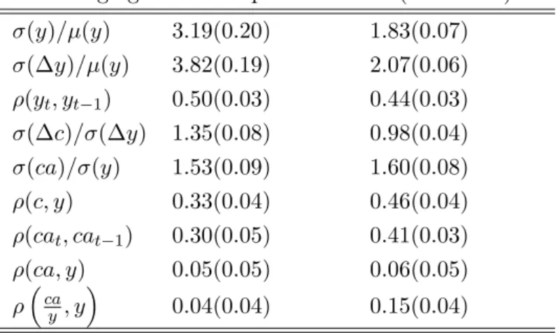
Table 2 and Table 3 report key statistics of emerging economies, and Table 4 and Table 5 report the same statistics for developed countries. To provide a comparison for the reader, we report the average values of these moments of both emerging countries and developed countries in Table 1. And we report both the results using a linear filter and that using a Hodrick-Prescott (HP) filter (with a smoothing parameter of 100) in the same table. For the variable growth (with a symbol ∆) the unfiltered series are used. The numbers in the parentheses are the GMM-corrected standard errors of the statistics across countries.9 Since our model setup is within the
permanent income framework in which agents make their consumption-saving decisions based on their perceived lifetime income, the low frequency components become important. Thus in this paper we focus primarily on the linear filter when we estimate the parameters and compare models with data; for comparison we also detrend the data using the Hodrick-Prescott filter.
[Insert Tables 1-5 Here]
We briefly list the facts we focus on. First, the correlation between the current account and net income is positive but small (and insignificant when detrended with the HP filter). Second, the relative volatility of the current account to net income is smaller in emerging countries than in developed economies, although the difference is not statistically significant when the series are detrended with the HP filter. Third, the persistence of the current account is smaller than that of net income, and less persistent in emerging economies. And fourth, the volatility of consumption growth relative to income growth is larger in emerging economies than in developed economies.
3
A Stylized Intertemporal Model of the Current Account
In this section we present a standard RE version of the ICA model and will discuss how to incorporate RB and RI into this stylized model in the next sections. Following common practice in the literature, we assume that the model economy is populated by a continuum of identical infinitely-lived consumers, and the only asset that is traded internationally is a risk-free bond.9The standard errors are computed under the assumption of independence across the countries. The standard
error ofσ(y)/µ(y) in the tables refers to the standard error ofσ(y) as the ratio ofµ(y). µ(y) is the average level of net income.
3.1 Model Setup
The RE ICA model, the small-open economy version of Hall’s permanent income model, can be formulated as max {ct} E0 [∞ ∑ t=0 βtu(ct) ] (1)
subject to the flow budget constraint
bt+1=Rbt+yt−ct, (2)
where u(ct) = −12(c−ct)2 is the utility function, c is the bliss point, ct is consumption, R is the exogenous and constant gross world interest rate, bt is the amount of the risk-free foreign bond held at the beginning of periodt, andytis net income in periodtand is defined as output less than investment and government spending. LetβR= 1; then this specification implies that optimal consumption is determined by permanent income:
ct= (R−1)st (3) where st=bt+ 1 R ∞ ∑ j=0 R−jEt[yt+j] (4)
is the expected present value of lifetime resources, consisting of financial wealth (the risk-free foreign bond) plus human wealth. As shown in Luo (2008) and Luo and Young (2009), in order to facilitate the introduction of robustness and rational inattention we reduce the above multivariate model with a general income process to the univariate model with iid innovations to permanent incomestthat can be solved in closed-form. Specifically, ifst is defined as a new state variable, we can reformulate the above PIH model as
v(s0) = max {ct,st+1}∞t=0 { E0 [∞ ∑ t=0 βtu(ct) ]} (5) subject to st+1 =Rst−ct+ζt+1, (6)
where the time (t+ 1) innovation to permanent income can be written as
ζt+1= 1 R ∞ ∑ j=t+1 ( 1 R )j−(t+1) (Et+1−Et) [yj] ; (7)
v(s0) is the consumer’s value function under RE. Under the RE hypothesis, this model with
quadratic utility leads to the well-known random walk result of Hall (1978),
∆ct= R−1 R (Et−Et−1) ∑∞ j=0 ( 1 R )j yt+j (8) = (R−1)ζt,
which relates the innovations in consumption to income shocks.10 In this case, the change in consumption depends neither on the past history of labor income nor on anticipated changes in labor income. In addition, the model specification also implies the certainty equivalence property holds, and thus uncertainty has no impact on optimal consumption.
Substituting (2) and (3) into the current account identity,
cat=bt+1−bt= (R−1)bt+yt−ct, (9) gives cat=− ∞ ∑ j=t+1 ( 1 R )j−t Et[∆yj], (10)
which means that the current account equals the present discounted value of future expected net income decreases. This expression also reflects the fact that consumers smooth income shocks by borrowing or lending in international financial markets. If income is expected to decline in the future, then the current account rises immediately as households import consumption goods; the opposite occurs if income is expected to rise in the future.
3.2 Model Predictions for Consumption and the Current Account
We close the model by specifying the stochastic process for net output. Specifically, we assume that the deviation of net output from its mean follows an AR(1) process
yt+1−y=ρ(yt−y) +εt+1, (11)
where ρ ∈ (0,1] is the persistence coefficient of output and εt+1 is an iid normal shock with
mean 0 and varianceω2.11 In this case, (7) implies thatζt+1= R1−ρεt+1 andst=bt+R1−ρyt. In the RE version of the ICA model, substituting (3) into the current account identity, (9), gives
cat= 1−ρ
R−ρyt, (12)
10
Note that under RE the expression of the change in individual consumption is the same as that of the change in aggregate consumption.
11
which means that given ρ and R, the current account inherits the properties of the stochastic process for net output (in particular, the persistence of net output). (12) also clearly shows that the value ofρ affects how output determines the behavior of the current account. Here we discuss two possibilities for the exogenous process of net output.12
Case 1 (0< ρ <1).
When ρ < 1, the shock is temporary and consumers adjust their optimal plans by only
consuming the annuity value of the increase in total income. In this case, the current account works as a shock absorber, and consumers borrow to finance negative income shocks and save in response to positive shocks. In other words, the current account in this case is procyclical:
∂cat
∂εt > 0, which means that the current account improves during expansions and deteriorates
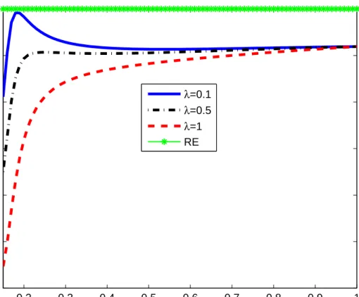
during recessions. The solid line in Figure 1 illustrates the impulse response of the current account to the income shock when R = 1.04 and ρ = 0.7. (We set R to be 1.04 throughout the paper; we treat it as a compromise of different asset returns in the economy.) Equation (12) also means that the contemporaneous correlation between the current account and income, corr (cat, yt), is 1. This model prediction contradicts the empirical evidence: in small open economies the correlation between the current account and net output is positive but close to 0. As reported in Panel A (HP filter) of Table 1, corr (cat, yt) = 0.04 (s.e. 0.04) in emerging countries and 0.06 (s.e. 0.05) in developed economies. Similarly, in Panel B (linear filter) of Table 1, corr (cat, yt) = 0.13 (s.e. 0.05) in emerging countries and 0.17 (s.e. 0.05) in developed economies. In other words, the model predicts too high a correlation between the current account and net output.
Equation (12) clearly shows that the volatility of the current account is less than that of income:
µ= sd (cat) sd (yt) =
1−ρ R−ρ <1,
where sd denotes standard deviation. Note that ∂µ∂ρ <0. Using the estimatedρreported in Panel A (HP filter) of Table 1 and assume that R = 1.04, the RE model predicts that µ = 0.926 in emerging countries andµ= 0.933 in developed countries. However, in the data (using HP filter) reported in Table 1, µ= 1.53 (s.e.0.09) in emerging countries, whereas µ= 1.60 (s.e. 0.08) in developed countries.13 In other words, given the estimated income processes, the model cannot correctly predict the magnitude of the relative volatility of the current account to net output emerging and developed economies.14
12
It should be understood that any nonstationarity in the data is driven by a time trend which we implicitly remove. The economy fits in the class of models that can be rendered stationary.
13
Given the estimatedρ using the linear filter reported in Panel B of Table 1, the RE model predicts that Λ = 0.83 in emerging countries and Λ = 0.84 in developed countries. However, in the data reported in Table 1, Λ = 0.8 (s.e.0.06) in emerging countries and Λ = 1.35 (s.e.0.06) in developed countries.
14
Equation (12) also implies that the persistence of the current account is the same as that of net output. However, in the data the current account is significantly less persistent than net output, and is less persistent in emerging economies than in developed economies. As shown in Panel B (linear filter) of Table 1, ρ(yt, yt−1) = 0.8 (s.e.0.02) and 0.79 (s.e. 0.02) in emerging
and developed countries, respectively, while the corresponding ρ(cat, cat−1) = 0.53 (s.e. 0.04)
and 0.71 (s.e.0.02).15
Furthermore, given the AR(1) income specification, the change in aggregate consumption is
∆ct=
R−1
R−ρεt, (13)
which means that consumption growth is white noise and the impulse response of consumption to the income shock is flat with an immediate upward jump in the initial period that persists indefinitely. (See the solid line in Figure 2.) However, as well documented in the consumption literature (Reis 2006), the impulse response of aggregate consumption to aggregate income takes ahump-shaped form, which means that aggregate consumption growth reacts to income shocks gradually.
In addition, the relative volatility of consumption growth and income growth can be written as µc = sd [∆ct] sd [∆yt] = R−1 R−ρ √ 1 +ρ 2 , (14)
where we use the facts thatζt= Rε−tρ, ∆ct= (R−1)ζt, and ∆yt=εt+ (ρ−1)1ε−t−ρ·1L, whereLis the lag operator. This expression is strictly increasing inρ, implying that consumption growth should be relatively more volatile in emerging economies (which is consistent with the data). However, given the values ofρ from Table 1, the volatility of consumption growth is much too low relative to net output. For example, if R = 1.04, the RE model predicts that the relative volatility of consumption growth to income growth in emerging and developed economies would be 0.28 and 0.24, respectively. In contrast, in the data, the correspondingµvalues are 1.35 and 0.98, respectively.16
Case 2 (ρ= 1).
Whenρ= 1,net output follows a unit root process and the current account becomes constant because consumers allocate all of the increase in net income to current consumption. Intuitively, when the income shocks are permanent, the best response is to adjust consumption plan perma-nently. This principle is called “finance temporary shocks, adjust to permanent shocks” in the literature. As a result, var [cat] = 0, which strongly contradicts the evidence that the current account is highly volatile in all small open economies.
15
As shown in Panel A of Table 1, using HP filter shows the same pattern.
16
In sum, comparing with the stylized facts reported in Table 1, it is clear that the stylized RE-ICA model with AR(1) income processes cannot explain the following key business cycle features in small open countries:
1. The contemporaneous correlation between the current account and net output is close to 0 in small open economies, and is slightly smaller in emerging markets.
2. The excess relative volatility of the current account to net output in emerging and devel-oped economies.
3. The persistence of the current account is smaller than that of net output, and it is smaller in emerging economies than in developed economies.
4. The hump-shaped impulse responses of consumption to income shocks.
5. The relative volatility of consumption growth to income growth is larger in emerging economies than in developed economies.
Finally, in the standard ICA model the current account is independent of the uncertainty in outputω2; that is, the amount of precautionary savings does not affect the current account surplus. The reason is that the LQ setup satisfies the certainty equivalence property, ruling out any response of saving to uncertainty. However, as shown in Ghosh and Ostry (1997), in the post-war quarterly data for the US, Japan, and the UK, the greater the uncertainty in income, the greater will be the incentive for precautionary saving and, ceteris paribus, the larger the current account surplus.17
4
Intertemporal Models of Current Account with Robustness
In this section, we introduce a concern for model uncertainty (robustness, RB) into the styl-ized intertemporal current account model (ICA) proposed in Section 3, and explore how this information imperfection affects the dynamics of consumption and the current account in the presence of income shocks.4.1 Optimal Consumption and the Current Account under Robustness Robust control emerged in the engineering literature in the 1970s and was introduced into economics and further developed by Hansen, Sargent, and others. A simple version of robust
17
Recent work examines the importance of precautionary savings for current account dynamics, including Sandri (2008), Mendoza, Quadrini, and R´ıos-Rull (2009), and Carroll and Jeanne (2009); such models are not analytically tractable and analysis is therefore somewhat less transparent.
optimal control considers the question of how to make decisions when the agent does not know the probability model that generates the data. In the ICA model present in Section 3, an agent with a preference for robustness considers a range of models surrounding the given approximating model, (6), and makes decisions that maximize expected utility given the worst possible model. Following Hansen and Sargent (2007a), a simple robustness version of the ICA model proposed in Section 3 can be written as
v(st) = max ct min νt { −1 2(c−ct) 2+β[ϑν2 t +Et[v(st+1)] ]} (15)
subject to the distorted transition equation (i.e., the worst-case model):
st+1=Rst−ct+ζt+1+ωζνt, (16)
where νt distorts the mean of the innovation and ϑ > 0 controls how bad the error can be.18 As shown in Hansen, Sargent, and Tallarini (1999) and Hansen and Sargent (2007a), this class of models can produce precautionary behavior while maintaining tractability within the LQ-Gaussian framework.
When output follows an AR(1) process, (11), solving this robust control problem and using the current account identity yields the following proposition:
Proposition 1 Under RB, the consumption function is
ct=
R−1
1−Σst− Σc
1−Σ, (17)
the mean of the worst-case shock is
ωζνt=
(R−1)Σ 1−Σ st−
Σ
1−Σc, (18)
the current account is
cat= 1−ρ R−ρyt+ Γst+ Σc 1−Σ, (19) and st ( =bt+ R1−ρyt ) is governed by st+1 =ρsst+ζt+1, (20)
where ζt+1=εt+1/(R−ρ), Σ =Rω2ζ/(2ϑ)>0 measures the degree of the preference of
robust-ness, Γ =−Σ(1R−−Σ1) <0, and ρs= 11−−RΣΣ ∈(0,1).
18Formally, this setup is a game between the decision-maker and a malevolent nature that chooses the distortion
processνt. ϑ≥0 is a penalty parameter that restricts attention to a limited class of distortion processes; it can
be mapped into an entropy condition that implies agents choose rules that are robust against processes which are close to the trusted one. In a later section we will apply an error detection approach to estimateϑin small open economies.
Proof. See Appendix 7.1.
The consumption function under RB, (17), shows that the preference for robustness, ϑ, affects the precautionary savings increment,−1−ΣΣc. The smaller the value of ϑ the larger the precautionary saving increment (Luo, Nie, and Young 2010 show that Σ < 1 is a necessary condition for nature to minimize utility). This expression also implies that the stronger the preference for robustness, the more consumption responds initially to changes in permanent income; that is, under RB consumption is more sensitive to unanticipated income shocks. This response is referred to as “making hay while the sun shines” in van der Ploeg (1993).
For the special case ρ= 1,
cat= Γst+ Σc
1−Σ, (21)
which clearly shows that the current account is countercyclical even if output follows a random walk: it improves during recessions and deteriorates during expansions. This model prediction matches the empirical evidence better than the standard ICA model.
4.1.1 Impulse Responses of the Current Account
When ρ ∈ (0,1), the effect of a change in net output on the current account is determined by the first two terms in (19), and the current account includes a unit root. Specifically,
∂cat ∂εt
= Γ + 1−ρ
R−ρ , (22)
which means that the current account will be procyclical if the preference for robustness is not sufficiently strong: Σ<Σ1 = 1−ρ R−ρ ( = 1− R−1 R−ρ ) . (23)
The dotted and dash-dotted lines in Figure 1 illustrate the impulse responses of the current account to the income shock when Σ = 0.5 and 0.95, respectively. For the special case that ρ = 1, introducing robustness generates countercyclical behavior of the current account as Σ>0.19
4.1.2 Volatility of the Current Account
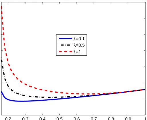
We now examine how RB affects the relative volatility of the current account to net income. Using (19), the relative volatility of the current account to net income can be written as
µ= sd (cat) sd (yt) = √{ (1−ρ2) [ 1−ρ 1 +ρ + Γ2 1−ρ2 s +2 (1−ρ) Γ 1−ρρs ]} /(R−ρ)2 <1, (24) 19
While the current account is not countercyclical with respect to net income, it is countercyclical with respect to GDP in many countries. Standard models attribute this countercyclicality to investment flows (Backus, Kehoe, and Kydland 1994). Our model offers an alternative interpretation.
where we use the facts that var (cat) = [ 1−ρ 1 +ρ + Γ2 1−ρ2 s + 2 (1−ρ) Γ 1−ρρs ] ω2 (R−ρ)2, (25) var (yt) = 1−ω2ρ2, var (st) = ω 2 (R−ρ)2(1−ρ2 s) , and cov (yt, st) = ω 2 (R−ρ)(1−ρρs).
Given R and ρ, (24) shows that µ is affected by the amount of robustness (Σ). Note that µ is not a monotonic function of Σ, as 1−Γ2ρ2
s in (24) is increasing with Σ and
2(1−ρ)Γ
1−ρρs in (24)
is decreasing with Σ. Given the complexity of this expression, we cannot obtain an explicit result about how RB affects µ. Figure 3 illustrates that how RB affects the relative volatility for different values of ρ. It is clear that µ is decreasing with Σ when Σ is relatively small and is increasing with Σ when Σ is large. The reason is that when Σ is large, the second term (the volatility term aboutst) in the bracket of (25) dominates the third term (the negative covariance term about st and yt) there. (Note that Γ< 0.) RB thus has a potential to make the model fit the data better along this dimension when Σ in small open economies is large enough and is larger in emerging economies than in developed economies. Note that we have shown in Section 3.2 that the stylized model cannot generate enough volatile current accounts, and the relative volatility of the current account to income is smaller in emerging economies than in developed economies.
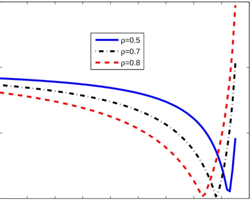
4.1.3 Persistence of the Current Account
The persistence of the current account is measured by its first autocorrelation. Using (19), the first autocorrelation of the current account,ρ(cat, cat−1), can be written as
ρ(cat, cat+1) = cov (cat, cat+1) √ var (cat) √ var (cat+1) = [ ρ(1−ρ) 1 +ρ + ρsΓ2 1−ρ2 s +(ρ+ρs) (1−ρ) Γ 1−ρρs ] / [ 1−ρ 1 +ρ + Γ2 1−ρ2 s +2 (1−ρ) Γ 1−ρρs ] , (26) which converges to ρ (the persistence of net income) as Σ goes to 0. Given the complexity of this expression, we cannot obtain an explicit result about how RB affectsρ(cat, cat+1). Figure
4 illustrates how RB affects the persistence of the current account for different values ofρ. It is clear thatρ(cat, cat+1) is decreasing with Σ. RB thus has a potential to make the model fit the
data better along this dimension. In addition, introducing RB can also explain thatρ(cat, cat+1)
is smaller in emerging countries than in developed countries if Σ is larger in emerging countries. Note that the standard RE-ICA model predicts that the current account and income have the same degree of persistence, which contradicts the evidence that the current account is signifi-cantly less persistent than income in small open economies and the persistence of net income is larger in emerging counties than in developed countries.
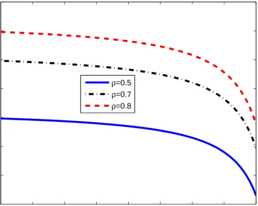
4.1.4 Correlation between the Current Account and Income
An alternative description of the comovement of the current account and income is the contem-poraneous correlation between the current account and income, corr (cat, yt). Under RB, the correlation can be written as:
corr (cat, yt) = ( Γ 1−ρρs + 1 1 +ρ ) / √ 1 (1 +ρ)2 + Γ2 (1−ρ2) (1−ρ2 s) + 2Γ (1 +ρ) (1−ρρs), (27) which reduces to 1 when Σ converges to 0. Figure 5 illustrates that how RB affects the correlation between the current account and net income for different values ofρ. It is clear that corr (cat, yt) is decreasing with Σ. (Note that in the figure we restrict the values of Σ to be less than 0.83 such that corr (cat, yt) is positive as generated in the data.) RB thus has the potential to align the model and the data more closely along this dimension. In addition, introducing RB can also account for the fact that corr (cat, yt) is smaller in emerging countries than in developed countries, provided Σ is larger in emerging countries.
4.1.5 Implications of Macroeconomic Uncertainty for the Current Account under
RB
Finally, the last term in (19) determines the effect of precautionary savings on the current account. It is clear that with the preference for robustness, the greater the uncertainty in net income, the greater the amount of precautionary saving, and the larger the current account surplus, as
∂cat
∂ω2ζ >0. (28)
This result is consistent with the empirical evidence that the current account and volatility are positively correlated (Ghosh and Ostry 1997). Note that the precautionary savings induced by a concern about robustness differs from the usual precautionary savings motive that emerges when labor income uncertainty interacts with the convexity of the marginal utility of consumption. This type of precautionary savings emerges because consumers want to save more as protection against model misspecification and thus occurs even in models with quadratic utility.
Having examined the implications of RB for the relative volatility and persistence of the current account, and the correlation between the current account and income, it is clear that RB has a potential to improve the model’s predictions on the joint dynamics of the current account and net income. A requirement for matching these facts is that the fear of misspecification is stronger in emerging economies. This requirement is obviously subject to empirical testing, so we will use the detection error approach of Hansen and Sargent (2007a) to estimate Σ for developed and emerging economies in a subsequent section.
4.1.6 Implication for Consumption Volatility
Although introducing robustness has a potential to improve the model’s predictions on the dynamics of the current account and precautionary savings, it worsens the model’s prediction for the joint dynamics of consumption and income. Given (17) and (20), the change in aggregate consumption can be written as
ct+1 =ρsct−
(1−R) Σc 1−Σ +
R−1
(1−Σ) (R−ρ)εt+1, (29) where ρs = 11−−RΣΣ and we use the fact that ζt+1 = εt+1/(R−ρ). Therefore, aggregate
con-sumption under RB follows an AR(1) process, which contradicts the evidence that in the data consumption reacts to income gradually and with delay. In other words, RB does not produce any propagation in consumption after an income shock. As emphasized in Sims (1998, 2003), VAR studies show that most cross-variable relationships among macroeconomic time series are smooth and delayed. Figure 2 illustrates the response of aggregate consumption growth to an aggregate income shockεt+1; comparing the solid line (RE) with the dash-dotted line, it is clear
that RB raises the sensitivity of consumption growth to unanticipated changes in aggregate income.
Furthermore, the relative volatility of consumption growth to income growth, µ, can be written as µc = sd [∆ct] sd [∆yt] = R−1 (1−Σ) (R−ρ) √ 1 +ρ 1 +ρs , (30)
where we also use the fact that ∆yt=εt+ (ρ−1)1ε−t−ρL1 .20 It is clear from (30) that RB increases the relative volatility via two channels: first, it strengthens the marginal propensity to consume out of permanent income
( R−1 1−Σ
)
; and second, it increases consumption volatility by reducing the persistence of permanent income measured by ρs: ∂ρ∂Σs <0. Furthermore, if Σ is larger in emerging economies, the RB-ICA model will predict that the relative volatility of consumption to income is greater in emerging economies than in developed economies.
4.2 Estimating the RB Parameter
In this section we use the procedure outlined Hansen, Sargent, and Tallarini (1999) and Hansen and Sargent (2007a) to estimate the RB parameter (ϑand Σ). Specifically, we estimate ϑ by using the notion of a model detection error probability that is based on a statistical theory of model selection (the approach will be precisely defined below). We can then infer what values of the RB parameter ϑ imply reasonable fears of model misspecification for empirically-plausible
20We use the relative volatility of consumption growth to income growth instead of that of consumption to
income to compare the implications of RE and RB models, as consumption follows a random walk under RE and the volatility of consumption is not well defined in this model.
approximating models. The model detection error probability is a measure of how far the distorted model can deviate from the approximating model without being discarded; low values for this probability mean that agents are unwilling to discard very many models (as they want errors to be rare), implying that the cloud of models surrounding the approximating model is large.
4.2.1 The Definition of the Model Detection Error Probability
Let modelA denote the approximating model and modelB be the distorted model. Define pA as pA= Prob ( log ( LA LB ) <0A ) , (31) where log ( LA LB )
is the log-likelihood ratio. When model A generates the data, pAmeasures the probability that a likelihood ratio test selects model B. In this case, we callpA the probability of the model detection error. Similarly, when model B generates the data, we can definepB as
pB= Prob ( log ( LA LB ) >0B ) . (32)
Following Hansen, Sargent, and Wang (2002) and Hansen and Sargent (2007b), the detection error probability,p, is defined as the average ofpAand pB:
p(ϑ) = 1
2(pA+pB), (33) where ϑ is the robustness parameter used to generate modelB. Given this definition, we can see that 1−pmeasures the probability that econometricians can distinguish the approximating model from the distorted model. Now we show how to compute the model detection error probability in the Robustness model.
4.2.2 Estimating the RB Parameter in the ICA Model
Under RB, assuming that the approximating model generates the data, the state, st, evolves according to the transition law
st+1 =Rst−ct+ζt+1,
= 1−RΣ 1−Σ st+
Σ
1−Σc+ζt+1. (34) In contrast, assuming that the distorted model generates the data, st evolves according to
st+1=Rst−ct+ζt+1+ωζνt,
=st+ζt+1. (35)
1. Simulate{st}Tt=0using (34) and (35) a large number of times. The number of periods used
in the simulation,T, is set to be the actual length of the data for each individual country. 2. Count the number of times that log
( LA LB ) <0A and log ( LA LB )
>0B are each satisfied. 3. Determine pA and pB as the fractions of realizations for which log
( LA LB ) <0A and log ( LA LB ) >0B, respectively.
In practice, given Σ, to simulate the {st}Tt=0 we need to know a) the volatility of ζt in (34) and (35), and b) the value of c. For a), we can compute it from sd (ζ) =
√
1−ρ2
R−ρ sd (y) where sd (y) is the standard deviation of net income. For b), we use the local coefficient of relative risk aversion γ =−uu′′′((cc))c = c¯−cc to recover the value ofc: c=
( 1 +1γ
)
E[c] whereE[c] is mean consumption. We choose γ = 2.
4.3 Estimation Results and Main Findings
After simulating the models and obtaining the detection error probability that circumscribes a neighborhood of models against which consumers want to assure robustness, we can find the values of ϑ and Σ associated with that probability. Having shown how the RB parameter is related to the model detection error probability, in this section we report the estimated values of the RB parameters by setting the model detection error probability to different targeted values. As a benchmark, we choose the RB parameter to match the model detection error probability of p= 0.1. That is, the probability that the agent can distinguish the approximating model from the distorted model is 0.9.
Tables 7 and 8 report the estimated values of RB parameter, Σ≡Rω2ζ/(2ϑ), as well as the associated model detection error, p, the autocorrelation coefficient of GDP, ρ, and the ratios of the standard deviation of real income and permanent income to the mean of real income (undetrended), σ(y)/µ(y) and σ(ζ)/µ(y), respectively.21 For simplicity here we only report the
results using the linear filter; using the HP filter generates similar patterns from the model. We use σ(y)/µ(y) to measure the relative volatility of fundamental uncertainty. Table 6 reports the averages over the emerging countries and that for the developed countries, respectively, and shows that on average:
1. Emerging countries face more volatile income processes than do developed countries. That is, macroeconomic uncertainty is higher in emerging countries.
2. After setting the detection error probabilityp(ϑ,Σ) to be the same in the two economies, the recovered Σ is larger in emerging countries.
21All tables in this paper are generated using the estimated parameters in the exogenous income processes. See
Therefore, the preference for robustness in emerging countries is stronger than in developed countries. The intuition is simple: agents in the emerging economy are more concerned about model misspecification because they face larger macroeconomic uncertainty and instability than those in developed countries. It is worth noting that a larger Σ does not necessarily imply a smaller value of ϑ since ωζ (i.e., σ(ζ)) can be different. As we have shown in Section 4.1, RB influences the countercyclical behavior of the current account and the relative volatility of consumption to income in the model through the interaction of ϑand ωζ in Σ instead of ϑ.
We first consider a comparison between the standard RE model and the RB model. In Tables 9-10, p is set to 0.1 such that Σ = 0.524 in emerging countries and 0.205 in developed countries. In this case the first three columns of the tables clearly show that RB can improve the model’s predictions along the following three dimensions: the contemporaneous correlation between the current account and net income, the persistence of the current account, and the relative volatility of consumption growth to income growth, but worsens the model prediction on the relative volatility of the current account to net income. Specifically, for emerging countries, given the estimated Σs RB reduces the correlation between the current account and net income from 1 to 0.62; reduces the first-order autocorrelation from 0.8 to 0.74; increases the relative volatility of consumption growth to income growth from 0.28 to 0.9; and reduces the relative volatility of the current account to income from 0.71 to 0.49. The intuition that RB reduces the volatility of the current account is that RB strengthens the response of consumption to income shock, and thus weakens current accounts effects of RB.
In Tables 11-12, we reduce the detection error probability to 0.01 and find that in this case RB can improve the model’s predictions along all the four dimensions including the relative volatility of the current account to net income. These quantitative results are consistent with the theoretical results we obtained in Section 4.1. The reason is that when the RB parameter is large enough, the second term in the bracket of (25) dominates the third term there, and thus increases the volatility of the current account. It is worth noting that p = 0.01 is an extremely low value and means that agents rarely make mistakes and thus can distinguish the models quite well.22 However, as shown in Tables 11-12, even for this extremely low detection error probability, the RB model still cannot generate the observed volatile current accounts, and cannot perform better than the RE model along this dimension. In the next section, we will show that introducing another informational friction, rational inattention, could help resolve this problem.
[Insert Tables 6-8 Here]
22
5
RB-RI Model
5.1 Optimal Consumption and the Current Account under RB and RI
5.1.1 Information-Processing Constraints
Under RI, consumers in the economy face both the usual flow budget constraint and information-processing constraint due to finite Shannon capacity first introduced by Sims (2003). As argued by Sims (2003, 2006), individuals with finite channel capacity cannot observe the state variables perfectly; consequently, they react to exogenous shocks incompletely and gradually. They need to choose the posterior distribution of the true state after observing the corresponding signal. This choice is in addition to the usual consumption choice that agents make in their utility maximization problem.23
Following Sims (2003), the consumer’s information-processing constraint can be character-ized by the following inequality:
H(st+1|It)− H(st+1|It+1)≤κ, (36)
where κ is the consumer’s channel capacity, H(st+1|It) denotes the entropy of the state prior to observing the new signal att+ 1,and H(st+1|It+1) is the entropy after observing the new
signal.24 The concept ofentropy is from information theory, and it characterizes the uncertainty in a random variable. The right-hand side of (36), being the reduction in entropy, measures the amount of information in the new signal received att+ 1. Hence, as a whole, (36) means that the reduction in the uncertainty about the state variable gained from observing a new signal is bounded from above by κ. Since the ex post distribution of st is a normal distribution, N(bst, σ2t
)
,(36) can be reduced to
log|ψt2| −log|σt2+1| ≤2κ (37) where sbt is the conditional mean of the true state, and σ2t+1 = var [st+1|It+1] and ψ2t = var [st+1|It] are the posterior variance and prior variance of the state variable, respectively. To obtain (37), we use the fact that the entropy of a Gaussian random variable is equal to half of its logarithm variance plus a constant term.
It is straightforward to show that in the univariate case (37) has a unique steady state σ2.25 In that steady state the consumer behaves as if observing a noisy measurement which
23More generally, agents choose the joint distribution of consumption and permanent income subject to
restric-tions about the transition from prior (the distribution before the current signal) to posterior (the distribution after the current signal).
24We regardκas a technological parameter. If the base for logarithms is 2, the unit used to measure information
flow is a ‘bit’, and if we use the natural logarithme, the unit is a ‘nat’. 1 nat is equal to log2e= 1.433 bits. 25Convergence requires thatκ >log (R)≈R−1; see Luo and Young (2009) for a discussion.
is s∗t+1 =st+1+ξt+1, where ξt+1 is the endogenous noise and its variance α2t = var [ξt+1|It] is determined by the usual updating formula of the variance of a Gaussian distribution based on a linear observation:
σt2+1 =ψ2t −ψ2t(ψt2+α2t)−1ψ2t. (38)
Note that in the steady state σ2 = ψ2 −ψ2(ψ2+α2)−1ψ2, which can be solved as α2 = [(
σ2)−1−(ψ2)−1 ]−1
. Note that (38) implies that in the steady stateσ2= ( 1 R−ρ )2 ω2 exp(2κ)−R2.and α2 = var [ξt+1] = [ ω2/(R−ρ)2+R2σ2]σ2 ω2/(R−ρ)2+(R2−1)σ2.
5.1.2 Incorporating RI into the RB Model
We now incorporate RI into the RB model and examine how the combination of the two types of information imperfections affect the joint dynamics of consumption, the current account, and income.26 A key assumption in the RB-RI model is that we assume that the consumer not only has doubts about the process for the shock to permanent income ζt+1, but also distrusts his
regular Kalman filter hitting the endogenous noise (ξt+1) and updating the estimated state. As
a result, our agents have an additional dimension along which they desire robustness.
Specifically, the regular RI-induced Kalman filter equation updating the estimated state (bst), b
st+1 = (1−θ) (Rbst−ct) +θ(st+1+ξt+1), (39)
where bst = E[st|It] is the conditional mean of st, ξt+1 is the iid endogenous noise with α2 =
var [ξt+1] = [
ω2/(R−ρ)2+R2σ2]σ2
ω2/(R−ρ)2+(R2−1)σ2, θ = σ
2/α2 = 1−1/exp(2κ) ∈ [0,1] is the constant optimal
weight on any new observation, ands0 ∼N
( b s0, σ2
)
is fixed.27 Combining (39) with the budget constraint, st+1 =Rst−ct+ζt+1, yields the following equation governing the dynamics of the
perceived statebst that matters in agents’ decision problems: b
st+1=Rbst−ct+ηt+1, (40)
where
ηt+1 =θR(st−bst) +θ(ζt+1+ξt+1) (41)
is the innovation to the mean of the distribution of perceived permanent income,
st−bst= (1−θ)ζt 1−(1−θ)R·L− θξt 1−(1−θ)R·L. (42) 26
The RB-RI model proposed in this paper encompasses the hidden state model discussed in Hansen, Sargent, and Wang (2002) and Hansen and Sargent (2007b); the main difference is that none of the states in the RB-RI model are perfectly observable (or controllable).
27
θmeasures how much new information is transmitted each period or, equivalently, how much uncertainty is removed upon the receipt of a new signal.
and Et[ηt+1] = 0. To introduce robustness into the RI model, we assume that the agent thinks
that (40) is the approximating model for the true model that governs the data but that he cannot specify. Following Hansen and Sargent (2007a), we surround (40) with a set of alternative models to represent his preference for robustness:
b
st+1 =Rsbt−ct+ωηνt+ηt+1. (43)
Under RI the innovation ηt+1, (41), that the agent distrusts is composed of two MA(∞)
pro-cesses and includes the entire history of the exogenous income shock and the endogenous noise,
{ζt+1, ζt,· · ·, ζ0;ξt+1, ξt,· · ·, ξ0}.
The optimizing problem for this RB-RI model is formulated as
b v(bst) = max ct min νt { −1 2(ct−c) 2+βE t [ ϑνt2+bv(bst+1) ]} , (44)
subject to (43)-(42). (44) is a standard dynamic programming problem. The following proposi-tion summarizes the soluproposi-tion to the RB-RI model.
Proposition 2 Given ϑand θ, the consumption function under RB and RI is
ct=
R−1
1−Σbst− Σc
1−Σ, (45)
the mean of the worst-case shock is
ωηνt= (R−1)Σ 1−Σ bst− Σ 1−Σc, (46) and bst is governed by b st+1=ρssbt+ηt+1. (47) where ρs = 11−−RΣΣ ∈(0,1), Σ =Rωη2/(2ϑ)>0, (48) ω2η = var [ηt+1] = θ 1−(1−θ)R2ω 2 ζ. (49)
It is clear from (45)-(49) that RB and RI affect the consumption function via two channels in the model: (1) the marginal propensity to consume (MPC) out of the perceived state
( R−1 1−Σ
) and (2) the dynamics of the perceived state (bst). Given bst, stronger degrees of RI and RB increase the value of Σ, which increases the MPC.
Before proceeding, we want to draw a distinction between the model proposed above and similar ones used in Luo and Young (2009) and Luo, Nie, and Young (2010). In those other papers, agents were assumed to trust the Kalman filter they use to process information, meaning
that decisions were only robust to misspecification of the income process. In that model Σ was independent of θ, and for the questions at hand here the resulting values were too small. By adding the additional concern for robustness developed here, we are able to strengthen the effects of robustness on decisions. In addition, our setup here is arguably more consistent with the underlying primitive structure of ambiguity that gives rise to robust decision-making (Gilboa and Schmeidler 1989).
5.1.3 The Joint Dynamics of Consumption, the Current Account, and Net Income
under RB-RI
Furthermore, in the RB-RI model individual dynamics are not identical to aggregate dynamics. Combining (45) with (43) yields the change in individual consumption in the RI-RB economy:
∆ct= (1−R) Σ 1−Σ (ct−1−c) + R−1 1−Σ ( θζt 1−(1−θ)R·L+θ ( ξt− θRξt−1 1−(1−θ)R·L )) , where L is the lag operator and we assume that (1− θ)R < 1.28 This expression shows that consumption growth is a weighted average of all past permanent income and noise shocks. Since this expression permits exact aggregation, we can obtain the change in aggregate consumption as ∆ct= (1−R) Σ 1−Σ (ct−1−c) + R−1 1−Σ ( θζt 1−(1−θ)R·L +θ ( ξtEi[ξt]− θRξt−1 1−(1−θ)R·L )) , (50) where idenotes a particular individual, Ei[·] is the population average, and ξ
t=Ei[ξt] is the common noise.29 This expression shows that even if every consumer only faces the common shock ζ, the RI economy still has heterogeneity since each consumer faces the idiosyncratic noise induced by finite channel capacity. As argued in Sims (2003), although the randomness in an individual’s response to aggregate shocks will be idiosyncratic because it arises from the individual’s own information-processing constraint, there is likely a significant common compo-nent. The intuition is that people’s needs for coding macroeconomic information efficiently are similar, so they rely on common sources of coded information. Therefore, the common term of the idiosyncratic error,ξt, lies between 0 and the part of the idiosyncratic error,ξt, caused by the common shock to permanent income, ζt. Formally, assume that ξt consists of two independent noises: ξt=ξt+ξti, where ξt=Ei[ξt] and ξit are the common and idiosyncratic components of the error generated byζt, respectively. A single parameter,
λ= var
[ ξt]
var [ξt] ∈[0,1],
28
This assumption is generally innocuous, since it is only violated ifθ is very close to 0.
can be used to measure the common source of coded information on the aggregate component (or the relative importance ofξtvs. ξt).30 Figure 2 also shows how RI can help generate the smooth and hump-shaped impulse response of consumption to the income shock, which, as argued in Sims (1998, 2003), fits the VAR evidence better.
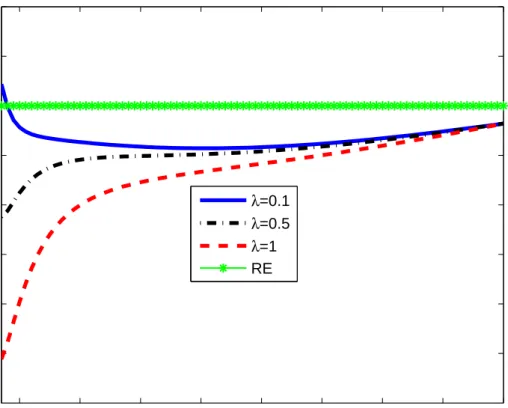
In a recent paper, Angeletos and La’O (2009) show how dispersed information about the underlying aggregate productivity shock contributes to significant noise in the business cycle and helps explain cyclical variations in observed Solow residuals and labor wedges in the RBC setting. In contrast, Lorenzoni (2009) examines how demand shocks, defined as noisy news about future aggregate productivity, contribute to business cycles fluctuations in a new Keynesian model. In the next section, after calibrating the RB parameter we also show that the common noise due to finite capacity can simultaneously increase the relative volatility of consumption growth and income growth and reduce the contemporaneous correlation between the current account and income, which makes the RB-RI model fit the data better.
Substituting (45) into the current account identity, the current account in the RB-RI model economy can be written as
cat= 1−ρ R−ρyt− Σ (R−1) 1−Σ st+ R−1 1−Σ(st−bst) + Σ 1−Σc, (51) where st−bst= (1−θ)ζt 1−(1−θ)R·L − θEi[ξt] 1−(1−θ)R·L (52) is the error in estimating st. It is clear that when θ = 1, (51) reduces to (19) in Section 4.1. The expression for the current account, (51), clearly shows that in the RB-RI model the current account is determined by four factors:
1. The income process,−Rρ−ρ∆yt. Holding other factors constant, the current account dete-riorates in response to a positive shock to income.
2. The overreaction in consumption due to the preference for robustness, −Σ(1R−−Σ1)st. This expression means that the stronger the preference for robustness, the more countercyclical the current account is. Under robustness, consumption is more sensitive to the unantici-pated income shock, and thus the increase in consumption is larger than that of income itself; consequently, the current account deteriorates.
3. The forecast error term due to rational inattention, R1−−Σ1(st−bst). Consumers with finite capacity cannot observe the state perfectly, and thus adjust optimal consumption gradu-ally and with delay. For a positive income shock, a gradual adjustment in consumption improves the current account.
30It is worth noting that the special case thatλ= 1 can be viewed as a representative-agent model in which
4. The precautionary savings term, 1Σ−cΣ. The precautionary saving premium due to the fear of model misspecification induces a bias toward current account surplus.
Figure 1 also plots the impulse response of the current account to the income shock when Σ = 0.95 and θ= 80%. It clearly shows that the current account also responds to the income shock smoothly and gradually, which can better fit the VAR evidence that most cross-variable relationship among macroeconomic time series are smooth and delayed. Using (51) it is straight-forward to show that the current account is procyclical if the following inequality is satisfied:
Σ<1−θR−1
R−ρ. (53)
5.1.4 Volatility of the Current Account
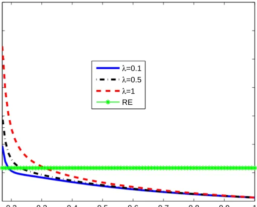
Under RB-RI, using (51), the relative volatility of the current account and net income can be written as µ= sd (cat) sd (yt) = √ 1−ρ2 R−ρ v u u u t 1−ρ 1+ρ+ Γ2 1−ρ2 s + ( R−1 1−Σ )2[(1−θ)2 1−ρ2 θ +1θλ−ρ22 θ 1 (1/(1−θ)−R2) ] +2(11−−ρρρ)Γ s + ( R−1 1−Σ ) 2(1−ρ)(1−θ) 1−ρρθ + ( R−1 1−Σ ) 2Γ(1−θ) 1−ρsρθ . (54)
Given the complexity of this expression, we cannot obtain an explicit result about how the interactions of RI and RB affect the relative volatility. As in the RB case, we thus use a figure to illustrate how RB and RI affect the relative volatility. Figure 6 illustrates the effects of RI on the relative volatility when Rω2ζ/(2ϑ) = 0.5 and ρ = 0.8. Note that in the RB-RI case, Σ = Rωη2/(2ϑ) = 1−(1−θθ)R2Rω2ζ/(2ϑ) as ωη2 = 1−(1−θθ)R2ωζ2. It is clear from the figure
that given the aggregation factor (λ), the relative volatility is decreasing with the degree of attention (θ); given θ, the relative volatility is increasing with λ. The intuition for the first result is that holding the aggregation factor fixed (i.e., given the impact of the common noise), reducingθincreases the smoothness of aggregate consumption, and thus increases the volatility of the current account. The intuition for the second result is that holding θ fixed, increasing λstrengthens the importance of the common noise, which leads to more volatile consumption and current accounts. Therefore, RI measured byθ and λhas the potential to make the model fit the data better along this dimension. In the next section, we will examine how RI and RB improve the model’s quantitative predictions.