A SCALABLE FRAMEWORK FOR PARALLELIZING SAMPLING-BASED MOTION PLANNING ALGORITHMS
A Dissertation by
SAMSON ADE JACOBS
Submitted to the Office of Graduate and Professional Studies of Texas A&M University
in partial fulfillment of the requirements for the degree of DOCTOR OF PHILOSOPHY
Chair of Committee, Nancy M. Amato Committee Members, Lawrence Rauchwerger
Valerie Taylor Jim Morel
Head of Department, Nancy M. Amato
May 2014
Major Subject: Computer Science
ABSTRACT
Motion planning is defined as the problem of finding a valid path taking a robot (or any movable object) from a given start configuration to a goal configuration in an environment. While motion planning has its roots in robotics, it now finds application in many other areas of scientic computing such as protein folding, drug design, virtual prototyping, computer-aided design (CAD), and computer animation. These new areas test the limits of the best sequential planners available, motivating the need for methods that can exploit parallel processing.
This dissertation focuses on the design and implementation of a generic and scal-able framework for parallelizing motion planning algorithms. In particular, we focus on sampling-based motion planning algorithms which are considered to be the state-of-the-art. Our work covers the two broad classes of sampling-based motion planning algorithms — the graph-based and the tree-based methods. Central to our approach is the subdivision of the planning space into regions. These regions represent sub-problems that can be processed in parallel. Solutions to the sub-sub-problems are later combined to form a solution to the entire problem. By subdividing the planning space and restricting the locality of connection attempts to adjacent regions, we re-duce the work and inter-processor communication associated with nearest neighbor calculation, a critical bottleneck for scalability in existing parallel motion planning methods. We also describe how load balancing strategies can be applied in complex environments. We present experimental results that scale to thousands of processors on different massively parallel machines for a range of motion planning problems.
DEDICATION
To my beloved wife, Wuraola; love is our greatest asset, the future is nothing to fear. To our two adorable daughters, Molayo and Moyo; with all thy getting, get wisdom.
ACKNOWLEDGEMENTS
I am indebted to a number of people for their support in the course of my PhD program.
First and foremost, my advisor and mentor, Prof. Nancy M. Amato, for her continual support and sometime demanding request which has made me both a better researcher and a leader. Her passion for excellence is one thing I will cherish for years to come.
I would like to thank my committee members, Prof. Lawrence Rauchwerger, Prof. Valerie Taylor, and Prof. Jim Morel, for their useful suggestions and guidance. I would like to thank faculty, staff, postdocs, alumni, and current students of Parasol Lab who in one way or other have made contributions to the work presented in this dissertation. Worth mentioning here are the following individuals: Prof. Jennifer Welch, Kay Jones, David Ramirez, Dr. Shawna Thomas, Dr. Roger Pearce, Dr. Gabriel Tanase, Dr. Timmie Smith, Dr. Nathan Thomas, Harshvardan, Adam Fidel, Antal Buss, Ioannis Papadopoulos, Shishir Sharma, Bryan Boyd, Jory Denny, Kasra Manavi, Troy McMahon, Chinwe Ekenna, Cindy Yeh, Andy Giese, and Daniel Tomkins.
I acknowledge the work of undergraduate students whom I have had the privilege to mentor, in particular, Juan Burgos, Cesar Rodriguez both from Texas A&M Uni-versity, Dezshaun Meeks from Praire View A&M UniUni-versity, and Nicholas Stradford from University of North Texas. I am grateful to them for their contributions to this work.
Lastly, I would like to thank my family and friends for their love, patience, and support.
TABLE OF CONTENTS Page ABSTRACT . . . ii DEDICATION . . . iii ACKNOWLEDGEMENTS . . . iv TABLE OF CONTENTS . . . v
LIST OF FIGURES . . . viii
1. INTRODUCTION . . . 1
1.1 Research Contributions . . . 5
1.2 Outline . . . 6
2. PRELIMINARIES AND RELATED WORK . . . 7
2.1 Preliminaries . . . 7
2.1.1 Motion Planning . . . 7
2.1.2 Sampling-Based Motion Planning . . . 7
2.2 Related Work . . . 10
2.2.1 Parallel Sampling-Based Motion Planning . . . 10
2.2.2 Space Subdivision . . . 16
2.2.3 Load Balancing Techniques . . . 17
3. STRATEGY FOR PARALLELIZING SAMPLING-BASED MOTION PLAN-NING ALGORITHMS . . . 20
3.1 Strategy Overview . . . 20
3.2 STAPL Framework . . . 22
4. GRAPH-BASED PARALLEL MOTION PLANNING . . . 26
4.1 Space Subdivision and Region Graph Construction . . . 26
4.2 Constructing Regional Roadmaps . . . 27
4.3 Connecting Regional Roadmaps . . . 29
4.4 Algorithm Analysis . . . 30
4.5 Experimental Evaluation . . . 32
4.5.1 Algorithms . . . 32
4.5.2 Machine Architectures . . . 32
4.5.3 Motion Planning Problems . . . 33
5. TREE-BASED PARALLEL MOTION PLANNING . . . 41
5.1 Space Subdivision and Region Graph Construction . . . 41
5.2 Constructing Regional Subtrees . . . 42
5.3 Connecting Regional Subtrees . . . 42
5.4 Algorithm Analysis . . . 43
5.5 Experimental Evaluation . . . 46
5.5.1 Bulk Synchronous Distributed RRT . . . 46
5.5.2 Parallelizing Nearest Neighbor Search . . . 47
5.5.3 Machine Architecture . . . 48
5.5.4 Motion Planning Problems . . . 50
5.5.5 Experimental Results . . . 50
6. RADIAL BLIND RRT . . . 58
6.1 Blind RRT . . . 58
6.1.1 Algorithm . . . 59
6.1.2 Probabilistic Completeness . . . 61
6.2 An Improved Radial RRT using Blind RRT . . . 62
6.2.1 Algorithm . . . 62 6.2.2 Probabilistic Completeness . . . 65 6.2.3 Algorithm Analysis . . . 67 6.3 Experimental Evaluation . . . 69 6.3.1 Experimental Setup . . . 69 6.3.2 Map Coverage . . . 71 6.3.3 Parallel Performance . . . 72
7. USING LOAD BALANCING TO SCALABLY PARALLELIZE SAMPLING-BASED MOTION PLANNING ALGORITHMS . . . 74
7.1 Basic Load Balancing Techniques . . . 75
7.2 Load Balancing for PRM . . . 77
7.3 Load Balancing for RRT . . . 79
7.4 Implementation in STAPL . . . 81
7.5 Experimental Evaluation . . . 83
7.5.1 Setup . . . 83
7.5.2 Parametrically Imbalanced Environment . . . 84
7.5.3 Experimental Results . . . 90
8. ROADMAP QUALITY ANALYSIS . . . 95
8.1 Evaluation Metrics . . . 95
8.1.1 Edge Metrics . . . 95
8.1.2 Coverage and Connectivity Metrics . . . 97
8.1.3 Query Processing and Path Length . . . 99
8.1.4 Structural Metrics . . . 99
8.2 Roadmap Graph Properties . . . 100
8.3.1 Setup . . . 102
8.3.2 Experimental Results . . . 102
8.4 Heterogeneous Environment: A Natural Fit for Spatial Subdivision and Parallelism . . . 109
8.4.1 Adaptive Sampling and Connection . . . 112
8.4.2 Experimental Results . . . 113
9. CONCLUSION . . . 118
LIST OF FIGURES
FIGURE Page
1.1 Planning space subdivision strategies: (a) uniform subdivision and (b)
ra-dial subdivision . . . 4
2.1 An illustration of PRM . . . 9
2.2 An illustration of RRT . . . 11
2.3 An illustration of SRT . . . 16
3.1 Types of subdivision: (a) uniform (b) radial (c) adaptive . . . 23
3.2 STAPL software architecture. . . 25
4.1 Space subdivision: (a) A 2D environment subdivided into 9 regions, (b) region graph - the 9 vertices represent each of the 9 regions with corre-sponding color, edges encode the adjacency information between regions. . 28
4.2 Environments studied for graph-based method . . . 34
4.3 Comparison of our proposed method (pSBMP-PRM and pSBMP-RRT) to two existing approaches: pPRM and pSRT . . . 35
4.4 Results from three different motion planning problems on Linux cluster using pSMBP-PRM and pSMBP-RRT methods . . . 38
4.5 Results from varying input size for the articulated linkage robot in a clut-tered environment using pSMBP-PRM method . . . 39
4.6 Higher processor counts on Cray XE6 petascale machine . . . 40
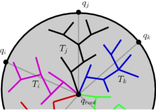
5.1 Example of radial subdivision for a 2D Cspace. Each process concur-rently builds a branch (using sequential RRT) rooted atqr and biased toward a target qi (e.g., qn for the black process). . . 42
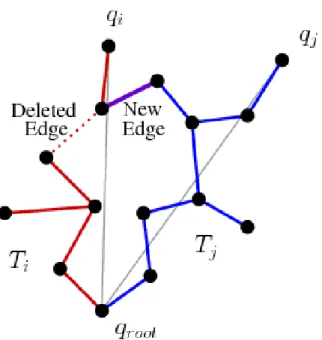
5.2 Tree pruning example, the new edge (purple) between the red and blue branches causes a cycle in the red branch, the dashed edge is
identified for removal. . . 44
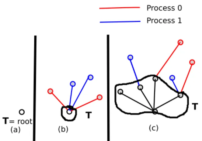
5.3 Bulk synchronous distributed RRT. (a) T is initialized to root, (b) The first iteration withm=2, (c) The second iteration where globally communicated data is shown in black. . . 48
5.4 Environments studied for tree-based method . . . 51
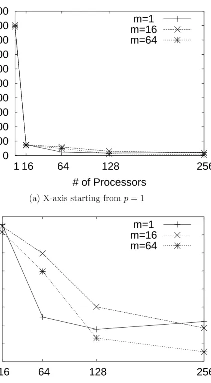
5.5 Effect of varying m in the bulk synchronous distributed RRT. . . 53
5.6 Radial subdivision distributed RRT performance on Linux cluster. . . 54
5.7 Distributed RRT performance on Cray XE6 machine. . . 56
5.8 Radial RRT performance results for grid environment on Cray XE6 machine . . . 57
5.9 Radial RRT performance results for stripline environment on Linux cluster . . . 57
6.1 RRT expands greedily up to ∆q, qrand, or an obstacle is hit (a) Blind RRT Expand always expands up to ∆q distance or qrand while also retaining either all free witnesses (b) or only the first free witness (c) to return a set of expansion nodes Qnew. . . 61
6.2 (a) An example environment with four regions, represented by their points (blue) on the outer circle. (b) Radial Blind RRT concurrently expanding in the four regions ignoring obstacles as it goes. (c) Radial Blind RRT concurrently and locally removes invalid nodes of the tree and connects CCs within each region (new edges emphasized in ma-genta). (d) Radial Blind RRT connectsCCsbetween regions yielding a final tree. . . 66
6.3 Example of Radial RRT not being able to solve an example query. . . 66
6.4 Motion planning problems. . . 68
6.5 Comparing coverage after performing RRT, Radial RRT, and Radial Blind RRT. All results are normalized to RRT. . . 70
7.1 Roadmap graph node distribution (a) before rebalancing: majority of nodes are present on two processors (green and brown color) (b) after rebalancing: almost even distribution of nodes. . . 74 7.2 Regular subdivision method for parallel PRM. . . 76 7.3 The fundamental migrate primitive, redistribution of a container based
on a view and rebalancing a view based on weights. . . 81 7.4 Customizable scheduling scheme for a call to a parallel algorithm. . . 83 7.5 Imbalanced cube environment . . . 84 7.6 Subdivision of imbalanced cube environment . . . 85 7.7 In a 3x3 spatial decomposition, the (a) model’s estimation of the
vol-ume of free space and (b) the number of roadmap nodes sampled per region in a test run. . . 87 7.8 In a 9x9 spatial decomposition, the (a) model’s estimation of the
vol-ume of free space and (b) the number of roadmap nodes sampled per region in a test run. . . 88 7.9 Experimental validation of measure of load imbalance in model
envi-ronment. (α = 2, β = 4 andRx= 256, Ry = 1) . . . 88 7.10 Experimental validation of potential improvement in model
environ-ment. (α= 2, β= 4 and Rx = 256, Ry = 1) . . . 89 7.11 Evaluation of (a) execution time and (b) coefficient of variation and
(c) load distribution for PRM on Hopper. . . 91 7.12 Evaluation of computing roadmap in the walls environment for a rigid
body robot on Hopper . . . 91 7.13 Execution time for PRM with various load balancing strategies in (a)
walls (b) walls-45 (c) and free environment. . . 92 7.14 Breakdown of the amount of tasks stolen vs. executed locally for PRM
on (a) 96 and (b) 768 cores on Hopper. . . 93 7.15 Breakdown of (a) the various phases of PRM (b) and the effect of load
balancing on remote accesses. . . 94 7.16 Execution time for RRT with various load balancing strategies in (a)
8.1 Impact of space subdivision on graph structure: For a given query point (red), 3-nearest neighbors are shown in green. Selected
neigh-bors differ as a result of space subdivision. . . 102
8.2 Environments . . . 103
8.3 Quality evaluation in free environment . . . 105
8.4 Relationship between diameter and average shortest paths . . . 106
8.5 Page (vertex) rank for different region subdivision . . . 107
8.6 Page (vertex) rank distributions for 1 and 4 regions . . . 108
8.7 Quality evaluation in 3D clutter environment . . . 109
8.8 Quality evaluation in 2D clutter environment . . . 110
8.9 Paths for (a) sequential planner, and (b-d) parallel planner at different processor counts . . . 110
8.10 Roadmap and paths for (a) sequential planner, and (b-d) parallel plan-ner at different processor counts . . . 111
8.11 Quality evaluation in maze environment . . . 111
8.12 Heterogeneous environments . . . 113
8.13 Region classification : number of regions per sampler for both 2D and 3D heterogenous environments . . . 114
8.14 Quality evaluation in 2D heterogenous environment . . . 116
1. INTRODUCTION
This dissertation presents a scalable framework for parallelizing sampling-based motion planning algorithms. Motion planning is defined as the problem of finding a valid path taking a robot (or any movable object) from a given start configuration to a goal configuration in an environment. While motion planning has its roots in robotics, it now finds applications in other areas of scientific computing including protein folding [1, 2, 3], minimally-invasive surgical planning [4], and drug design [5, 6, 7, 8], and computer-aided design [9, 10, 11, 12]. These new application areas are known to test the limit and capability of existing sequential motion planners [13]. Due to the infeasibility of exact motion planning [14, 15], sampling-based methods [15] are now the state-of-the-art for solving motion planning problems. Sampling-based approaches are efficient and can be applied to problems with many degrees of freedom (e.g., robotic manipulators with many links or proteins with many amino acids). While not guaranteed to find a solution, sampling-based methods are known to be probabilistically complete, meaning that the probability of finding a solution, given one exists, increases with the number of samples generated [16]. Sampling-based motion planning algorithms have been highly successful at solving previously unsolved problems [4, 15], and much research has focused on developing more so-phisticated variants of them [4, 15].
Sequential sampling-based motion planning algorithms still require substantial resources in time and hardware to solve computationally intensive applications. For example, modeling the motion of a small protein using sequential sampling-based motion planning techniques can take days on a typical desktop machine [17]. This time increases to several weeks if more accurate energy calculations are used or if
larger proteins are studied. Hence, it is practically infeasible to study larger pro-teins or to significantly increase the detail and accuracy at which their motions are modeled. To address this problem, researchers have turned to parallel pro-cessing as an alternative option to explore. For many application areas, parallel processing offers the advantage of not only reducing computation time, but also im-proving the solution quality and enabling larger problems to be solved than were feasible before. Although there has been some research in parallel motion planning [18, 19, 20, 21, 17, 22, 23, 24, 25, 26, 13], no scalable solution has been proposed.
This research proposes a new framework for parallelizing sampling-based motion planning algorithms. Central to our proposed framework [27, 28, 29] is the novel subdivision of the planning space into regions and an abstraction that represents the spatial relationship between the regions called a region graph R(V, E). The vertices, V, of the region graph represent the regions and the edges, E, represent the adjacencies between regions. The regions represent subproblems that can be processed independently (and in parallel). The task or subproblem associated with each region is to build a roadmap (graph or tree) that encodes representative paths approximating the topology of the planning space of the associated region. The regional roadmaps are later combined to obtain a roadmap for the entire space. This merging of regional roadmaps is facilitated using the region graph. In particular, the
region graph is the enabling infrastructure facilitating the process of connecting the regional roadmaps as its edges identify adjacent regions between which connections are attempted.
By subdividing the planning space and restricting the locality of connection at-tempts to adjacent regions, we reduce the work and inter-processor communication associated with nearest neighbor calculation, a critical bottleneck in the scalability of existing parallel motion planning methods [30, 31, 23, 24]. While our framework
employs the standard sequential planners (e.g., the probabilistic roadmap method (PRM)[16] or rapidly-exploring random tree (RRT)[32]) as underlying motion plan-ning algorithms, the resulting roadmap may be structurally different than would result if one of them were applied to the problem as a whole. Hence, we carried out an experimental evaluation of our algorithms to study both the structural difference and its impact on the solution of the motion planning problems.
In addition, we address the problem of load balancing [33] in complex planning spaces. For most complex planning spaces, as the granularity of the subdivision increases, the heterogeneity of the regions will increase, leading to an increase in load imbalance because the cost of planning depends on the complexity of the region. To address the load imbalance, we apply standard load balancing techniques based on data-structure redistribution and work stealing and show the effectiveness of the two techniques at combating load balancing issues that arise at scale.
Unlike other previous and related work, our work covers the two broad classes of sampling-based motion planners: graph-based (e.g., the probabilistic roadmap method (PRM)[16]) and tree-based (e.g., rapidly-exploring random tree (RRT)[32]) methods. We explored different planning space subdivision approaches suitable for the two sampling-based motion planning broad classes: a uniform mesh-like subdi-vision for graph-based (see Figure 1.1(a)) and radial subdisubdi-vision (see Figure 1.1(b)) for tree-based. We provide both theoretical and empirical proof of scalable and su-perior performance compared to previous methods. We present experimental results obtained from our studies of a wide range of motion planning problems utilizing different parallel architectures; ranging from small-scale linux clusters to an IBM Power5+ machine to a Cray XE6 petascale machine.
(a)
(b)
Figure 1.1: Planning space subdivision strategies: (a) uniform subdivision and (b) radial subdivision
1.1 Research Contributions
The key contributions of this dissertation can be summarized as follows:
The first reported work in parallel sampling-based motion planning based on spatial subdivision of the configuration space (Cspace). Our proposed framework is compatible with any sampling-based algorithm, including both graph-based methods, e.g., the Probablistic Roadmap (PRM) and the tree-based methods, e.g., Rapidly-exploring Random Trees (RRT).
A novel radial subdivision ofCspace suitable for tree-based planners that allows the computation to be distributed efficiently.
A novel motion planning algorithm, Blind RRT capable of exploring the free space (Cf ree) regardless of the obstacle space (Cobstacle) to Cf ree ratio. Blind RRT provides both scalability and probablistic completeness for motion plan-ning.
Experimental results demonstrate we achieve better and more scalable per-formance on thousands of processors than previous parallel sampling-based planners. Application of load balancing techniques based on data-structure redistribution and work-stealing to achieve scalability across different motion planning problems.
Much of this research has been published [34, 27, 28, 29, 35, 33]. A poster [27] and a paper [28] describing the parallelization of graph-based motion planning algo-rithms were presented at the 2011ACM/Microsoft Research Student Research Poster Competition at Supercomputing Conference (SC) and the 2012 IEEE International Conference on Robotics and Automation (ICRA), respectively. Radial subdivision
for RRT [29] and blind RRT [35] were published at ICRA 2013 and the IEEE/RSJ International Conference on Robotics and Systems (IROS) 2013, respectively. Our work on using load balancing techniques for complex motion planning problems [33] will be presented at IEEE International Parallel and Distributed Processing Sympo-sium (IPDPS) in 2014.
1.2 Outline
The rest of this dissertation is organized as follows. We provide an overview of sampling-based motion planning and a survey of related work on parallel motion planning in Chapter 2. In Chapter 3, we discuss the overview of the scalable frame-work for parallelizing sampling-based motion planning algorithms. In Chapter 4 and Chapter 5, we focus on the specifics of our framework for parallelizing the graph-based and the tree-graph-based motion planning algorithms, respectively. In Chapter 6, we extend our discusion on parallelizing tree-based motion planning algorithms, by presenting a novel probablistically complete and distributed RRT algorithm called Radial Blind RRT. Chapter 7 describes load balancing techniques for enabling scal-able parallelization of sampling-based motion planning algorithms. In Chapter 8, we evaluate the quality and structure of the roadmaps constructed using our proposed framework. Finally, we conclude the dissertation in Chapter 9.
2. PRELIMINARIES AND RELATED WORK
2.1 Preliminaries
2.1.1 Motion Planning
The motion planning problem is to find a valid path (e.g., one that is collision-free and satisfies any joint limit and/or loop closure constraints) for a movable object starting from a specified start configuration to a goal configuration in an environment [15]. A single configuration is specified in terms of the movable object’s d indepen-dent parameters or degrees of freedom (dof). The set of all possible configurations
(both feasible and infeasible) defines a configuration space (Cspace) [14, 15]. Cspace is partitioned into two sets: Cf ree (the set of all feasible configurations) andCobstacle (the set of all infeasible configurations). Motion planning then becomes the problem of finding a continuous sequence of points in Cf ree that connects the start and the goal configuration.
A complete solution to the motion planning problem is computationally intensive and has been proved to be PSPACE-hard with an upper bound that is exponential in the movable object’s dofs [14, 15]. In other words, for any complete planner to
guarantee that a solution to a motion planning problem exists or not, exponential time in the number ofdofs is required. As an alternative, there are efficient heuristic
and approximate algorithms that trade completeness for efficiency. Sampling-based motion planning is one such approach.
2.1.2 Sampling-Based Motion Planning
Sampling-based methods [15] are a state-of-the-art approach to solving motion planning problems in practice. While not guaranteed to find a solution if one
ex-ists, sampling-based methods are known to be probabilistically complete, i.e., the probability of finding a solution given one exists increases with the number of sam-ples generated. Sampling-based methods are broadly classified into two main classes: roadmap or graph-based methods such as the Probabilistic Roadmap Method (PRM) [16] and tree-based methods such as Rapidly-exploring Random Tree (RRT) [32].
2.1.2.1 Graph-Based Methods
The Probablistic Roadmap Method (PRM) is a well known sampling-based mo-tion planning approach. In solving momo-tion planning problems, PRM constructs a graphG= (V, E), called a roadmap, to capture the connectivity ofCf ree (Figure 2.1 [36]). A node in the graphGrepresents a valid placement of the movable object, and an edge is added between two nodes if a simple path can be defined and validated by the so-calledlocal planner — an important primitives of all sampling-based planners [37, 38, 39, 40, 41]
In the original method [16] (shown in Algorithm 1), nodes are generated using uniform random sampling and connections are attempted between a node and its k -nearest neighbors as computed using some distance metric (e.g., Euclidean, Geodesic or Root-Mean-Square distance [40]). Once the roadmap is constructed, query pro-cessing is done by connecting the start and goal configurations to the roadmap and extracting a path from the roadmap that connects them. Many variants of PRMs have been proposed that bias node generation or connection or query processing in various ways [42, 43, 44, 45, 46, 47, 48, 49, 50, 51, 52, 53].
2.1.2.2 Tree-Based Methods
The Rapidly-exploring Random Tree (RRT) is another sampling-based motion planning method used in practice. RRT is particularly well suited for non-holonomic and kinodynamic motion planning problems [54, 55]. The basic sequential RRT
Algorithm 1 Sequential PRM
Input: An environmentenv, the number of nodes N
Output: A roadmap graph G containingN nodes
1: i←0 2: while i < N do 3: q← GetValidRandomNode(env) 4: G.AddNode(q) 5: i←i+ 1 6: end while 7: for all q ∈G do 8: Q← FindNeighbor(G, q, k)
9: for all qnear ∈Qdo
10: if local planner can connectq and qnear then
11: G.AddEdge(q, qnear) 12: end if 13: end for 14: end for 15: return G Figure 2.1: An illustration of PRM1
(shown in Algorithm 2 and illustrated pictorially in Figure 2.2 [36]) grows a tree rooted at the start configuration that expands outward into unexplored areas of the Cspace. RRT first generates a uniform random sample qrand, and identifies the closest node qnear in the tree to qrand, and then qnear is “extended” toward qrand for
1Reprinted from Computer Science Review, Volume 6, I. Al-Bluwi, T. Simon, J. Cortes, Motion
planning algorithms for molecular simulations: A survey, Pages 125-143., Copyright (2012), with permission from Elsevier. [36]
a stepsize of at most ∆q. If the extension is successful, qnew is added to the tree as a node and the pair qnear and qnew is added as an edge. To solve a particular query, RRT repeats this process until the goal configuration is connected to the tree. RRT-connect is a variant that grows two trees towards each other; one rooted at the start configuration and the other at the goal configuration [56]. These two trees explore Cspace until they are connected. Many variants of RRT have been proposed and discussed [15, 57, 23, 53].
Algorithm 2 Sequential RRT
Input: An environmentenv, a root qroot, the number of nodes N
Output: A tree T containingN nodes rooted at qroot
1: T.AddNode(qroot)
2: i←0
3: while i < N do
4: qrand ← GetRandomNode(env)
5: qnear ←FindNeighbor(T, qrand,1)
6: qnew ← Extend(qnear, qrand)
7: if !TooSimilar(qnear, qnew) ∧ IsValid(qnew) then
8: T.AddNode(qnew)
9: T.AddEdge(qnear, qnew)
10: i←i+ 1
11: end if
12: end while
13: return T
2.2 Related Work
2.2.1 Parallel Sampling-Based Motion Planning
Research in robotic motion planning spans over three decades, resulting in the development of different types of sequential and parallel algorithms for motion plan-ning [15, 58]. The recent renewed interest in parallel motion planplan-ning algorithms
Figure 2.2: An illustration of RRT2
is due to the progress made in sequential algorithms, the ubiquity of parallel and distributed machines, and the demand for more efficiency in solving complex, high dimensional problems. In this section, we discuss related work in parallelizing motion planning algorithms.
One of the earliest parallel motion planning algorithm is the parallel randomized search algorithm proposed by Gini in 1999 [18]. Using the algorithm, the Cspace was discretized, represented with bitmap arrays, and then broadcast to all processors. The desired goal location was also broadcast to all processors and each processor explored the entire search space randomly. The first processor to find a path from the start location to the goal location sends a termination signal to the remaining processors, and then reports its solution.
The search algorithm is as shown below: (Each processor does the following in parallel) 1. repeatuntil goal found or global time-out 2. Gradient Descent until local minimum 3. whileno improvement or time-out
2Reprinted from Computer Science Review, Volume 6, I. Al-Bluwi, T. Simon, J. Cortes, Motion
planning algorithms for molecular simulations: A survey, Pages 125-143., Copyright (2012), with permission from Elsevier. [36]
4. repeatK times or until improvement found 5. Random Walk to escape local minimum 6. Gradient Descent until a local minimum 6. ifno improvement
7. then Randomly Backtrack 8. ifimprovement found
9. then append new path to previous path 7. if goal found
8. then broadcast termination message
As described in the algorithm above, two heuristic measures — the Gradient Descent and Random Walk — were used to find a better node and guide the search path at each step. The random walks and randomized backtracking also help find a place in a different region of the search space where the heuristic is more reliable. At every point in the search path, successors of a node are generated in a random manner until a successor is found with a better heuristic value that will eventually lead to the goal configuration.
Isto [19] describes a two level algorithm to solving motion planning problems of average degrees of freedom. The parallel implementation of the algorithm in [19] was reported in [20]. The basic idea of the two level algorithm is to deal with the exponential cost of the complete discretization of the Cspace and the susceptibility to local minimal of local plannners. Unlike the classic grid-based approach, this approach does not explicitly compute or build the Cspace. Rather, landmarks or subgoals are generated in the space and attempts are made to connect them. Thus, the path from the start to the goal is found via a number of randomly generated subgoal configurations.
In its parallel implementation [19], an implicit grid representation of the Cspace was made. Local planners were distributed as tasks across slave processors. Each slave process generates a minimal number of subgoals and landmarks and attempts to connect them using the local planners. The local planners are adaptive and are coordinated by the global planner on the master processor using some heuristic mea-sures. This heuristic measure decision is based on how many subgoals are generated in each cell. As more subgoals are needed and generated for solving the problem, the global planner increases the capability of the local planner. The author exprimented with the 5 DOF benchmark of Hwang and Ahuja [59] to solve the problem with a 296×171 ×42×191 ×105 grid representation of Cspace in seconds. A further resolution of the Cspace into 2960×1710×420×1910×1050 grid was also solved in minutes on a Linux PC cluster with 11 processors.
PRM was the underlying sequential algorithm for the work reported in [21, 17]. The parallel algorithm is as shown below. The algorithm proceeds in two stages. First, node generation which was reported to be 2-3% of the total execution time. At the node generation stage, each of the pprocessors samples the Cspace in parallel to generate N/p configurations. The second stage was that of connecting nodes generated in the first stage to form roadmap. At the second stage, attempts are made by each processor to connect each sample to its k nearest neighbors. The original parallel algorithm [21] was implemented in a shared-memory machine focusing on robotics applications. The parallel approach was later extended to a protein folding application [17] and was implemented on distributed memory machines.
PRM NodeGeneration
(Each processor does the following) 1. for 1≤i≤n/p
3. if cis free 4. savec 5. endif 6. endfor
PRM NodeConnection
(Each processor does the following; each has a uniquepid) 1. for each cfgc, indexed p∗(pid−1) top∗(pid) 2. N :=k closest neighboring from allcfg’s to c 3. foreach n∈N
4. iflocal planner can connect nand c 5. save edge(n,c)
6. endif 7. endfor 8. endfor
In [22], the authors adopt the OR parallel paradigm to parallelize RRT compu-tations on shared-memory machines. The RRT computation is replicated on each process and processes concurrently explore the entireCspace. The first process to find a solution sends a termination message to other processes. In the same work, the au-thors present a parallel algorithm in which processes concurrently and cooperatively build a single tree under a shared-memory model. Each process executes its own program and communicates to the other processes by exchanging data through the shared memory in a concurrent read exclusive write (CREW) fashion. The authors also study a hybrid algorithm combining the OR parallel paradigm and theCREW
its own tree. The first group to find a solution sends a termination message to the others.
Bialkowski et al. parallelize RRT and RRT∗ by focusing on parallelizing the col-lision detection phase [23]. The implementation was done in CUDA and GPU. A more recent work focuses on multicore architectures [24]. The authors present three algorithms for distributed RRT. The first algorithm is a message passing implemen-tation of the OR parallel paradigm. In the second algorithm, each process builds part of tree and globally communicates with the other processes each time a new node and edge is added. The third algorithm adopts a manager-worker approach. Instead of having multiple copies of the tree, only the manager initializes and main-tains the tree while the expansion computation is delegated to the worker processes. The drawback with the manager-worker approach is that it does not scale well as it is prone to load imbalance with more workload on master process(es).
Another algorithm of interest is the Parallel Sampling-based Roadmap of Trees (PSRT) [25, 26, 13]. PSRT combines the multiple query sampling characteristics of PRMs with the efficient local planning capabilities of single query of RRTs. In the PSRT roadmap graph, the nodes represent trees and not individual configurations as in regular PRM. The collections of these trees form the roadmap (Figure 2.3). Connections between trees are attempted between closest pairs of configurations between the two trees. Similar to the third algorithm of [24], the authors adopted the manager-worker architecture. Each worker process computes a predefined number of trees in the entire Cspace. The manager is responsible for arbitration of tree ownership, nearest neighbor computations, and determination of which pairs of trees to attempt for connection. Edge validation is distributed to the worker processes.
Figure 2.3: An illustration of SRT
2.2.2 Space Subdivision
The concept of Cspace subdivision has been proposed and used in many exist-ing sequential motion plannexist-ing algorithms. One of the earliest complete (or exact) motion planning algorithms computes an exact representation of C-space by uni-formly dividing it along the robot’s degrees of freedom into cells [60]. However, this approach is not practical for high dimensional problems because of its exponential computation complexity.
Another space subdivision approach is the Approximate Cell Decomposition (ACD) method [61]. ACD subdivides the C-space into rectangular cells. Each generated cell is labelled as empty if it lies completely in free space, f ull if it lies completely in obstacle space, or mixed otherwise. PRM is combined with ACD to compute local-ized roadmaps by generating samples within these cells. The connectivity graph for adjacent cells in ACD is augmented with pseudo-free edges that are computed based on localized roadmaps.
Feature sensitive motion planning [62, 63] proposes a supervised method of re-cursively breaking up an environment into regions and classifying these regions as free, clutter, narrow, or blocked by comparing region features to a database of known region types. Roadmaps are constructed in each region and recombined to form a
final roadmap. Partitioning was first done by randomly choosing one of the robot’s degrees of freedom and dividing along a random value for that parameter [62]. This partitioning process was repeated recursively until homogeneous but overlapping sets of regions are obtained where homogeneity is defined according to a set of features measured for each region. The partitioning approach in [63] is based on knowledge of the environment gained by building a small roadmap and using configurations from the roadmap to determine the best degrees of freedom to subdivide and the best splitting point within those degrees of freedom.
RESAMPL [64] subdivides the C-space into local regions based on an initial sampling of the entire space. As a partitioning strategy, RESAMPL first generates a small set of samples, both valid and invalid, in the entire space. Some of these samples, selected from the set randomly, become representative samples for the local regions. Region sizes are determined by the distance of the representative sample to its k-nearest neighbors in the initial set.
2.2.3 Load Balancing Techniques
Load balancing is the practice of distributing computation or workload among parallel processing elements in an approximately equal manner. It is a well-studied problem in parallel and distributed computing. Load balancing is critical to the overall performance of a parallel algorithm. The overall performance is affected because the slowest process(or) (possibly with more work than other process(or)) determines the overall performance and scalability of the parallel algorithm. There are a number of load balancing techniques in the literatures, but work-stealing (active attempts to ”steal” work from possibly overloaded process(or)) has become the de facto dynamic scheduling technique for various parallel programming environments and runtimes, including Cilk [65], TBB [66], UPC [67] and many others. Blumofe and
Leiserson [68] show that work-stealing is provably optimal within a constant factor for scheduling multithreaded computations with dependences. These approaches prove successful in shared-memory architectures, but have their limitations when applied to distributed-memory. For shared-memory implementations, the issue of locality is generally not stressed, due to the relatively uniform level of memory access compared with distributed memory. Recently, locality-aware work stealing implementations began placing more emphasis on the notion of affinity [69] and have shown to perform well in practice.
The issue of locality in work stealing scheduling becomes more important in distributed-memory, as assigning a task to a non-affine core could result in a severe degradation in performance due to remote memory accesses. In some PGAS pro-gramming environments such as UPC [70], it is suggested that coarse-grained tasks be preferred over fine-grained tasks, as a large number of small remote accesses will have a higher impact on performance.
The X10 programming language [71] and runtime system offers work-stealing in distributed-memory architectures. Of particular interest, X10’s lifeline work-stealing approach has shown success in balancing load for various applications, including the popular UTS [72] benchmark. Chapel [73] is a programming language for parallel computations that runs in distributed-memory. It provides work-stealing scheduling, but is currently limited to only computations which run on shared-memory.
Charm++ [74] is a parallel programming language and runtime environment that supports a large suite of load balancing mechanisms. In the Charm programming environment, computations are expressed as objects that represent both the work and associated data. In such a model, the work and data are inherently coupled, making it difficult to reason about a data structure or describe a computation in parametric and data- independent fashion.
In addition to work stealing, other popular approaches for load imbalance in-clude using partitioning tools for meshes, arbitrary graphs and other data structures. Zoltan [75], ParMetis [76] and Jostle [77] are just a few such redistribution frame-works that provide various repartitioning algorithms and data management tools. These approaches are suited for algorithms that follow a pattern of partitioning fol-lowed by computation separated by global barriers, but do not allow for asynchronous migration of elements during a computation.
3. STRATEGY FOR PARALLELIZING SAMPLING-BASED MOTION PLANNING ALGORITHMS∗
In this chapter, we discuss our approach for parallelizing sampling-based motion planning algorithms, starting with general overview that is common to both graph-based and tree-graph-based motion planning algorithms. We then present an overview of the Standard Template Adaptive Parallel Library (stapl), the parallelC+ + library
from which all parallel algorithms presented in this dissertation are built. 3.1 Strategy Overview
We present a four step strategy for parallelizing sampling-based motion algo-rithms. These steps are the high-level description of our approach and are shown in Algorithm 3.
Algorithm 3 Parallel Sampling-based Motion Planning
Input: An environmentE, A set of motion planners S, number of regions NR
Output: A roadmap graph G or treeT
1: Decompose E into N regions
2: Make a region graphR = (VR, ER) withVR andER representing each region and adjacency information between regions, respectively
3: Independently and in parallel, construct roadmaps or trees in each region using any desired planner s S
4: Connect regional roadmaps or trees in adjacent regions to form a roadmap Gor tree T for the entire problem
In step 1, we subdivide a given environment describing the obstacles and movable
∗Part of the data reported in this chapter is reprinted with permission from “A Scalable Method
for Parallelizing Sampling-Based Motion Planning Algorithms” inProc. IEEE Int. Conf. Robot.
Autom. (ICRA)by S. A. Jacobs, K. Manavi, J. Burgos, J. Denny, S. Thomas, and N. M. Amato,
object into regions. These regions represent sub-problems that can be processed in parallel. The subdivision procedure is generic so as to support different planning space decomposition strategies depending on the nature of the problem. For example, a uniform workspace subdivision may be sufficient for a motion planning problem of average degrees of freedom or a uniformly cluttered environment (see Figure 3.1(a)). In another case, the subdivision could be radial that is tailored to a particular motion planner (e.g., RRT) ( see Figure 3.1(b)). In some other cases, adaptive subdivision that is tailored to the heterogeinity of the environment is needed so as to adapt suitable motion planners different part of the environment (see Figure 3.1(c)). A combination of both uniform and adaptive subdivision can also be applied if need be.
In step 2, we make a region graph of the regions resulting from the planning space subdivision in step 1. The region graph is an abstraction that represents the spatial relationship between regions. In particular, the vertices of the region graph
represent the regions and the edges represent the adjacencies between regions. As a relational concept, no assumption is made about the nature of the region graph; it could be a mesh graph, a graph of fixed degree where the number of neighbors is the same or fixed a prior, or a graph of graphs representing the hierarchical nature of the regions. As an example, a hierarchical region graph would have the outer graph as super-vertices representing outer regions and an inner graph representing the inner regions. The region graph facilitates the inter-regional roadmap or tree connection at a later stage. The flexibility of constructing such a graph lends itself to graph algorithms that can be easily parallelized and redistributed to resolve load imbalance, a common occurrence in complex non-homogeneous motion planning problems.
In Step 3, having subdivided the planning space into regions, we independently and in parallel, construct a roadmap or tree in each region.The roadmap or tree
construction does not depend on the underlying sampling-based motion planning algorithm or strategy and can handle a variety of planning schemes. In other words, an appropriate sequential planner (e.g., PRM or RRT or their variants) can be used in constructing regional roadmap (subgraph) or regional trees (subtrees). This phase of the computation is embarrassingly parallel. The task or subproblem associated with each region is to build a roadmap (graph or tree) that encodes representative paths approximating the topology of the planning space of the associated region, this is done in parallel without inter-regional (or interprocess) communication.
In Step 4, we connect nearby regional roadmaps or trees to form a roadmap representing the entire planning space. The region graph is the enabling infrastruc-ture facilitating the process of connecting the region roadmaps. The region graph infrastructure aids identification of adjacent regions between which connections are attempted. In this way, communication is limited only to adjacent regions. As is shown in subsequent chapters, the implementation of the region connections is flexi-ble and influenced by specific subdivision strategies or underlying sequential planners (e.g., possibility of a cycle is avoided when a single-rooted tree is desired).
3.2 STAPL Framework
All the parallel algorithms discussed in this dissertation have been implemented using stapl (Standard Template Adaptive Parallel Library), a research project in the Parasol Lab at Texas A&M University. stapl [78, 79, 80, 81] is a generic, scal-able framework for parallel C++ code development. staplis designed as a superset
of ISO Standard C++ Standard Template Library (stl) [82]. stapl is platform
independent and supports both shared and distributed memory. stapl provides a
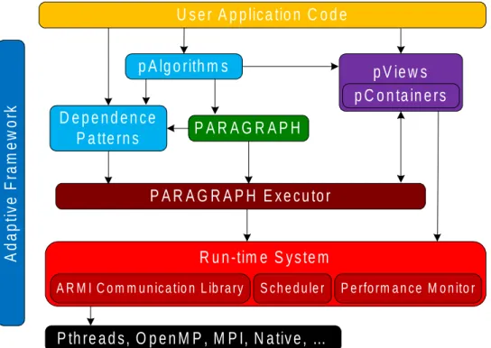
collection of building blocks (as shown in Figure 3.2) for writing parallel programs. These building blocks are commonly referred to as components and include a
collec-(a) (b) free clutter narrow passage blocked (c)
tion of parallel algorithms (pAlgorithms), parallel and distributed data structures
(pContainers) and views to abstract data access in pContainers.
stapl pContainers are similar to the stl containers but much more enriched
and support both static and dynamic parallel and distributed data structures. The
pContainers include pVectors, pArray, pList, pMatrices and pGraphs, which are
parallel versions of vector, array, linked list, matrices and graphs respectively. The
stapl pAlgorithms provide parallel versions of the stl algorithms and are written
in terms of views similar to how stl algorithms are written in terms of iterators.
The stapl P ARAGRAP H abstracts the concept of a task graph needed for par-allel execution. Each task in the task graph consists of a workfunction and a view representing the data on which the workfunction will be applied. stapl also
pro-vides a communication infrastructure called an adaptive runtime system (ARM I).
ARM I is built on MPI and hides machine specific details and provides a uniform communication interface.
Except otherwise noted, all algorithms presented in this work were written in
C+ + and implemented within thestaplframework as staplpAlgorithms. These
pAlgorithms are implemented using the pContainer as data structure. In
partic-ular, we made use of the stapl graph library [83] to represent the parallel data
structures (e.g., the region graph, the roadmap graph, the rapidly-exploring ran-dom tree (RRT)) and a number ofstaplgraph algorithms such as bread-first-search
(BFS), pagerank, connected components, diameter, and single-source shortest path (SSSP).
U s e r A p p lic a tio n C o d e
p A lg o rith m s
p V ie w s
P A R A G R A P H
R u n -tim e S y s te m
P th re a d s , O p e n M P , M P I, N a tiv e , …
A
d
a
p
ti
v
e
F
ra
m
e
w
o
rk
S c h e d u le r P e rfo rm a n c e M o n ito r A R M I C o m m u n ic a tio n L ib ra ryp C o n ta in e rs
D e p e n d e n c e
P a tte rn s
P A R A G R A P H E x e c u to r
4. GRAPH-BASED PARALLEL MOTION PLANNING∗
In this chapter, we discuss our approach for parallelizing graph-based motion planning algorithms. The overall algorithm is shown in Algorithm 4. We discuss the core subroutines of the algorithm in the following sections.
Algorithm 4 Graph-Based Algorithm
Input: An environment env, the number of nodes N, the number of processes p,
the number of regions Nr
Output: A roadmap graph G containingN
1: Let region graph R(V, E) = ∅.
2: Let Rd = SubdivideE into Nr regions.
3: Add a vertex for each region r of Rd to R.
4: for all neighboring regions (r1, r2) Rd) par do
5: Add the edge (r1, r2) to R.
6: end for
7: for all regions vi ∈V par do
8: G← Construct regional roadmap using sequential planner
9: end for
10: for all neighboring regions (vi, vj)∈E par do
11: G← Connect roadmap of regions vi and vj
12: end for
13: return G
4.1 Space Subdivision and Region Graph Construction
In line 2 of Algorithm 4, the environment representing the movable object and the obstacles is subdivided into regions. The subdivision is based on the geometry of the planning space. The planning space may be subdivided into regions using the Cspace
∗Part of the data reported in this chapter is reprinted with permission from “A Scalable Method
for Parallelizing Sampling-Based Motion Planning Algorithms” inProc. IEEE Int. Conf. Robot.
Autom. (ICRA)by S. A. Jacobs, K. Manavi, J. Burgos, J. Denny, S. Thomas, and N. M. Amato,
positional degrees of freedom, i.e., thex,yandz dimensions. A simple illustration of a 2D environment subdivided into nine regions is shown in Figure 4.1(a). We main-tain some user-defined overlap between regions to allow sampling in the portions of the space that are at the boundaries that may facilitate connection between regional roadmaps at a later stage.
The subdivision is represented by aregion graph, whose vertices represent regions and whose edges encode the adjacency information between regions. Figure 4.1(b) shows the region graph corresponding to the subdivision shown in Figure 4.1(a). The algorithm for the region graph construction is shown in Algorithm 5. In addition to geometric and adjacency information, the region graph also maintains additional information that keeps track of the connected components in each region. This additional information is used when connecting adjacent regions.
Algorithm 5 Region Graph Construction
Input: An environment E and the number of regions NR.
Output: A region graphR. LetR =∅.
LetRd = SubDivideSpace(E, NR).
Add a vertex for each region r of Rd toR.
for all neighboring regions (r1, r2) Rd) par do
Add the edge (r1, r2) to R. end for
return R.
4.2 Constructing Regional Roadmaps
Sequel to space subdivision and region graph construction, each processor is as-signed at least one region and the task of building a regional roadmap in its asas-signed region(s) using sequential planner. At this step, any of the existing sampling-based
D E C F I H G B A obsta cle obsta cle A C I G A B E D H F
Figure 4.1: Space subdivision: (a) A 2D environment subdivided into 9 regions, (b) region graph - the 9 vertices represent each of the 9 regions with corresponding color, edges encode the adjacency information between regions.
motion planning algorithms, such as PRM (and its variants) or RRT (and its vari-ants) can be used. This step is independent of the sampling strategy employed. In constructing the regional roadmap, each processor independently generates and connects samples in its assigned region with no communication with other regions. The nodes and edges made at this step are added to the roadmap graph. These nodes and edges represent the valid configurations of the movable object and the connections between the configurations, respectively.To facilitate and streamline the connection at the next step, we keep track of the size and a vertex representative for each connected component (CCIDs) in the regional roadmap. These CCIDs are stored in the region graph for each region.
4.3 Connecting Regional Roadmaps
The final step in constructing the full roadmap is to connect the regional roadmaps. Prior to this step, we track the sizes and number of connected components in each region. The regional graph stores this information which is input to the region con-nection algorithm shown in Algorithm 6. Other inputs to the algorithm include: k, the number of connections to be attempted between adjacent regions, the type of connection method, and a local planner used to verify connections.
For every edge identifying neighboring regions in the region graph, we attempt a connection between candidate node(s) of connected components in the source region to candidate node(s) of connected components in the target region. Even though our implementation is independent of which region connection method is used, for the results presented in this dissertation, we attempt to connect regions based on the size of connected components in each region and the distance between connected com-ponents across regions [84]. For the size-based connection, we attempt connections between a user-defined klargest connected components from the source region andk
Algorithm 6 Region Roadmap Connection
Input: A region graphR, connection method, k number of candidates, local plan-ner lp
Output: A roadmap graph G.
for all edges E R par do
if (connection method == closest) then
sourceCC = select k center of mass based closest CC to target region from
E.source
targetCC = select k center of mass based closest CC to source region from
E.target
end if
if (connection method == largest) then
sourceCC = selectk largest CCs from E.source
targetCC = selectk largest CCs from E.target
end if
for all pairs(sourceCC, targetCC) do
if lp.IsConnectable(sourceCC, targetCC) then
Add the edge(sourceCC, targetCC) to G.
end if end for end for
return G.
largest connected components from the target region. For the distance-based connec-tion, we attempt to connect thek-closest connected components between the regions based on the distance between them. This distance is computed between the centers of mass (a measure of average of all configurations in the connected component) of the two connected components.
4.4 Algorithm Analysis
The original PRM algorithm as reported in [16] requires O(N2) time and O(N) space to construct a roadmap with N configurations. This serves as the basis for our analysis and is used for the complexity of constructing a regional roadmap.
given as: T =Td(Env, nr) + nr X i=1 Tr(i) +Tc(i, j)|ER| (4.1) where T is the sum of the cost of space decomposition Td for a given environment
Env subdivided into nr regions, the cost Tr(i) of roadmap construction in region
ri, for all vi VR, and the cost Tc(i, j) of connecting regional roadmaps in regions
ri and rj, for all (ri, rj) ER. If we make a simplifying assumption that the cost of constructing regional roadmap is the same for all regions vi VR, then equation above can be rewritten as :
T =Td(Env, nr) +Tr(i)|VR|+Tc(i, j)|ER| (4.2) Step 1 involves space decomposition. We assumepprocessors/tasks and that the regions are divided equally among thepprocessors. In this case, space decomposition and region graph construction can be done in O(|VR|+|ER|)/p where VR and ER are the vertices and edges of the region graph, respectively.
Step 2 of Algorithm 3 involves the construction of the regional roadmaps. Since we are assuming there are p regional roadmaps, each of the same size, this implies they will have N/pnodes each, and hence the cost of (sequentially) constructing the PRM roadmap for each region will be O((N/p)2). If regional roadmaps are RRTs
instead, one would use the cost of constructing an RRT of sizeN/phere instead, and similarly for any other desired approach for constructing a regional roadmap.
Inter-processor communication occurs when connecting regional roadmaps. The region graph infrastructure helps to limit both computation and communication to adjacent regions. If we assume a naive connection attempt between every configura-tion in a region to every configuraconfigura-tion in neighboring region, this worst case scenario
will result in O((N/p)2) edge computations plus the cost of communication between
neighboring processors.
Thus, in summary, the time, work and space complexity of this approach can be given as O((N/p)2) time, O((N2)/p) work, andO(N) space respectively.
4.5 Experimental Evaluation
In this section, we analyze the performance of our strategy for parallelizing graph-based motion planning algorithms comparing the results with two similar previous methods. We evaluate the performance of our framework on two different parallel machines for two different motion planning problems. We demonstrate that our approach achieves more scalable performance than the previous parallel algorithms.
4.5.1 Algorithms
We implemented four different algorithms. The first two were based on our pro-posed approach but with two different strategies as the underlying sequential planner. These two implementations are referred to as pSBMP-RRT, a parallel sampling-based motion planning method with RRT as the underlying sequential planner, and pSBMP-PRM, a parallel sampling-based motion planning method with PRM as the underlying sequential planner. For evaluation and comparison, we implemented two additional parallel algorithms: the parallel PRM (pPRM) [21] and parallel sampling-based roadmap of trees (pSRT)[25, 26]. Please note that pPRM and pSRT were im-plemented based on our understanding of how they were described in the literature and it is possible that different implementations may perform better.
4.5.2 Machine Architectures
Our experiment was carried out on two massively parallel computers. The first is a Cray XE6 petascale machine at Lawrence Berkely National Laboratory. It has 6384
nodes and a total of 153,216 cores with 217 TB of memory and peak performance of 1.288 peta-flops. The second machine is a major computing cluster at Texas A&M University. It has a total of 300 nodes, 172 of which are made of two quad core Intel Xeon and AMD Opteron processors running at 2.5GHz with 16 to 32GB per node. The 300 nodes have 2400 cores in all with over 8TB of memory and a peak performance of 24 Tflops.
4.5.3 Motion Planning Problems
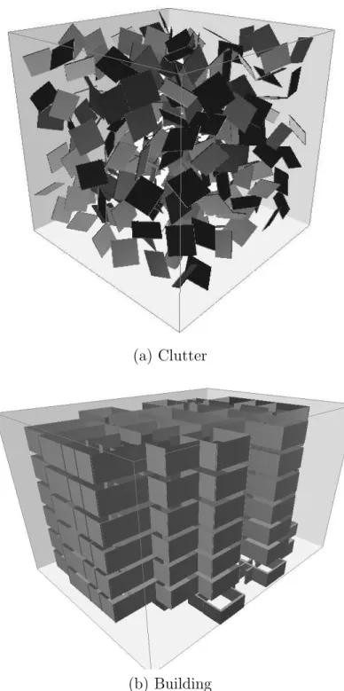
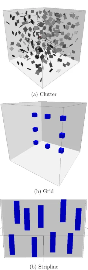
We used two different kinds of environments. The first is a homogeneous cluttered environment with dimensions of 512 x 512 x 512 units. The cluttered elements span thex-axis. The cluttered environment has a total of 216 obstacles, each of size 2 x 64 x 64 units, as shown in Figure 4.2(a). The second environment shown in Figure 4.2(b) is a non-homogeneous cluttered environment. This particular environment models the floor plan of the H.R. Bright building (HRBB), the building that houses the Departments of Computer Science and Engineering and Aerospace Engineering at Texas A&M University.
In both environments, we use two different kinds of robots: a 4 x 4 x 4 unit cube-like rigid body robot and a three-link articulated linkage robot, with each link having dimensions of 7 x 1 x 1 units.
4.5.4 Experimental Results
4.5.4.1 Comparison with Previous Approaches
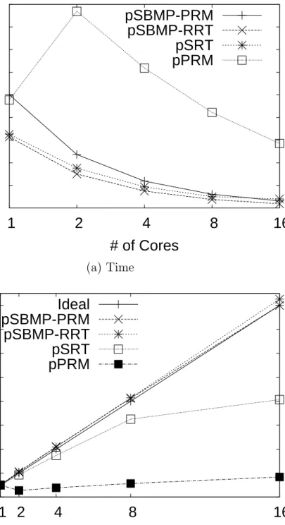
We tested the four algorithms (pSBMP-PRM, pSBMP-RRT, pPRM and pSRT) on the Linux cluster varying the processor count from 1 to 16. The input sample size was fixed at 9600 for each of the four algorithms. Each experiment was run five times and the average maximum time for the 5 runs was computed. Figures 4.3(a) and (b) show the running time and speedup for the four algorithms. From Figure 4.3, one
(a) Clutter
(b) Building
0
100
200
300
400
500
600
700
800
900
1
2
4
8
16
Time(s)
# of Cores
pSBMP-PRM
pSBMP-RRT
pSRT
pPRM
(a) Time0
2
4
6
8
10
12
14
16
1 2
4
8
16
Speedup
# of Cores
Ideal
pSBMP-PRM
pSBMP-RRT
pSRT
pPRM
(b) Speed upFigure 4.3: Comparison of our proposed method (pSBMP-PRM and pSBMP-RRT) to two existing approaches: pPRM and pSRT
will observe that our proposed method (pSBMP-PRM and pSBMP-RRT) achieves good scalability compared to the existing methods. For this particular experiment, we stopped at a processor count of 16 because the two existing algorithms (the pPRM in particular) could no longer scale beyond 16 processor counts. The existing algorithms are limited in scalability primarily because of the inherent interprocessor communication overhead they incurred.
4.5.4.2 Effects of Different Environments and Machine Architectures
We conducted further experiments in order to observe how our method would perform in different environments and machine architectures. Even though these problems exhibit different levels of difficulty and homogeneity leading to differences in running time, we observe that their relative performances are still similar.
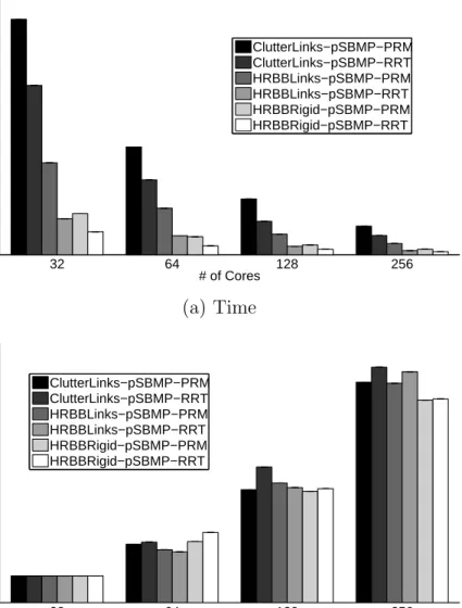
Figure 4.4 shows both the timing and scalability results for three different motion planning problems. The first problem is the cluttered environment with an articu-lated linkage robot (ClutterLinks), the second is the building environment with an articulated linkage robot (HRBBLinks), and the third is the building environment with a rigid body robot (HRBBRigid). We observe that the more difficult the prob-lem, the better the scaling. The basic reason for this is that processors (cores) are fully engaged with computation which in some cases (if the algorithm and exper-iments are properly designed) lowered the overhead cost of idle or inter-processor communication.
We also observe that scalability improves with an increase in sample size. For the same reason as with problem difficulty, increasing sample size ensures that the processors are fully engaged with computation. Figure 4.5 shows results for varying sample size for the articulated linkage robot in a cluttered environment problem. This set of experiments was carried out on the Linux cluster with processor counts
from 32 to 256.
To study scalability and test the limit of our method, we explore further exper-iments on a Cray XE6 petascale machine. In this experiment, we tested processor counts of 240, 480, 720, 960 and 1200. The results are shown in Figure 4.6. We ob-serve that scalability is still possible on a massively parallel machine such as the Cray XE6. The results also suggest that, to the extent possible, our proposed method is independent of machine architecture. Thus, though there may be variance in results, we still expect to see similar performance and scalability across different platforms.
32 64 128 256 0 100 200 300 400 500 600 # of Cores Running Time(s) ClutterLinks−pSBMP−PRM ClutterLinks−pSBMP−RRT HRBBLinks−pSBMP−PRM HRBBLinks−pSBMP−RRT HRBBRigid−pSBMP−PRM HRBBRigid−pSBMP−RRT (a) Time 32 64 128 256 0 1 2 3 4 5 6 7 8 9 # of Cores Scaling(starts at P=32) ClutterLinks−pSBMP−PRM ClutterLinks−pSBMP−RRT HRBBLinks−pSBMP−PRM HRBBLinks−pSBMP−RRT HRBBRigid−pSBMP−PRM HRBBRigid−pSBMP−RRT
(b) Scaling (Processor counts at P= 32, 64, 128, 256)
Figure 4.4: Results from three different motion planning problems on Linux cluster using pSMBP-PRM and pSMBP-RRT methods
0
100
200
300
400
500
32
64
128
256
Time(s)
# of Cores
N=25600
N=153600
N=256000
(a) Time0
1
2
3
4
5
6
7
8
32
64
128
256
Scaling (starts at P=32)
# of Cores
Ideal
N=25600
N=153600
N=256000
(b) Scaling (Processor counts at P= 32, 64, 128, 256)
Figure 4.5: Results from varying input size for the articulated linkage robot in a cluttered environment using pSMBP-PRM method
20
40
60
80
100
120
140
240
480
720
960 1200
Time(s)
# of Cores
pSBMP-PRM
pSBMP-RRT
(a) Time0
1
2
3
4
5
240
480
720
960
1200
Scaling(starts at P=240)
# of Cores
Ideal
pSBMP-PRM
pSBMP-RRT
(b) Scaling (Processor counts at P= 240,480,720,960,1200) Figure 4.6: Higher processor counts on Cray XE6 petascale machine
5. TREE-BASED PARALLEL MOTION PLANNING∗
Inspired by the growth nature of RRT, in this chapter, we discuss a novel parallel and distributed RRT algorithm (Radial RRT). Radial RRTradially subdivides the Cspace into regions, constructs a portion of the tree in each region in parallel, and connects the subtrees, removing cycles if they exist. Unlike the spatial subdivision discussed in Chapter 4, the radial subdivision method discuss in this chapter is well suited for tree-based motion planning algorithm that (radially) grows a tree starting from a single root whereas the previous method builds a tree of multiple roots.
We present a novel radial subdivision for parallelization that is especially suited for RRTs. Starting from the root qroot, we subdivide Cspace into conical regions and build part of the tree (subtrees) in each region. These subtrees are later connected in a manner such that no cycle exists after region connection. We exploit locality by only attempting to connect branches that reside in neighboring regions. Figure 5.1 shows an example for a two dimensionalCspace. Each process builds a branch (shown in different colors) starting at the root that is biased toward their region of Cspace.
5.1 Space Subdivision and Region Graph Construction
Algorithm 7 describes the Cspace subdivision-based RRT computation in detail. Region construction first creates a hypersphere Sd in d-dimensional Cspace centered at qroot ∈Rd with radius r. We generate Nr random points at distance r fromqroot. Each point qi defines a conical region centered around the ray −−−→qrootqi. We construct a region graphG(V, E) where each vertex vi represents a region defined by qi and an
∗Part of the data reported in this chapter is reprinted with the kind permission of IEEE from
“A Scalable Distributed RRT for Motion Planning ” in Proc. IEEE Int. Conf. Robot. Autom.
(ICRA)by S. A. Jacobs, N. Stradford, C. Rodriguez, S. Thomas, and N. M. Amato, 2013. Copyright
Figure 5.1: Example of radial subdivision for a 2D Cspace. Each process concurrently builds a branch (using sequential RRT) rooted at qr and biased toward a target qi (e.g., qn for the black process).
edge (vi, vj) is added if qj is one of the k−closestneighbors of qi. Thus, the edges in the region graph encode the neighborhood information between regions.
5.2 Constructing Regional Subtrees
After region graph construction, we independently (in parallel) run sequential RRT in each region. The RRT construction is done in a way that the tree is biased toward the region target qi. Each region is centered around the random ray −−−−→qroot, qi. Some overlap between regions is allowed so subtrees can explore part of the space in adjacent regions, enabling easier connection between subtrees in the next phase.
5.3 Connecting Regional Subtrees
Using the adjacency information provided by the region graph, we make connec-tion attempts between each region branch and its adjacent neighbors. We check if any edge connection at this point creates a cycle. If a cycle exists, we prune the tree so as to remove any cycles. In the results presented here, tree pruning is performed by running a graph search algorithm. Figure 5.2 shows a simple pictorial illustration
Algorithm 7 Radial Subdivision Distributed RRT
Input: An environmentenv, a rootqroot, the number of nodesN, a stpdfize ∆q, the
number of processes p, the number of regionsNr, a region radius r, the number of adjacent regions k
Output: A tree T containingN nodes rooted at qroot
1: QNr ← generate Nr random points of r distance from qroot 2: Initialize region graph G(V, E) with V ←QNr and E ← ∅
3: for all qi ∈QNr par do
4: neighbors← FindNeighbors(G, qi, k)
5: for all n∈neighbors do
6: G.AddEdge(qi, n)
7: end for
8: end for
9: for all vi ∈V par do
10: T ← ConstructBiasedRRT(env, qroot, N/p,∆q, qi)
11: end for
12: for all (vi, vj)∈E par do
13: ConnectTree(T, vi, vj) 14: if Cycle(T) then 15: Prune(T) 16: end if 17: end for 18: return T
for tree pruning.
5.4 Algorithm Analysis
The complexity analysis of the parallel algorithms for radial subdivision RRT can be broken down into the following phases: the region construction phase, the regional radial RRT construction phase, the region connection phase, and removal of cycles phase. The overall time complexity of the algorithm can be described in terms of these phases as:
Figure 5.2: Tree pruning example, the new edge (purple) between the red and blue branches causes a cycle in the red branch, the dashed edge is identified for removal.
where the total timeT is the sum of the costTd of region graphG(VR, ER) construc-tion for a given environmentEnv subdivided intonr regions with each region having
d neighbors, the cost Tr of constructing sequential Radial RRTs in region ri, for all
vi VR, the cost Tc of connecting neighboring subtrees between adjacent regions ri and rj, for all (ri, rj) ER, and the cost Tcycle of removing cycle that may exist after region connection. In our analysis,prefers to the number of parallel processing elements (processors), we assume there as many regions as number of processors. In other words, nr is some constant factors ofp and nr ≤p. Please note that our anal-ysis assumes a uniform cost of constructing subtrees in each region; this assumption may fail in a situation where the regions are non-uniform.
In the first phase, we construct the region graph ofnrvertices anddnredges. The dominant factor in constructing the region graph is the d-nearest neighbor search, with O(n2