University of New Orleans University of New Orleans
ScholarWorks@UNO
ScholarWorks@UNO
University of New Orleans Theses and
Dissertations Dissertations and Theses
Spring 5-23-2019
StackCBpred: A Stacking based Prediction of
StackCBpred: A Stacking based Prediction of
Protein-Carbohydrate Binding Sites from Sequence
Carbohydrate Binding Sites from Sequence
Suraj GattaniFollow this and additional works at: https://scholarworks.uno.edu/td
Part of the Biological Engineering Commons, Computer Engineering Commons, and the Medicine and Health Sciences Commons
Recommended Citation Recommended Citation
Gattani, Suraj, "StackCBpred: A Stacking based Prediction of Protein-Carbohydrate Binding Sites from Sequence" (2019). University of New Orleans Theses and Dissertations. 2605.
https://scholarworks.uno.edu/td/2605
This Thesis is protected by copyright and/or related rights. It has been brought to you by ScholarWorks@UNO with permission from the rights-holder(s). You are free to use this Thesis in any way that is permitted by the copyright and related rights legislation that applies to your use. For other uses you need to obtain permission from the rights-holder(s) directly, unless additional rights are indicated by a Creative Commons license in the record and/or on the work itself.
This Thesis has been accepted for inclusion in University of New Orleans Theses and Dissertations by an authorized administrator of ScholarWorks@UNO. For more information, please contact [email protected].
StackCBpred: A Stacking based Prediction of Protein-Carbohydrate Binding Sites
from Sequence
A Thesis
Submitted to the Graduate Faculty of the University of New Orleans
in partial fulfillment of the requirements for the degree of
Master of Science in
Computer Science
by Suraj Gattani
B.S. Savitribai Phule Pune University, 2017 May, 2019
ii
Acknowledgement
First of all, I would like to humbly express my profound gratitude to my supervisor Dr. Md. Tamjidul Hoque for being so kind, enduring and at the same time vigilant in every aspect of my research and academic progress during the whole time I have been here at University of New Orleans. He has helped me with the valuable suggestions and commendable support throughout the way towards completion of my thesis.
Secondly, I would like thank Dr. Christopher M. Summa and Dr. Shaikh M. Arifuzzaman for their kind consent to be a board member of my thesis committee, despite their hectic schedule and important other priorities.
I must mention my lab partner and friend Avdesh Mishra. He has been tireless to explain every nuance again and again till I understand any concept. I must appreciate his continuous guidance, critical and insightful advice, helpful and inspiring criticism to contribute equally in this work. I would also like to thank my family and friends for their immense support.
I would also like to thank University of New Orleans for providing me an excellent environment for research.
iii
Table of Contents
List of Tables ... iv List of Figures ... vi ABSTRACT ... vii Chapter 1 Introduction... 1Chapter 2 Literature Review ... 3
2.1 Background and Related Works ... 3
2.2 Review of Machine Learning Methods... 7
2.2.1 Support Vector Machine (SVM) ... 7
2.2.2 Logistic Regression (LogReg) ... 8
2.2.3 Extra Tree Classifier (ETC) ... 9
2.2.4 Random Decision Forest (RDF) ... 10
2.2.5 K Nearest Neighbors (KNN) ... 10
2.2.6 Bagging Classifier ... 11
2.2.7 Gradient Boosting Classifier (GBC)... 12
2.2.8 XGBoost (XGB)... 12
Chapter 3 Experimental Materials ... 14
3.1 Datasets ... 14
iv
3.1.2 Test Datasets ... 15
3.2 Features Extraction ... 16
3.2.1 Position Specific Scoring Matrix (PSSM) and Monogram (MG) ... 16
3.2.2 Accessible Surface Area (ASA) and Secondary Structure (SS) ... 17
3.2.3 Half Sphere Exposure (HSE) and Torsion angles ... 17
3.2.4 Physiochemical Properties ... 17
3.2.5 Molecular Recognition Features (MoRFs) ... 18
Chapter 4 Methodology ... 19
4.1 Feature Selection ... 19
4.2 Performance Evaluation ... 19
4.3 Parameter Optimization and Window Selection ... 21
Chapter 5 Stacking ... 24
5.1 Performance Comparison on Benchmark Dataset ... 30
5.2 Performance Comparison using Independent Test Datasets ... 32
5.3 Statistical Significance Test ... 34
Chapter 6 Conclusions ... 37
References ... 39
v
List of Tables
Table 1: Name and definition of the evaluation metric. ... 20 Table 2: Comparisons of various machine learning algorithms on the benchmark dataset using
10-fold CV. ... 26 Table 3: Pair-wise correlation analysis of the probability distribution given by the
base-classifiers on TS49. ... 29 Table 4: Comparisons of stacked models with a different set of base classifiers on benchmark
dataset through 10-fold CV. ... 31 Table 5: Comparisons of StackCBPred with SPRINT-CBH on the benchmark dataset. ... 32 Table 6: Comparisons of StackCBPred with SPRINT-CBH on balanced and imbalanced
independent test dataset, TS49. ... 33 Table 7: Comparisons of StackCBPred with SPRINT-CBH on imbalanced independent test
dataset, TS88. ... 34 Table 8: Here, the contingency table is formed by comparing the predicted results of
StackCBPred and SPRINT-CBH with actual class labels. ... 36 Table 9: Here, the contingency table is formed by comparing the predicted results of
vi
List of Figures
Figure 1: A simple two class classification problem is shown here. The squares and circles shaped data points belong to two different classes. The classes may be separated by many different decision boundaries as shown on the left side. But the optimal hyperplane shown on the right side has the maximum margin and it is considered as the decision boundary. . 8 Figure 2: The decision function used to obtain the probability for particular class. ... 9 Figure 3: The initial data, calculation of distance and finding neighbors and voting for labels ... 11 Figure 4: Performance comparison of SVM based models created from different sliding window
sizes. The sensitivity, specificity and balanced accuracy are reported. The optimal size of the window and the corresponding performance scores are marked by a black rectangle.23 Figure 5: Illustration of the framework of the final predictor, StackCBPred, which is principally
the Model-1 with another version of SVM in the meta layer. ... 27 Figure 6: Comparison of ROC and AUC scores given by StackCBPred and SPRINT-CBH on
vii
ABSTRACT
Carbohydrate-binding proteins play vital roles in many vital biological processes and study of these interactions, at the residue level, are useful in treating many critical diseases. Analyzing the local sequential environments of the binding and non-binding regions to predict the protein-carbohydrate binding sites is one of the challenging problems in molecular and computational biology. Prediction of such binding sites, directly from sequences, using computational methods, can be useful to quickly annotate the binding sites and guide the experimental process. Because the number of carbohydrate-binding residues is significantly lower than carbohydrate-binding residues, most of the methods developed are biased towards over-predicting the non-carbohydrate-binding residues. Here, we propose a balanced predictor, called StackCBPred, which utilizes features, extracted from an evolution-driven sequence profile, called the position-specific scoring matrix (PSSM) and several predicted structural properties of amino acids to effectively train a stacking-based machine learning method for the accurate prediction of protein-carbohydrate binding sites.
1
Chapter 1
Introduction
Protein-Carbohydrate interactions are crucial in many biological processes with implications to drug targeting and gene expression. The nature of protein-carbohydrate interactions may be studied at an individual residue level by analyzing local sequence and structure environments in binding regions in comparison to non-binding regions, which provides an inherent control for such analyses. Very few methods have been explored to predict the carbohydrate binding sites such as docking, structure-based, etc. Experimental methods require structures, but it is very difficult to find structures for all the proteins which increases the experimental cost. The existing methods lack the ability to effectively predict binding sites and thus, it is essential to identify new features and effective machine learning techniques that can help in improved binding site predictions.
In the modern scientific world bioinformatics has attained a very crucial position as a research discipline, promising the potential of benefitting human endeavor to understand and analyze biological phenomenon. In this study, we have predicted the protein-carbohydrate binding sites through sequence of amino acids. The fasta sequences for the proteins have been obtained from the PDB database. To further enhance the overall input sequence, the redundant protein sequences which are identical and small in length have been removed. We divided this data in train and test sets including 100 and 49 sequences respectively. We also collected another test set to examine the robustness of the predictor. After data collection, we collected various features extracted from the sequential and structural properties of proteins.
2
We collected various features such as Position Specific Scoring Matrix (PSSM), Monogram (MG), Accessible Surface Area (ASA), Secondary Structure (SS), Half Sphere Exposure (HSE), Torsion Angles, Physiochemical Properties and Molecular Recognition Features (MoRFs). We performed feature selection and windowing method to improve the performance of predictor. We implemented the Stacking method to build the StackCBPred predictor for carbohydrate-binding sites prediction. We employed several state-of-the-art learning methods in the base-classifiers to supply the meta base-classifiers important information and obtain better performance for predictions. The eight different machine learning algorithms we examined are (a) Support Vector Machines (SVM), (b) Gradient Boosting Classifier (GBC), (c) Bagging Classifier (BAG), (d) Extra Tree Classifier (ETC), (e) Random Decision Forest (RDF), (f) K-Nearest Neighbor (KNN) (g) Logistic Regression (LOGREG), and (h) XGBoost (XGB). We calculated the pearson correlation coefficient of the machine learning algorithms created different models. In the base classifier, we used SVM, LOGREG, KNN and ETC whereas in the meta classifier we employed SVM.
The remainder of this paper proceeds as follows. We review the evolution of the relevant theories and underpinning theoretical aspect of our proposed approaches in Chapter 2. Chapter 3 discusses our approach for data and feature collections. The approach for feature selection, performance evaluation, window selection and parameter optimization is discussed in Chapter 4. Chapter 5 elaborates the stacking method and performance comparison to other machine learning methods. Finally, Chapter 6 concludes the proposed protein-carbohydrate binding sites predictor.
3
Chapter 2
Literature Review
2.1 Background and Related Works
Organisms need four types of molecules: nucleic acids, proteins, carbohydrates (or polysaccharides) and lipids for life, which are usually referred to as the molecules of life [1]. Carbohydrates are often considered as the third important molecule of life, after DNA and proteins. Carbohydrates interacts with many different protein families which include lectins, antibodies, sugar transporters and enzymes [2]. Protein-carbohydrate interactions are responsible for various biological processes, including intercellular signaling, cellular adhesion, cellular recognition, protein folding, subcellular localization, ligand recognition and developmental process [3-5]. In fact, carbohydrates of one or the other type generally cover the surface of living cells in all organisms [6]. These carbohydrates play important roles in the defense for human cell against pathogens [7]. Moreover, some pathogens such as influenza use these carbohydrates on the outside of the human cell to gain entry [8]. The proteins, which recognize and bind to the cell-surface carbohydrates, are useful as biomarkers or drug targets [8-11]. The study of protein-carbohydrate interactions is usually carried out by experimental techniques including X-ray crystallography, nuclear magnetic resonance (NMR) spectroscopy study, molecular modeling, fluorescence spectrometry, and dual polarization interferometry. However, protein-carbohydrate interactions are challenging to study experimentally because of the weak binding affinity and synthetic complexity of individual carbohydrates [6]. Therefore, the prediction of protein-carbohydrate interactions through a computational approach becomes
4
essential. This motivated us to develop an effective computational predictor for effective identification and characterization of protein-carbohydrate binding sites.
Study of protein-carbohydrate interactions using computational methods mainly focuses on locating the sites of proteins that bind to carbohydrates. One of the promising computational techniques is docking. Docking methods are often used to predict the orientation of the carbohydrate in the binding site [2]. Docking algorithms such as Autodock [12], GLIDE [13], Dock [14], etc. consider the orientation of the dangling groups, such as, hydroxyl groups and hydrogen bond network that stabilizes the complex, and the conformational behavior of the glycosidic bonds for oligosaccharides [2]. On the other hand, Taroni et al. [15] proposed the first bioinformatics approach for predicting protein-carbohydrate binding sites from a known protein structure. In their work, six parameters of amino acids were evaluated, which includes solvation potential, residue propensity, hydrophobicity, planarity, protrusion, and relative accessible surface area. A simple combination of three of the parameters (residue propensity, protrusion and relative accessible surface area) out of six were found to distinguish the observed binding sites with an overall accuracy of 65% for a set of 40 protein-carbohydrate complexes. Likewise, Sujatha and Balaji developed a method called COTRAN for predicting protein-galactose binding sites [16]. They utilized the combination of geometrical and structural characteristics such as solvent accessibility and secondary structure type that allowed proper detection of potential galactose-binding sites. Kulharia et al. developed a program called InCa-SiteFinder for predicting non-covalent inositol and carbohydrate binding sites on the surface of the protein structure [17]. They employed van der Waals interaction energy between protein and a probe and amino acid propensities as the parameters to locate and predict carbohydrate-binding sites. A continuous
5
surface pocket interacting with protein-probes was considered a binding site. Nassif et al. proposed a glucose-binding site classifier which considers the sugar-binding pocket as a spherical spatio-chemical environment and represents it as a vector of geometric and chemical features which includes charges, hydrophobicity, hydrogen bonding and more [18]. They employed random decision forest for feature selection and used selected geometric and chemical features to train support vector machines (SVM) for predicting protein-glucose binding sites. Tsai et al. predicted binding sites by employing three-dimensional probability density distribution of interacting atoms in protein surfaces as input to the neural networks and SVM [19]. In the recent past, an energy-based approach for the identification and analysis of binding site residues in protein-carbohydrate complexes has been proposed [20]. Through this study, it was found that 3.3% of residues are identified as binding sites in protein-carbohydrate complexes whereas the binding site residues in protein-protein, protein-RNA, and protein-DNA complexes are 10.8%, 7.6%, and 8.7% respectively. Furthermore, the binding propensity analysis performed in this study indicates the propensity the amino acid of Tryptophan (TRP) to interact with the carbohydrates through aromatic-aromatic interactions. More recently, Shanmugam et al.
proposed a method to identify and analyze the residues, which are involved in both the folding and binding of protein-carbohydrate complexes [21]. Stabilizing residues were identified by using knowledge of hydrophobicity, long-range interactions, and conservations, as well as binding site residues, were identified using a distance cutoff of 3.5Å between heavy atoms in protein and ligand. Residues which were common in stabilizing and binding were termed as key residues. Some of the interesting findings of the work indicate that most of the key residues are present in
6
The structure-based methods discussed above, rely on protein structures that are often not available, which makes the sequence-based method invaluable. The first sequence-based method for protein-carbohydrate binding sites prediction was developed by Malik and Ahmad in 2007 [8]. In their work, Malik and Ahmad used only the evolutionary attributes called PSSM as input to the neural network to create a predictive model. Their method achieved the average of 87% sensitivity and 23% specificity while tested by leave-one-out technique on a dataset of 40 protein-carbohydrate complexes. After a year less than a decade, Taherzadeh et al. proposed a method, called SPRINT-CBH, which used PSSM profiles with additional information on sequence and predicted solvent accessible surface area as features to develop an SVM based predictor in 2016 [6]. As reported, SPRINT-CBH achieved the average of 18.8% sensitivity and 99.6% specificity while tested using 10-fold cross-validation (CV) on a dataset of 102 protein-carbohydrate complexes and 22.3% sensitivity and 98.8% specificity while tested using independent test set of 50 protein-carbohydrate complexes. Both aforementioned methods suffer from the problem of imbalanced prediction accuracies. These methods either yield a high sensitivity and low specificity or vice versa. Thus, the existing methods are limited in their ability to effectively predict binding sites and explain how protein-carbohydrate interaction occurs. Therefore, it becomes essential to identify new features and effective machine learning techniques that can help in improved binding site prediction as well as help interpret protein-carbohydrate interactions.
While there are still very few methods for predicting protein-carbohydrate binding sites, many other methods have been established for binding site and binding proteins prediction in the area of protein-protein [22-25], protein-peptide [26-29], protein-DNA [30-33], protein-RNA
7
[34-37] and protein-ligand [38-41] interactions. Several of the aforementioned sequence-based methods have shown that the use of evolution-derived and predicted sequence and structure-based features can significantly improve the overall performance of binding site prediction.
2.2 Review of Machine Learning Methods
In this study, we investigated different descriptors, which include information extracted from the evolutionary profile as well as predicted sequence and structural properties. Useful feature groups were selected by feature selection to build a stacking-based classifier called StackCBPred. We examined the following machine learning methods to develop this predictor.
2.2.1 Support Vector Machine (SVM)
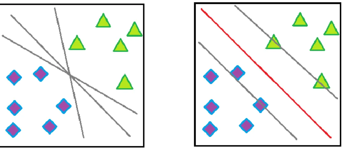
A Support Vector Machine (SVM) [42] is a discriminative classifier formally defined by a separating hyperplane. In this algorithm, each data item is plotted as a point in n-dimensional space (where n is number of features) with the value of each feature being the value of a particular coordinate. To separate the two classes of data points, there are many possible hyperplanes that could be chosen. But the objective is to find a plane that has the maximum margin, i.e. the maximum distance between data points of both classes shown in Figure 1. Maximizing the margin distance provides some reinforcement so that future data points can be classified with more confidence.
8
Figure 1: A simple two class classification problem is shown here. The squares and circles shaped data points belong to two different classes. The classes may be separated by many different decision boundaries as shown on the left side. But the optimal hyperplane (in red) shown on the right side has the maximum margin and it is considered as the decision boundary.
2.2.2 Logistic Regression (LogReg)
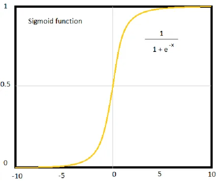
Logistic regression [43] is a technique for analyzing problems in which there are one or more independent variables that determine a dependent variable (outcome). In most cases, the dependent variable is a dichotomous variable (in which there are only two possible outcomes). The goal of logistic regression is to find the best fitting model to describe the relationship between the dichotomous characteristic of interest (dependent variable) and a set of independent (predictor or explanatory) variables. It transforms its output using the logistic sigmoid function in Figure 2. to return a probability value which can be mapped to the discrete classes. To avoid overfitting, regularization techniques are used (which is any modification we make to a learning algorithm that is intended to reduce the generalization error).
9
Figure 2: The decision function used to obtain the probability for particular class.
2.2.3 Extra Tree Classifier (ETC)
The Extra-Tree method [44] (standing for extremely randomized trees) was proposed with the main objective of further randomizing tree building in the context of numerical input features, where the choice of the optimal cut-point is responsible for a large proportion of the variance of the induced tree. The method drops the idea of using bootstrap copies of the learning sample and it selects a cut-point at random. From a statistical point of view, dropping the bootstrapping idea leads to an advantage in terms of bias, whereas the cut-point randomization has often an excellent variance reduction effect. This method has yielded state-of-the-art results in several high-dimensional complex problems.
10 2.2.4 Random Decision Forest (RDF)
Random Decision Forests [45] are an ensemble learning method for classification, regression and other tasks. RDF operate by constructing a multitude of decision trees at training time and outputting the class that is the mode of the classes (classification) or mean prediction (regression) of the individual trees. Random decision forests correct for decision tree’s habit of overfitting to their training set. Random Forest adds additional randomness to the model, while growing the trees. Instead of searching for the most important feature while splitting a node, it searches for the best feature among a random subset of features. This results in a wide diversity that generally results in a better model.
2.2.5 K Nearest Neighbors (KNN)
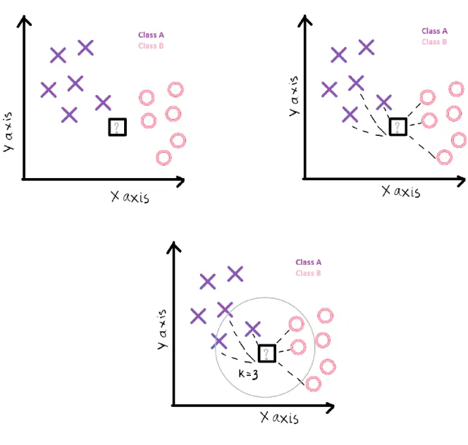
K nearest neighbors [46] is a simple algorithm that stores all available cases and classifies new cases based on a similarity measure. KNN has been used in statistical estimation and pattern recognition as a non-parametric technique. A case is classified by a majority vote of its neighbors, with the case being assigned to the class most common amongst its K nearest neighbors measured by a distance function. If K = 3, then the case is simply assigned to the class of its 3 nearest neighbors shown in Figure 3.
11
Figure 3: The initial data, calculation of distance and finding neighbors and voting for labels
2.2.6 Bagging Classifier
Bagging [47] is a “bootstrap” ensemble method that creates individuals for its ensemble by
training each classifier on a random redistribution of the training set. Each classifier's training set is generated by randomly drawing, with replacement, N examples - where N is the size of the original training set; many of the original examples may be repeated in the resulting training set
12
while others may be left out. Each individual classifier in the ensemble is generated with a different random sampling of the training set and subsequently aggregates their individual predictions to yield a final prediction. It is useful for reducing variance in the prediction.
2.2.7 Gradient Boosting Classifier (GBC)
GBC [48] builds an additive model in a forward stage-wise fashion; it allows for the optimization of arbitrary differentiable loss functions. GBC involves three elements: (a) a loss function to be optimized, (b) a weak learner to make predictions and (c) an additive model to add weak learners to minimize the loss function. The objective of GBC is to minimize the loss of the model by adding weak learners in a stage-wise fashion using a procedure similar to gradient descent. The existing weak learners in the model are remained unchanged while adding a new weak learner. The output from the new learner is added to the output of the existing sequence of learners in an effort to correct or improve the final output of the model
2.2.8 XGBoost (XGB)
The implementation of XGB [49] offers several advanced features for model tuning, computing environments and algorithm enhancement. It is capable of performing the three main forms of gradient boosting (Gradient Boosting (GB), Stochastic GB and Regularized GB) and it is robust enough to support fine tuning and addition of regularization parameters. However, XGB uses a more regularized model formalization to control over-fitting, which results in better performance. In addition to the better performance, XGB is designed to provide higher computational speed.
13
By exploring the aforementioned machine learning methods, we developed sequence-based unbiased and balanced predictor of non-covalent protein-carbohydrate binding sites. The StackCBPred was trained and cross-validated by 100 carbohydrate-binding proteins and independently tested by two different test sets containing 50 and 88 proteins with known high-resolution protein-carbohydrate complex structures, respectively. As the dataset contain significantly more non-binding residues than binding residues, StackCBPred was trained with a balanced dataset obtained by employing the undersampling technique with an aim to design a more balanced predictor. The development of StackCBPred offered a significant improvement in sensitivity and balanced accuracy based on the benchmark and independent test data when compared to the existing sequence-based binding predictor. We believe that the superior performance of StackCBPred will motivate the researchers to use this method to identify protein-carbohydrate binding sites directly from sequence and utilize the outcomes for drug targeting. In addition, the stacking-based machine learning technique and features proposed in this work could be applied to solve various other biologically important problems.
14
Chapter 3
Experimental Materials
In this section, we describe the approach taken to prepare data sets, aggregation of input features and performance evaluation.
3.1
Datasets
In this study, our focus is to capture the residue-patterns of different protein-carbohydrate binding sites from the protein sequence alone. We have used three different datasets to train and test the performance of the predictor.
3.1.1 Benchmark Dataset
We collected the benchmark dataset [6] that contains a total of 102 high-resolution carbohydrate-binding protein sequences. However, in our implementation, we only used 100 high-resolution carbohydrate-binding protein sequences for training and cross-validation as two of the sequences contain non-standard amino acid and the physicochemical properties of the non-standard amino acids could not be obtained. From the benchmark dataset of 100 sequences, we obtained a total of 26,986 residues, of which, 1028 residues are binding, and the rest are non-binding. To avoid bias caused by a large number of non-binding residues, a balanced dataset was prepared following an undersampling approach [50] by randomly selecting a number of non-binding residues equal to the number of non-binding residues. This resulted in a benchmark dataset, which consists of 1028 binding and an equal number of non-binding residues.
15 3.1.2 Test Datasets
Furthermore, we collected an independent test dataset [6] to compare the performance of StackCBPred with each predictor. This dataset consists of 50 high-resolution carbohydrate-binding protein sequences, of which 49 were used in our implementation, discarding one for having the nonstandard amino acids in the sequence information. Here and after we represent this test dataset as TS49. From TS49 sequences, we obtained a total of 13,738 residues of which 508 residues are binding and the rest are non-binding. Using similar undersampling approach as above, a balanced independent test set was prepared which consist of 508 binding and an equal number of non-binding residues.
To further test the performance of our predictor, we collected an additional dataset PROCARB604 from PROCARB [51] database. The proteins whose ID’s matched to the protein ID’s
that were present in either the benchmark or the independent test dataset mentioned above, were removed from this new dataset. Next, the redundant proteins with a sequence identity
cutoff of ≥ 30% according to BLAST-CLUST [52] were removed. Finally, the dataset, which consists of 88 protein-carbohydrate complexes was obtained. Here and after we represent this dataset as TS88. This new TS88 dataset consists of 688 binding residues. Using an undersampling approach, we prepared a balanced dataset which contains 688 binding and an equal number of non-binding residues.
16
3.2
Features Extraction
We collected various useful features which include information extracted from evolutionary profiles as well as predicted sequential and structural properties of proteins, which we describe in this section.
3.2.1 Position Specific Scoring Matrix (PSSM) and Monogram (MG)
PSSM captures the evolution derived information in proteins. Evolutionary information is very impactful for protein function annotation in biological analysis and is widely used in many studies [26, 33, 53-57]. Furthermore, evolutionarily conserved residues are found to play crucial functional roles such as binding [58]. For this study, we obtained the normalized PSSM values for every residue in protein sequence from DisPredict2 [55] program. DisPredict2 internally executes three iterations of PSI-BLAST [59] against NCBI’s non-redundant database to generate a PSSM profile and subsequently converts it to normalized PSSM by dividing each value by a value of 9. PSSM is a matrix of L×20 dimensions, where L is the length of the protein. The rows in PSSM represent the position of amino acid in the sequence and the columns represent the 20 standard amino acid types. Hence, every residue in the protein sequence is encoded by a 20-dimensional feature vector. In addition, the PSSM score was further extended to compute monogram feature [60], which is obtained by taking the sum of the scores over the length of the protein for 20 standard amino acid types. This resulted in 1 feature for every amino acid.
17
3.2.2 Accessible Surface Area (ASA) and Secondary Structure (SS)
ASA and SS are predicted structural features that are found to be highly effective for binding site prediction. We used the DisPredict2 program to obtain predicted ASA and SS probabilities for helix, coil, and beta-sheet at the residue level. DisPredict2 internally uses a program called SPINE-X [61] to predict ASA and SS probabilities directly from the protein sequence.
3.2.3 Half Sphere Exposure (HSE) and Torsion angles
HSE is a measure of protein solvent exposure that was first introduced in [62]. HSE measures how buried amino acid residues are in protein conformation. The calculation of HSE is obtained by dividing a contact number (CN) sphere into two halves by the plane perpendicular to the Cβ-Cα
vector. This simple division of the CN sphere produces two different measures, called HSE-up and HSE-down. In this study, we used these two measures as features which were extracted from the SPIDER3 program [63-65]. Additionally, protein backbone structure can be described by torsion
angles Phi (φ) and Psi (ψ). This local structure descriptor is important for understanding and
predicting protein structure, function, and interactions. In our study, we employed predicted φ and ψ angles as features which were also extracted from SPIDER3 program.
3.2.4 Physiochemical Properties
Seven representative physiochemical attributes of the amino acids, which include steric parameters, hydrophobicity, volume, polarizability, isoelectric point, helix probability, and sheet probability [66] were collected, and fed as features to capture the chemical description of the
18
residues that can transiently interact with carbohydrates. As these features are inherently encoded within DisPredict2, we directly extracted these features from the DisPredict2 [55].
3.2.5 Molecular Recognition Features (MoRFs)
Post-translational modifications (PTMs) can induce disorder-to-order transitions of intrinsically disordered proteins (IDPs). IDPs can transition from disorder to order due to binding to other proteins, nucleic acids, lipids, carbohydrates and other small molecules [67, 68]. MoRFs are key to the biological function of IDPs located within long disordered protein sequences [69]. Thus, to inherently capture functional properties of IDPs which may bind to carbohydrates, we employed a single predicted MoRFs score as a feature in this work. We obtain the MoRFs feature from OPAL [69].
19
Chapter 4
Methodology
4.1 Feature Selection
To identify the features that support the performance of the classifier, we applied a simple incremental feature selection (IFS) approach. IFS begin with the empty feature set and a feature group is added to the feature set if the addition of the feature group improves the performance of the predictor. In case, the accuracy of the predictor is reduced by adding the new feature group, this feature group is discarded, and a new feature group is tested in an iterative fashion. For IFS we used the benchmark dataset to train and TS49 dataset to test the GBC predictor. We initially collected thirty-nine features, of which, we discarded six features based on IFS. The three secondary structure features and three MoRFs features were removed as these features did not help improve the performance of the predictor.
4.2 Performance Evaluation
Performance of the StackCBPred was evaluated by 10-fold CV as well as using the independent test. In 10-fold CV, the dataset is segmented into 10 parts, which are each of about equal size. When a fold is set aside for testing, the other 9 folds are used to train the classifier. This process is repeated until each fold has been set aside once for testing and then the test accuracies of each fold are combined to find the average [70]. On the other hand, to perform the independent test, the classifier is trained with the validation dataset and then tested using the independent test dataset.
20
Table 1: Name and definition of the evaluation metric.
Name of Metric Definition
True Positive (TP) Correctly predicted carbohydrate-binding residues True Negative (TN) Correctly predicted non-carbohydrate-binding residues False Positive (FP) Incorrectly predicted carbohydrate-binding residues False Negative (FN) Incorrectly predicted non-carbohydrate-binding
residues Recall/Sensitivity (Sens.) /True Positive Rate
(TPR)
𝑇𝑃 𝑇𝑃 + 𝐹𝑁
Specificity (Spec.) /True Negative Rate (TNR) 𝑇𝑁
𝑇𝑁 + 𝐹𝑃
Fall Out Rate (FOR) /False Positive Rate (FPR)
𝐹𝑃 𝐹𝑃 + 𝑇𝑁
Miss Rate (MR) /False Negative Rate (FNR) 𝐹𝑁
𝐹𝑁 + 𝑇𝑃
Accuracy (ACC) 𝑇𝑃 + 𝑇𝑁
𝐹𝑃 + 𝑇𝑃 + 𝑇𝑁 + 𝐹𝑁
Balanced Accuracy (BACC)
1
2 (𝑇𝑃 + 𝐹𝑁𝑇𝑃 +𝑇𝑁 + 𝐹𝑃𝑇𝑁 )
Precision (Prec.) 𝑇𝑃
𝑇𝑃 + 𝐹𝑃
F1 score (Harmonic mean of precision and recall)
2𝑇𝑃 2𝑇𝑃 + 𝐹𝑃 + 𝐹𝑁
Mathews Correlation Coefficient (MCC) (𝑇𝑃 ∗ 𝑇𝑁) − (𝐹𝑃 ∗ 𝐹𝑁)
√(𝑇𝑃 + 𝐹𝑁) ∗ (𝑇𝑃 + 𝐹𝑃) ∗ (𝑇𝑁 + 𝐹𝑃) ∗ (𝑇𝑁 + 𝐹𝑁)
We used various performance evaluation metrics listed in the Table 1. to test the accuracy of our proposed method as well as to compare it with the existing method. In addition, we used AUC and ROC performance evaluation metrics. AUC is the area under the receiver operating characteristics (ROC) curve and is used to evaluate a predictor to see how well it separates two classes of information, which is, in this case, carbohydrate binding and non-binding residues.
21
4.3 Parameter Optimization and Window Selection
In this section, we describe the optimized parameters and window size used for the machine learning algorithms to improve the performance of the predictor. We tried several algorithms with different principles as the results of the classifiers may vary with the type of data and they are described below:
i) SVM: We employed SVM [42] with the radial basis function (RBF) kernel as one of the classifiers to be used in stacking framework. The performance of SVM with the RBF kernel relies on two parameters C, and γ. The RBF kernel parameter γ and the cost parameter C are optimized to achieve the best 10-fold CV balanced accuracy using a grid search [71] technique. The optimal values of the parameters of the SVM were found to be C = 21.24and γ = 2-8.75.
ii) LOGREG: We implemented LOGREG [43, 70] with L2 regularization as another classifier to be used in staking framework. The parameter, C which controls the regularization strength is optimized to achieve the best 10-fold CV balanced accuracy using grid search [71]. In our implementation, the optimal value of the parameter, C was found to be 2.3784.
iii) ETC: We employed extremely randomized tree or ETC [44] as another classifier to be used in stacking framework. We constructed the ETC model with 1,000 trees and the quality of a split was assessed by the Gini impurity index.
iv) RDF: RDF [45] creates a set of decision trees from randomly selected subset of training set. It then aggregates the votes from different decision trees to decide the final class of the test object. In our implementation of the RDF, we used bootstrap samples to construct 1,000 trees in the forest.
22
v) KNN: KNN [46] operates by learning from the K number of training samples closest in distance to the target point in the feature space. In this work, the value of K was set to 9 and all the neighbors were weighted uniformly.
vi) BAG: BAG [47] method aggregates their individual predictions to yield a final prediction. In our study, BAG classifier was fit on multiple subsets of data with the repetitions using 1,000 decision trees, and the outputs were combined by weighted averaging.
vii) GBC: GBC [48] builds an additive model in a forward stage-wise fashion; it allows for the optimization of arbitrary differentiable loss functions.Here, we used 1,000 bosting stages where a regression tree was fit on the negative gradient of the deviance loss function. The learning rate and the maximum depth of each regression tree were set to 0.1 and 3, respectively.
viii) XGB: As GBC, XGB [49] also follows the principle of gradient boosting. In our implementation of the XGB, we used 100 bosting stages with a soft prob learning objective, where the number of classes was set to 2 as we are dealing with a binary classification problem of carbohydrate-binding and non-carbohydrate-carbohydrate-binding residues. The values of the additional parameters: learning rate, maximum depth, minimum child weight, and subsample ratio were set to 0.1, 3, 5 and 0.9, respectively.
23 Window Selection
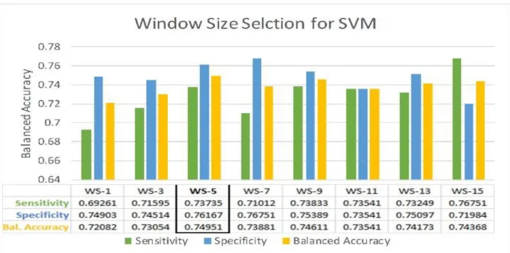
An optimal size of the sliding window (W) was searched to determine the number of residues around a target residue, which can moderate the interaction between protein and carbohydrate. We designed 8 different models of every machine learning classifier with 8 different window sizes (1, 3, 5, 7, 9, 11, 13 and 15). Window size for which the classifier yields the highest 10-fold CV balanced accuracy on benchmark dataset was selected as the optimal window size for that classifier.
We found that the optimal window size for different classifiers varies. For example, the optimal window size for the SVM was found to be 5 (see Figure 4) whereas, for the KNN it was 1. In this study, the optimal window size for every classifier was separately identified to design an accurate and effective predictor.
Figure 4: Performance comparison of SVM based models created from different sliding window sizes. The sensitivity, specificity and balanced accuracy are reported. The optimal size of the window and the corresponding performance scores are marked by a black rectangle.
24
Chapter 5
Stacking
The idea of a stacking based machine learning technique [72] which has recently been successfully applied to solve some interesting bioinformatics problems [26, 33, 73-75] is utilized in this work to develop the StackCBPred predictor for carbohydrate-binding sites prediction. Stacking is an ensemble approach, which obtains the information from multiple models and aggregates them to form a new model. In stacking, the information gained from more than one predictive models minimize the generalization error rate and yields more accurate results.
A stacking framework includes two-stages of learners. The classifiers of the first-stage are called base-classifiers. More than one base-classifier employed in the first-stage. Likewise, the classifiers of the second-stage are called meta-classifiers. Using meta-classifier, the prediction probabilities from the base-classifiers are combined to reduce the generalization error. To supply the meta-classifier with significant information on the problem space, the classifiers that are different from one another based on their underlying operating principles are used as the base-classifiers.
To find the base-classifiers and meta-classifiers to use in the first and second-stage of stacking framework, we examined eight different machine learning algorithms: (a) Support Vector Machines (SVM) [42], (b) Gradient Boosting Classifier (GBC) [48], (c) Bagging Classifier (BAG) [47], (d) Extra Tree Classifier (ETC) [44], (e) Random Decision Forest (RDF) [45], (f) K-Nearest Neighbor (KNN) [46] , (g) Logistic Regression (LOGREG) [43, 70] and (h) XGBoost (XGB) [49].
25
algorithms to be used as the base-classifiers for the stacked model, we evaluate four different combinations of base-classifier which are:
1. Model-1: includes SVM, LOGREG, KNN, and ETC.
2. Model-2: includes SVM, LOGREG, KNN, and RDF.
3. Model-3: includes SVM, LOGREG, KNN, and BAG.
4. Model-4: includes GBC, LOGREG, and KNN.
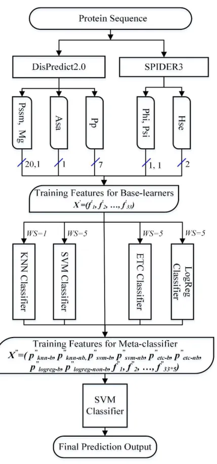
Model-1, Model-2, and Model-3 are constructed to include classifiers that are different from each other based on the underlying principles of learning. Here, the tree-based classifiers ETC, RDF and BAG are individually combined with the other three classifiers, SVM, LOGREG and KNN to learn different information from the problem-space. On the other hand, Model-4 is formed by the pair-wise correlation analysis of the residue-wise probabilities given by the individual classifiers. Three of the classifiers, with the least Pearson correlation coefficient, are selected as base-classifiers. For all the above combinations, SVM is used as a meta-classifier. The 10-fold CVs of the above four combinations indicate that the Model-1, when combined with SVM gives the best performance. Therefore, we employ four classifiers SVM, LOGREG, KNN and ETC as base classifiers and SVM as meta-classifier in the StackCBPred framework. In StackCBPred, the binding and non-binding probabilities generated by the four base-classifiers are combined with the original 33 features which include PSSM, MG, ASA, Physiochemical properties, Phi and Psi angles, and HSE up and HSE down and are given as input features to the meta-classifier which eventually predict binding and non-binding residues. Figure 5 illustrates the prediction framework of StackCBPred.
26
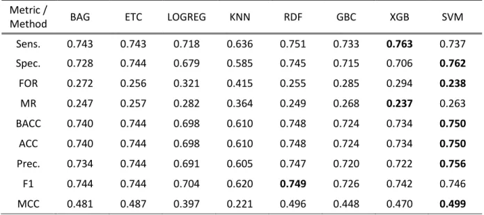
To select the methods for base and meta-classifiers, we examined the performance of eight different machine learning methods, BAG, ETC, LOGREG, KNN, RDF, GBC, XGB and SVM on the benchmark dataset using 10-fold CV. The performance comparison of the classifiers is shown in Table 2.
Table 2: Comparisons of various machine learning algorithms on the benchmark dataset using 10-fold CV.
Best score values are bold faced.
Table 2 shows that the optimized SVM with RBF-kernel provides the highest performance in terms of specificity, fall out rate, balanced accuracy, accuracy, precision, and MCC, among all the classifiers examined in this application. Moreover, the sensitivity and miss rate is highest for the XGB and F1 score is highest for RDF. Similarly, it is evident that the performance of tree-based ensemble methods, BAG, ETC, RDF, GBC, and XGB are close to SVM.
Metric /
Method BAG ETC LOGREG KNN RDF GBC XGB SVM
Sens. 0.743 0.743 0.718 0.636 0.751 0.733 0.763 0.737 Spec. 0.728 0.744 0.679 0.585 0.745 0.715 0.706 0.762 FOR 0.272 0.256 0.321 0.415 0.255 0.285 0.294 0.238 MR 0.247 0.257 0.282 0.364 0.249 0.268 0.237 0.263 BACC 0.740 0.744 0.698 0.610 0.748 0.724 0.734 0.750 ACC 0.740 0.744 0.698 0.610 0.748 0.724 0.734 0.750 Prec. 0.734 0.744 0.691 0.605 0.747 0.720 0.722 0.756 F1 0.744 0.744 0.704 0.620 0.749 0.726 0.742 0.746 MCC 0.481 0.487 0.397 0.221 0.496 0.448 0.470 0.499
27
Figure 5: Illustration of the framework of the final predictor, StackCBPred, which is principally the Model-1 with another version of SVM in the meta layer.
28
The balanced accuracy of these tree-based methods differs from each other and SVM only by about 1 to 4%. However, the balanced accuracy of LOGREG and KNN are 7.31% and 22.79% lower than the SVM, respectively. Moreover, the learning principles of LOGREG, KNN, and SVM are different from each other.
Following the guidelines of base-classifier selection based on different underlying principles, we initially selected SVM, LOGREG, and KNN as three of the base classifiers. Then, we added one tree-based ensemble method out of five methods, BAG, ETC, RDF, GBC, and XGB, at a time as the fourth base-classifier and formulated five different combinations. For all the combinations, the meta-classifier is SVM. Out of five combinations, we present the performance of the top three combinations namely Model-1, Model-2, and Model-3 in Table 4.
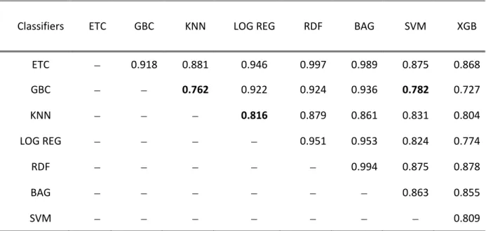
Moreover, we created an additional stacked model following the guidelines of base-classifier selection based on low Pearson correlation coefficient. We computed the Pearson correlation coefficient (ρ) between the two sets of probabilities given by two classifiers using equation (1).
= ∑ 𝑋𝑌
√∑ 𝑋2∑ 𝑌2 (1)
The principle of stacking states that it is preferable to use learners that are weakly correlated in the first-stage to obtain better performance at the second-stage [21]. To select weakly correlated methods, we performed a pair-wise correlation analysis of the residue-wise probabilities between the classifiers. To obtain residue-wise probabilities, the classifiers were trained on benchmark dataset and the probabilities for each residue in the TS49 test set was obtained through an independent test. The results of these correlations are shown in Table 3.
29
Since the SVM was found to be the top performing method from the above comparison between different classifiers, it was selected as a meta-classifier to create the fourth
Table 3: Pair-wise correlation analysis of the probability distribution given by the base-classifiers on TS49.
Classifiers ETC GBC KNN LOG REG RDF BAG SVM XGB ETC − 0.918 0.881 0.946 0.997 0.989 0.875 0.868 GBC − − 0.762 0.922 0.924 0.936 0.782 0.727 KNN − − − 0.816 0.879 0.861 0.831 0.804 LOG REG − − − − 0.951 0.953 0.824 0.774 RDF − − − − − 0.994 0.875 0.878 BAG − − − − − − 0.863 0.855 SVM − − − − − − − 0.809
Identified least pair-wise correlation scores are bold faced.
combination (i.e., Model-4). Next, the method which is least correlated with SVM was identified. From Table 3, we can see that the SVM is least correlated with the GBC with a correlation coefficient of 0.782. Thus, GBC was selected as the first base-classifier. Consequently, the next method which is least correlated with GBC was identified. Again, from Table 3, we found that GBC is least correlated with XGB. However, as both XGB and GBC are based on boosting principle, instead of selecting XGB, next least correlated method was identified. The next least correlated method to GBC was found to be KNN with a correlation coefficient of 0.762. Thus, the KNN was selected as the second base-classifier. Successively, the least correlated method to KNN was identified. Table 3 shows that the least correlated method to KNN excluding GBC and XGB is
30
LOGREG with a correlation coefficient of 0.816. The GBC and XGB were excluded because GBC was already selected as one of the base-classifier and XGB follows the same principle of boosting as GBC.
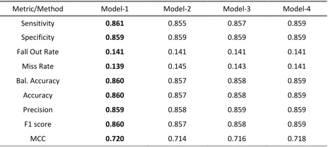
Finally, with the above approach GBC, KNN and LOGREG were selected as base-classifiers to create Model-4. The performance of Model-4 and its comparison with other models is shown in Table 4.
Table 4 shows that the Model-1, which includes SVM, LOGREG, KNN, and ETC as base-classifier and another version of SVM as meta-classifier, provides the highest performance. Thus, we select Model-1 as our final stacking model.
5.1 Performance Comparison on Benchmark Dataset
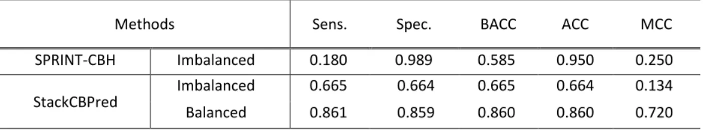
Here, we compute the performance of StackCBPred using 10-fold CV on the benchmark dataset. While performing 10-fold CV the training of the StackCBPred was done using a balanced number of samples whereas, the testing was performed using a balanced as well as an imbalanced number of samples, respectively. Testing using the imbalanced number of samples in 10-fold CV was performed so that the results could be directly compared to SPRINT-CBH. Table 5 shows the performance comparison of StackCBPred and SPRINTCBH. The quantities for all the evaluation metrics for SPRINT-CBH are obtained from Taherzadeh et al. [6].
From Table 5, we observed that the performance of SPRINT-CBH is biased more towards the negative class (non-carbohydrate binding) because of which the specificity (98.9%) is extremely high and the sensitivity (18%) is extremely low. When the test data is highly imbalanced, it is easy
31
to achieve high overall accuracy (ACC) simply by predicting every test data point as the majority class which is what we can see from the result of SPRINT-CBH in Table 5. Balanced accuracy, which avoids inflated performance estimates on imbalanced datasets would be a proper measure of accuracy.
Table 4: Comparisons of stacked models with a different set of base classifiers on benchmark dataset through 10-fold CV.
Metric/Method Model-1 Model-2 Model-3 Model-4
Sensitivity 0.861 0.855 0.857 0.859
Specificity 0.859 0.859 0.859 0.859
Fall Out Rate 0.141 0.141 0.141 0.141
Miss Rate 0.139 0.145 0.143 0.141 Bal. Accuracy 0.860 0.857 0.858 0.859 Accuracy 0.860 0.857 0.858 0.859 Precision 0.859 0.858 0.859 0.859 F1 score 0.860 0.857 0.858 0.859 MCC 0.720 0.714 0.716 0.718
Best score values are bold faced.
However, the balanced accuracy of SPRINT-CBH was not reported in the literature. We computed the balanced accuracy of SPRINT-CBH by utilizing the expression of balanced accuracy provided in Table 1. Moreover, the main goal of the carbohydrate-binding site prediction is to predict the binding sites accurately. However, due to the low sensitivity of 18%, the SPRINT-CBH bears the risk of not identifying the binding sites accurately. On the other hand, StackCBPred can predict the binding sites more accurately than the SPRINT-CBH based on the sensitivity and balanced accuracy scores as shown in Table 5. The sensitivity of the StackCBPred is 66.5% and 86.1% for the imbalanced and balanced number of samples used in testing through 10-fold CV. Additionally, the balanced accuracy of the StackCBPred is 66.5% and 86% for the
32
imbalanced and balanced number of samples used in testing through 10-fold CV.
The StackCBPred attains 13.68% improvement in balanced accuracy over SPRINT-CBH while tested using the imbalanced test set. These results indicate that StackCBPred can predict the binding sites more accurately compared to the SPRINT-CBH.
Table 5:Comparisons of StackCBPred with SPRINT-CBH on the benchmark dataset.
Methods Sens. Spec. BACC ACC MCC
SPRINT-CBH Imbalanced 0.180 0.989 0.585 0.950 0.250 StackCBPred Imbalanced 0.665 0.664 0.665 0.664 0.134 Balanced 0.861 0.859 0.860 0.860 0.720
5.2 Performance Comparison using Independent Test Datasets
In this section, we further examine the performance of StackCBPred by performing an independent test on two independent test datasets, TS49 and TS88. The TS49 dataset was recently constructed by Taherzadeh et al. [6] to test the performance of carbohydrate-binding site predictor, called SPRINT-CBH. However, the TS88 dataset was collected in this study to further test the robustness of StackCBPred. To test using TS49 and TS88, StackCBPred was first trained on balanced benchmark dataset and simultaneously tested on both the independent test datasets. Table 6 lists the predictive results of StackCBPred and SPRINT-CBH on the TS49 test set.
Table 6 indicates that the StackCBPred outperforms SPRINT-CBH by 42.16% and 80.72% based on sensitivity while, tested on the imbalanced and balanced TS49 test set, respectively.
33
Similarly, StackCBPred attains 2.59% and 22.53% improvement in balanced accuracy over SPRINT-CBH while, tested using imbalanced and balanced TS49 test set, respectively. It is to be noted that the main goal here is to predict carbohydrate-binding sites thus, higher sensitivity is preferable.
The results in Table 6 also indicate that the sensitivity of StackCBPred improves from 55.3% to 70.3% and the balanced accuracy improves from 67.4% to 80.5% while, the number of carbohydrate-binding and non-binding residues are balanced in the TS49 test set. The improved sensitivity of carbohydrate binding sites prediction by StackCBPred on TS49 test set also indicates that StackCBPred predicts binding sites more accurately compared to the SPRINT-CBH predictor. Furthermore, the balanced accuracy measure indicates that the StackCBPred is not biased more towards the majority class. Rather it provides a balanced performance compared to SPRINT-CBH method.
Additionally, the performance of StackCBPred and SPRINT-CBH was further evaluated on the TS88 test set and their prediction results are listed in Table 7. Table 7 shows that the sensitivity of StackCBPred is 334.62% better than SPRINT-CBH. Besides, the miss rate of SPRINT-CBH is 0.870 which is very close to 1. Therefore, the specificity of
Table 6: Comparisons of StackCBPred with SPRINT-CBH on balanced and imbalanced independent test dataset, TS49.
Methods Sens. Spec. BACC ACC MCC
SPRINT-CBH Imbalanced 0.389 0.925 0.657 0.906 0.195 StackCBPred
Imbalanced 0.553 0.795 0.674 0.786 0.159 Balanced 0.703 0.907 0.805 0.805 0.623
34
the SPRINT-CBH is very high i.e., it most of the time predicts the sample point as the majority class (non-carbohydrate-binding) which results into low sensitivity. Additionally, the balanced accuracy of the SPRINT-CBH is 20.74% lower compared to StackCBPred. Thus, these results indicate that StackCBPred predicts a greater number of carbohydrate binding and non-binding residues correctly and therefore is also a balanced predictor of carbohydrate-binding sites.
Table 7: Comparisons of StackCBPred with SPRINT-CBH on imbalanced independent test dataset, TS88.
Methods Sens. Spec. FOR MR BACC MCC
SPRINT-CBH 0.130 0.997 0.003 0.870 0.564 0.257
StackCBPred 0.565 0.797 0.203 0.435 0.681 0.139
Moreover, Figure 6 presents the ROC curves generated by StackCBPred and SPRINTCBH, while the predictions are evaluated on the imbalanced TS88 test set. The ROC curves show the TPR (sensitivity)/FPR (1-specificity) pairs at different classification thresholds. It is evident from the ROC curves that the StackCBPred provides higher TPR compared to SPRINT-CBH at different classification thresholds. Moreover, the AUC score given by StackCBPred is about 1.18% higher than that of SPRINT-CBH.
5.3 Statistical Significance Test
We performed McNemar’s test on TS88 independent test set to provide the statistical significance of our results. We could only perform statistical significance on TS88 test set as the prediction results from SPRINT-CBH web-server on TS49 test set do not match the results mentioned in the paper.
35
Figure 6: Comparison of ROC and AUC scores given by StackCBPred and SPRINT-CBH on
imbalanced independent test dataset, TS88.
The differences in the accuracies that are obtained from SPRINT-CBH web-server and the paper could be an outcome of using TS49 test set for training the SPRINT-CBH web-server model. At first, we set our null and alternate hypothesis. For the null hypothesis, we assume that there is no difference between StackCBPred and SPRINT-CBH predictors whereas, for the alternate hypothesis, we assume that there is a significant difference between StackCBPred and SPRINT-CBH predictors. Then, we prepare two different contingency table and conduct McNemar’s test separately. Finally, depending upon the p-value obtained from the McNemar’s test, we either accept or reject our null hypothesis. The detailed approach is shown below:
36
• Null Hypothesis: There is no difference between StackCBPred and SPRINT-CBH predictors.
•Alternate Hypothesis: There is a significant difference between StackCBPred and SPRINTCBH predictors.
Construction of two different contingency tables:
Table 8: Here, the contingency table is formed by comparing the predicted results of StackCBPred and SPRINT-CBH with actual class labels.
StackCBPred
SPRINT-CBH = Actual Class Label ≠ Actual Class Label
= Actual Class Label 21191 5057
≠ Actual Class Label 273 620
Table 9:Here, the contingency table is formed by comparing the predicted results of StackCBPred and SPRINT-CBH with each other.
StackCBPred
SPRINT-CBH Carbohydrate-Binding Non-Carbohydrate-Binding
Carbohydrate-Binding 485 48 533 (1.96 %)
Non-Carbohydrate-Binding 5282 21326 26608 (98.03 %) 5767 (21.24 %) 21374 (78.7 %) 27141
To perform McNemar’s test, we set an alpha value of 0.05 as the cutoff for significance test and run McNemar’s test on both the contingency table shown above. The McNemar’s test for two different contingency tables above resulted in a p-value of < 0.01 which, is less than 0.05. Therefore, we reject the null hypothesis and accept the alternate hypothesis that there is a significant difference between StackCBPred and SPRINT-CBH.
37
Chapter 6
Conclusions
In this work, we have developed a Stacking-based machine learning predictor, named StackCBPred, for the prediction of protein-carbohydrate binding sites directly from the protein sequence. We collected a benchmark dataset and two independent test datasets of high-resolution carbohydrate binding proteins to train, validate and independently test StackCBPred. Several important evolution-derived, sequence-based and structural features were extracted and chosen in an incremental fashion to find the trained best performing model. In addition, an advanced machine learning technique called stacking was implemented to ensure robust performance. We used incrementally chosen features to train the ensemble of predictors at the first-stage (i.e., base-layer). Then, we combined the output from the base-learners with the original features and used it as an input to the predictor at second-stage (i.e., meta-layer). Eventually, the meta-layer predictor of the StackCBPred achieves a 10-fold CV balanced accuracy and sensitivity of 86.00% and 86.09% respectively, on a balanced benchmark dataset. For the balanced independent test dataset, TS49, StackCBPred attains a balanced accuracy and sensitivity of 80.51% and 70.28%, respectively. Furthermore, for the new imbalanced independent test dataset TS88 introduced in this work, StackCBPred attains a balanced accuracy and sensitivity of 68.46% and 56.39%, respectively. These results allow us to conclude that the stacking technique helps improve the accuracy significantly by reducing the generalization error. Moreover, comparative results highlight that the proposed method, StackCBPred, outperforms the existing method based on both benchmark and independent test
38
datasets. These outcomes help us surmise that the StackCBPred can be effectively used for the rapid annotation of carbohydrate-binding sites directly from the sequence and can provide insight in treating critical diseases.
In the future study, we can further improve the performance of StackCBPred, by employing Genetic Algorithm for the feature selection. Genetic Algorithm reflects the process of natural selection where he fittest individuals (in this case the best performing feature set) are selected for reproduction in order to produce offspring of the next generation. Implementing deep learning for the purpose of prediction can be highly effective which uses a cascade of multiple layers and each successive layer uses the output from previous layer as input similar to stacking where we use output from only the base classifiers as input to the meta classifier.
39
References
1. Shionyu-Mitsuyama, C., et al., An empirical approach for structure-based prediction of
carbohydrate-binding sites on proteins. Protein Engineering, 2003. 16(7): p. 467-478.
2. Fernandez-Alonso, M.d.C., et al., Protein-carbohydrate interactions studied by NMR: from molecular
recognition to drug design. Current Protein and Peptide Science, 2012. 13: p. 816-830.
3. Shin, I., S. Park, and M.r. Lee, Carbohydrate Microarrays: An Advanced Technology for Functional
Studies of Glycans. Chemistry - European Journal, 2005. 11: p. 2894-2901.
4. Sharon, N. and H. Lis, Lectins. 2 ed. 2003, The Netherlands: Springer. 454.
5. Wimmerová, M., et al., Stacking interactions between carbohydrate and protein quantified by
combination of theoretical and experimental methods. PLoS ONE, 2012. 7(10): p. e46032.
6. Taherzadeh, G., et al., Sequence-based prediction of protein–carbohydrate binding sites using support
vector machines. Journal of Chemical Information and Modeling, 2016. 56(10): p. 2115-2122.
7. McKinley, M.P., et al., Human anatomy. Fourth edition ed. 2015, New York, NY: McGraw-Hill
Education.
8. Malik, A. and S. Ahmad, Sequence and structural features of carbohydrate binding in proteins and
assessment of predictability using a neural network. BMC Structural Biology, 2007. 7(1).
9. Brown, A. and M.K. Higgins, Carbohydrate binding molecules in malaria pathology. Current Opinion
in Structural Biology, 2010. 20(5): p. 560-566.
10. François, K. and J. Balzarini, Potential of carbohydrate‐binding agents as therapeutics against
enveloped viruses. Medicinal Research Reviews, 2012. 32: p. 349-387.
11. Raz, A. and S. Nakahara, Biological modulation by lectins and their ligands in tumor progression and
metastasis. Anti-Cancer Agents in Medicinal Chemistry, 2008. 8(1): p. 22-36.
12. Morris, G.M., et al., Automated docking using a Lamarckian genetic algorithm and an empirical
binding free energy function. Journal of Computational Chemistry, 1998. 19(14): p. 1639-1662.
13. Friesner, R.A., et al., Glide: a new approach for rapid, accurate docking and scoring. 1. Method and
assessment of docking accuracy. Journal of Medical Chemistry, 2004. 47(7): p. 1739-1749.
14. Moustakas, D.T., et al., Development and validation of a modular, extensible docking program: DOCK
5. Journal of Computer-Aided Molecular Design, 2006. 20(10-11): p. 601-619.
15. Taroni, C., S. Jones, and J.M. Thornton, Analysis and prediction of carbohydrate binding sites. Protein
Engineering, 2000. 13(2): p. 89-98.
16. Sujatha, M.S. and P.V. Balaji, Identification of common structural features of binding sites in
40
17. Kulharia, M., et al., InCa-SiteFinder: A method for structure-based prediction of inositol and
carbohydrate binding sites on proteins. Journal of Molecular Graphics and Modelling, 2009. 28(3): p. 297-303.
18. Nassif, H., et al., Prediction of protein‐glucose binding sites using support vector machines. Proteins:
Structure, Function, Bioinformatics, 2009. 77(1): p. 121-132.
19. Tsai, K.-C., et al., Prediction of carbohydrate binding sites on protein surfaces with 3-dimensional
probability density distributions of interacting atoms. PLoS ONE, 2012. 7(7): p. e40846.
20. Gromiha, M.M., K. Veluraja, and K. Fukui, Identification and analysis of binding site residues in
proteincarbohydrate complexes using energy based approach. Protein and Peptide Letters, 2014. 21(8): p. 799-807.
21. Shanmugam, N.R.S., et al., Identification and analysis of key residues involved in folding and binding
of protein-carbohydrate complexes. Protein and Peptide Letters, 2018. 25(4): p. 379-389.
22. Deng, L., et al., Boosting prediction performance of protein–protein interaction hot spots by using
structural neighborhood properties. Journal of Computational Biology, 2013. 20(11): p. 878-891.
23. Lei, C. and J. Ruan, A novel link prediction algorithm for reconstructing protein–protein interaction
networks by topological similarity. Bioinformatics, 2013. 29(3): p. 355-364.
24. Rao, V.S., et al., Protein-protein interaction detection: methods and analysis. International Journal of
Proteomics, 2014. 2014.
25. Liang, S., et al., Protein binding site prediction using an empirical scoring function. Nucleic Acids
Research, 2006. 34(13): p. 3698-3707.
26. Iqbal, S. and M.T. Hoque, PBRpredict-Suite: a suite of models to predict peptide-recognition domain
residues from protein sequence. Bioinformatics, 2018: p. bty352-bty352.
27. Lavi, A., et al., Detection of peptide-binding sites on protein surfaces: The first step towards the
modeling and targeting of peptide-mediated interactions. Proteins: Structure, Function, Bioinformatics, 2013. 81(12): p. 2096-2105.
28. Petsalaki, E., et al., Accurate prediction of peptide binding sites on protein surfaces. PLoS
Computational Biology, 2009. 5(3).
29. Taherzadeh, G., et al., Sequence‐based prediction of protein–peptide binding sites using support vector
machine. Journal of Computational Chemistry, 2016. 37(13): p. 1223-1229.
30. Lin, C.-K. and C.-Y. Chen, PiDNA: predicting protein–DNA interactions with structural models.
Nucleic Acids Research, 2013. 41: p. W523-W530.
31. Si, J., et al., MetaDBSite: a meta approach to improve protein DNA-binding sites prediction. BMC