Structure learning of context-specific graphical models

Johan Pensar

Structure Learning of Context-Specific

Graphical Models

Johan P

ensar | Struc

tur

e L

ear

ning of C

ont

ex

t-Specific Graphical M

odels | 2016

ISBN 978-952-12-3412-5

Graphical model

Structure learning

Bayesian network

Markov network

Context-speci

�

c independence

Pseudo-likelihood

Search algorithm

Score function

Bayesian inference

Directed acyclic graph

Non-chordal graph

Label

Probability

Uncertainty

Discrete variable

Joint distribution

Likelihood

Structure Learning of

Context-Specific Graphical Models

Johan Pensar

PhD Thesis in Statistics Mathematics and Statistics Faculty of Science and Engineering

Åbo Akademi University Åbo, Finland, 2016

Supervisor

Professor Jukka Corander,

Department of Mathematics and Statistics, University of Helsinki,

Helsinki, Finland

Reviewers

Assistant Professor Mikko Koivisto, Department of Computer Science, University of Helsinki,

Helsinki, Finland Professor Dan Geiger,

Department of Computer Science, Technion - Israel Institute of Technology, Haifa, Israel

Opponent

Professor Dan Geiger,

Department of Computer Science, Technion - Israel Institute of Technology, Haifa, Israel

ISBN 978-952-12-3412-5 Painosalama Oy ˚

Preface

This thesis concludes the research I have conducted during the years 2012-2016 at the subject of Mathematics and Statistics at ˚Abo Akademi University. During this time, I have not only grown as a researcher, but also as a person. This would not have been possible without the endless support from the people around me. For this, I am truly grateful.

First of all, I would like to thank my supervisor Jukka Corander whose help and support I have always been able to count on, although we have worked in different cities. There are few persons with the same amount of positivity and never-ending enthusiasm, whether is about tackling a research problem or building a “stone bridge” for crossing a melt-water stream in the Swiss alps.

I would also like to direct a special thanks to my colleague and friend Henrik Nyman, the second member of team BAPS, ˚Abo division. It has been a pleasure sharing office and discussing various research and non-research related issues. At this point, it is also in place to thank the friendly staff at Hotel Cepina, the venue of Summer Permafrost 2012-2015, where many of the ideas leading to this thesis were generated and developed.

I would like to thank everybody at the subject of Mathematics and Statistics for the excellent work atmosphere. In particular, I would like to thank G¨oran H¨ogn¨as and Paavo Salminen, who have helped me with all kinds of practical matters during my PhD studies.

I thank all co-authors of the included articles for their contributions. I further thank Mikko Koivisto for reviewing my thesis and Dan Geiger for taking the time to both review and act as opponent.

For their financial support, I gratefully acknowledge the Magnus Ehrnrooth foun-dation, the Finnish Doctoral Programme in Stochastics and Statistics (FDPSS), the Center of Excellence in Optimization and Systems Engineering at ˚Abo Akademi Uni-versity, and ˚Abo Akademi University.

Finally, and most importantly, a big thanks goes to my family and friends. It is safe to say that I would not be where I am today without the support and care from my family. Of course, I also warmly thank my ray of sunshine Heidi whom I can always rely on to brighten my day.

˚

Abo, May 2016

Abstract

The ultimate problem considered in this thesis is modeling a high-dimensional joint distribution over a set of discrete variables. For this purpose, we consider classes of context-specific graphical models and the main emphasis is on learning the structure of such models from data. Traditional graphical models compactly represent a joint dis-tribution through a factorization justified by statements of conditional independence which are encoded by a graph structure. Context-specific independence is a natu-ral genenatu-ralization of conditional independence that only holds in a certain context, specified by the conditioning variables. We introduce context-specific generalizations of both Bayesian networks and Markov networks by including statements of context-specific independence which can be encoded as a part of the model structures. For the purpose of learning context-specific model structures from data, we derive score functions, based on results from Bayesian statistics, by which the plausibility of a structure is assessed. To identify high-scoring structures, we construct stochastic and deterministic search algorithms designed to exploit the structural decomposition of our score functions. Numerical experiments on synthetic and real-world data show that the increased flexibility of context-specific structures can more accurately emu-late the dependence structure among the variables and thereby improve the predictive accuracy of the models.

Sammanfattning

Det grundl¨aggande problemet som behandlas i denna avhandling ¨ar modellering av en h¨ogdimensionell simultan f¨ordelning ¨over en m¨angd diskreta variabler. F¨or detta ¨andam˚al unders¨oker vi klasser av kontextspecifika grafiska modeller och vi fokuserar p˚a inl¨arningen av modellstrukturen fr˚an data. Traditionella grafiska mo-deller utg¨or en kompakt representation av en simultan f¨ordelning genom att faktori-sera f¨ordelningen enligt en graf som ˚aterspeglar antaganden om betingat oberoende. Betingat oberoende har en naturlig generalisering i kontextspecifikt oberoende som endast h˚aller i en viss kontext som best¨ams av de betingande variablerna. Vi in-troducerar kontextspecifika generaliseringar av b˚ade Baysianska n¨atverk och Markov-n¨atverk genom att inkludera kontextspecifika oberoenden som en del av modellstruk-turerna. F¨or inl¨arningen av kontextspecifika modellstrukturer fr˚an data anv¨ander vi oss av resultat fr˚an Bayesiansk statistik f¨or att h¨arleda m˚alfunktioner som bed¨omer trov¨ardigheten av en viss struktur. F¨or att identifiera strukturer med h¨og trov¨ardighet anv¨ands deterministiska och stokastiska s¨okalgoritmer som ¨ar designade att utnyttja strukturen i m˚alfunktionernas faktorisering. Numeriska experiment baserade p˚a syn-tetiska och verkliga data p˚avisar att den f¨orb¨attrade flexibiliteten hos kontextspecifika strukturer kan resultera i modeller med h¨ogre prediktiv f¨orm˚aga ¨an traditionella mo-deller.

List of original articles

I Pensar, J., Nyman, H., Koski, T. & Corander, J. (2015). Labeled directed acyclic graphs: a generalization of context-specific independence in directed graphical models. Data Mining and Knowledge Discovery29, 503–533. II Pensar, J., Nyman, H., Lintusaari, J. & Corander, J. (2016). The role of local

partial independence in learning of Bayesian networks. International Journal of Approximate Reasoning69, 91–105.

III Pensar, J., Nyman, H., Niiranen, J. & Corander, J. (2016). Marginal pseudo-likelihood learning of Markov network structures. Submitted.

IV Pensar, J., Nyman, H. & Corander, J. (2016). Structure learning of contextual Markov networks using marginal pseudo-likelihood. Submitted.

Authors’ contributions to Articles I–IV

I The original idea is due to JC. All authors contributed to the development of the model class. JP and HN had the main responsibility in developing the score function. JP had the main responsibility in all remaining aspects of the article. II JP had the main responsibility in all aspects of the article.

III JP had the main responsibility in all aspects of the article.

IV The original idea of applying the marginal pseudo-likelihood on contextual Markov networks is due to JP and JC. All authors contributed to the devel-opment of contextual Markov networks. JP had the main responsibility in all remaining aspects of the article.

In addition to the included articles, the author has co-authored the publications by Nyman et al. (2014, 2015a,b) and Janhunen et al. (2015), which are related to the work covered by this thesis.

Contents

Preface iii

Abstract iv

Sammanfattning v

List of original articles vi

Authors’ contributions to Articles I–IV . . . vi

1 Introduction 1 2 Graphical models 2 2.1 Bayesian networks . . . 3

2.2 Markov networks . . . 5

2.3 Bayesian networks vs. Markov networks . . . 6

3 Context-specific independence in graphical models 7 3.1 Bayesian networks . . . 8

3.2 Markov networks . . . 10

4 Structure learning of graphical models 13 4.1 Score-based learning . . . 13

4.2 Dirichlet as conjugate for the categorical distribution . . . 13

4.3 Marginal likelihood for Bayesian networks . . . 15

4.4 Marginal pseudo-likelihood for Markov networks . . . 17

5 Summaries of the included articles 20 5.1 Article I: Labeled directed acyclic graphs: a generalization of context-specific independence in directed graphical models . . . 20

5.2 Article II: The role of local partial independence in learning of Bayesian networks . . . 20

5.3 Article III: Marginal pseudo-likelihood learning of Markov network structures . . . 21

5.4 Article IV: Structure learning of contextual Markov networks using marginal pseudo-likelihood . . . 21

6 Concluding remarks and future research 23

1

Introduction

Probabilistic models provide a general tool for modeling real-world systems where there is a significant amount of uncertainty involved. In particular, in this thesis we consider (probabilistic) graphical models, which are used for compactly modeling complex joint distributions over a set of discrete variables. A compact representation of a potentially very high-dimensional distribution is achieved by exploiting structure in the distribution in the form of statements of conditional independence, which are naturally encoded by a graph structure. Characterized by the type of graph, the two most common families of graphical models are Bayesian networks and Markov networks, which are both considered in this thesis.

Graphical models have received considerable attention by the statistics and com-puter science community during the last few decades (Cowell et al., 1999; Koller & Friedman, 2009; Koski & Noble, 2009; Lauritzen, 1996; Pearl, 1988; Whittaker, 1990, among others). As a result of their generic applicability, graphical models have been applied in various fields and applications such as medical diagnosis, computer vision, analysis of genetic data, speech recognition, credit risk evaluation, computer security, and protein contact prediction.

Despite their wide adoption, the conditional-independence-based restrictions as-sociated with traditional graphical models have been recognized to be unnecessarily coarse in certain situations. This observation has led to the development of more flex-ible models (Boutilier et al., 1996; Chickering et al., 1997; Corander, 2003; Friedman & Goldszmidt, 1996; Geiger & Heckerman, 1996; Højsgaard, 2003; Poole & Zhang, 2003). In particular, Boutilier et al. (1996) formalized the notion of context-specific independence (CSI) as a natural generalization of conditional independence. By in-cluding CSI into the graphical model framework, it is possible to obtain more accurate model structures which still enjoy a sound independence-based interpretation.

One of the main challenges related to graphical models is learning the model structure from data. This task is very demanding for several reasons, for example, the number of possible structures is extremely large. Still, from a user-perspective it is an important problem since the mere existence of complex models is of limited practical use, if they cannot be automatically and reliably learned from data. For this reason, there has been much research related to learning of graphical models (for an overview, see Koller & Friedman, 2009).

The main goals of the four articles included in this thesis are to generalize the con-cept of CSI in graphical models, develop efficient structure learning methods inspired by Bayesian statistics, and study learning of the proposed model classes in numerical experiments on both synthetic and real-world data. The introductory part of the the-sis gives a brief overview of the work covered by the included articles in the context of related research. We begin in Section 2 by introducing the concept of graphical models and discussing the fundamental properties of both Bayesian networks and Markov networks. In Section 3, we introduce the notion of CSI and show how it can be included in the considered model classes as part of the model structures. In Section 4, we consider the structure learning problem by deriving score functions based on results from Bayesian statistics. In Section 5, we provide summaries of the included articles and discuss their contributions to the research field. Finally, in Section 6, we provide some concluding remarks and discuss potential future research.

2

Graphical models

We consider a set ofddiscrete random variablesX ={X1, . . . , Xd}. Each variableXj

takes on values from a finite set of outcomes represented byXj ={0,1, . . . , rj−1}.

We let V ={1, . . . , d} denote the indices of the variables. For a subsetS ⊆ V, we denote the corresponding variables by XS. We use p(X) to denote the distribution

over X, whereasp(x) is shorthand for the probabilityp(X=x).

The purpose of graphical models is to represent a joint distribution overX in an efficient and compact manner. Even in the case of binary variables, a naive represen-tation requires 2d_{−1 free parameters to specify a joint distribution overdvariables. It}

is easy to realize that such a representation quickly becomes impractical as the num-ber of variables is increased. To overcome this problem, graphical models break down the joint distribution into smaller more manageable parts by exploiting statements of

conditional independence.

Definition 1. Conditional Independence

LetA, B,S be three disjoint subsets ofV. We say thatXA is conditionally

indepen-dent ofXB givenXS if

p(xA|xB, xS) =p(xA|xS)

holds for all (xA, xB, xS)∈ XA× XB× XS wheneverp(xB, xS)>0. This is denoted

by

XA⊥XB |XS.

If S = ∅, then XA⊥ XB is reduced to marginal independence between the two sets

of variables.

To illustrate how conditional independence can be used in practice, consider the joint distribution over three binary variablesX ={X1, X2, X3}. Using the chain rule,

the distribution can be factorized according to

p(X1, X2, X3) =p(X1)p(X2|X1)p(X3|X1, X2). (1)

Considering each factor individually, we need 1 + 2 + 4 = 7 free parameters to specify the joint distribution. Now, assume that

X2⊥X3|X1. (2)

As stated in Definition 1, the last factor in (1) can be simplified accordingly such that

p(X1, X2, X3) =p(X1)p(X2|X1)p(X3|X1),

whereX2no longer affects the conditional distribution ofX3givenX1. The required

number of free parameters is now reduced to 1 + 2 + 2 = 5.

In the example above, the computational savings might seem negligible, however, when considering tens or even hundreds of variables, it would no longer be practi-cally possible to model the joint distribution without simplifying assumptions. In such situations, it is no longer practical to represent the dependence structure among the variables in the form of a list of independence statements. Instead, the depen-dence structure of a graphical model is represented by a graph structure. The graph consists of nodes (or vertices) representing variables and edges representing direct dependences among the variables. On the other hand, lack of edges represents state-ments of conditional independence. The graph offers an intuitive way of illustrating the dependence structure to a human user. Moreover, it also enables use of graph

4 5 2

6

1 3

Figure 1: A DAG over six nodes.

theory when designing algorithms for learning and performing inference in graphical models.

There are two main families of graphical models; Bayesian networks (directed graphical models) and Markov networks (undirected graphical models). In this the-sis, both types are considered. More specifically, Articles I–II consider Bayesian net-works, while Articles III–IV consider Markov networks. A brief overview of the basic properties of each model class is given next. For a more detailed review of the theory of graphical models, see for example Koller & Friedman (2009).

2.1

Bayesian networks

The basis of the Bayesian network formulation is adirected acyclic graph (DAG). We denote a DAG byG= (V, E), whereV ={1, . . . , d} is a set of nodes corresponding to the variables and E is a set of directed edges between the nodes such that (i, j) denotes a directed edge from nodeito nodej. The edge set must satisfy theacyclicity

property, which means that starting from a node it is not possible to return to that node by following the direction of the edges. The parents of a nodej are all nodes from which there is a directed edge to j, that is, pa(j) = {i ∈ V : (i, j)∈ E}. A nodej is called adescendant of nodei, if it can be reached from nodeifollowing the direction of the edges. Atrail is a sequence of nodes for which each pair of consecutive nodes are connected by an edge. As is typical in the graphical model literature, the terms node and variable are occasionally used interchangeably. An example of a DAG over six nodes is found in Figure 1.

In addition to the graph component, a Bayesian network specifies a joint distribu-tion over the variables. The distribudistribu-tion must satisfy the condidistribu-tional independence assumptions encoded by the DAG. These assumptions can be compactly characterized by the directed local Markov property. It states that each variable is conditionally independent of its non-descendants given its parents. Consequently, a DAG implies a factorization of the joint distribution according to

p(X1, . . . , Xd) = d

Y

j=1

p(Xj |Xpa(j)),

which is known as the chain rule for Bayesian networks (Koller & Friedman, 2009, p. 62). For example, the factorization according the DAG in Figure 1 is

p(X1, . . . , X6) =p(X1)p(X2|X1)p(X3|X2)p(X4)p(X5|X1,2)p(X6|X3,5).

The joint distribution of a Bayesian network is thus broken down over the nodes into localconditional probability distributions (CPDs). Consequently, the probability of a joint configuration is simply determined by a product of factors, where each factor corresponds to a conditional probability of a variable given its parents. The basic,

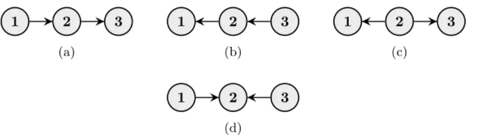
1 2 3 (a) 1 2 3 (b) 1 2 3 (c) 1 2 3 (d)

Figure 2: Possible connections in a Bayesian network: (a)–(b) chain connection, (c)

fork connection, and (d)collider connection.

and perhaps most common, way of specifying the CPDs is in the form ofconditional probability tables (CPTs), which simply list the CPDs such that each row in the table represents a distinct parent configuration.

In addition to the local independences, a Bayesian network encodes a collection of non-local independences which can be derived from the local independences, how-ever, such a derivation can be very cumbersome. Instead, non-local conditional in-dependences can be verified directly from the graph by a sound procedure known as

d-separation. When using d-separation, probabilistic influence should be considered as information flowing through the graph.

To illustrate d-separation and the fundamental properties of Bayesian networks, we look at the possible ways two nodes can be indirectly connected via a third node. The four possible connections are illustrated in Figure 2. Connections 2(a)–(c) are equivalent in the sense that information can pass between nodes 1 and 3 through node 2 if X2 is not observed, while the flow is blocked by node 2 ifX2 is observed. This

corresponds to nodes 1 and 3 being d-separated by node 2, which implies that the conditional independence statement

X1⊥X3|X2

holds for graphs 2(a)–(c). In contrast, the collider connection in Figure 2(d) works in the opposite manner, that is, information can pass through node 2 only if X2 is

observed, while the flow is blocked by node 2 ifX2is not observed. This corresponds

to nodes 1 and 3 being d-separated by the empty set, which implies that the marginal independence statement

X1⊥X3

holds for this graph, however, since nodes 1 and 3 are not d-separated by node 2, the former conditional independence is not implied by the graph. This is known as con-ditional dependence. The same reasoning as above carries over to more complicated graphs where there are more than one trail between a pair of nodes. More formally, a trail is referred to as active givenS if all fork and chain nodes in the trail do not belong toS and for each collider node in the trail, either the collider node itself or one of its descendants belongs to S. Then, two nodesiandj are d-separated byS, implying that

Xi⊥Xj|XS,

if there is no active trail betweeniandj givenS.

The collider connection is also known as av-structureand is a fundamental feature that separates Bayesian networks from undirected models. To further explain its behavior, we use a classic example from the Bayesian network literature (Pearl, 1988). Consider the graph in Figure 2(d). LetX2represent a newly installed burglar alarm,

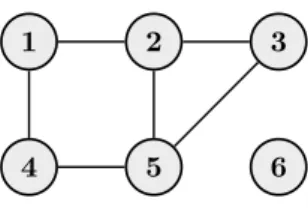
4 5 6

1 2 3

Figure 3: An undirected non-chordal graph over six nodes.

which reliably detects burglary, represented byX1. However, the alarm tends to go

off also in case of an earthquake, represented byX3. There are now two possible and

marginally independent causes that increase the probability of the alarm going off. Say that we are given information that the alarm has gone off, however, we also hear on the radio that there has been an earthquake in the area of the house. Since the knowledge of the earthquake in a sense explains the alarm going off, the alternative cause (burglary) is rendered less likely to have happened. This phenomenon is known asexplaining away.

Since graphs 2(a)–(c) encode the same dependence structure, they are said to belong to the same Markov equivalence class. In terms of modeling a distribution, they are all equivalent in the sense that they represent the same set of distributions.

2.2

Markov networks

The dependence structure of a Markov network is represented by an undirected graph. We use the same graph notation G = (V, E) as in the previous section with the difference that an undirected edge between nodeiandjis denoted by{i, j}. Aclique

C in a graph is defined as a subset of nodes for which all pairs of nodes are connected by an edge. A clique is defined as maximal if no additional node can be added to the clique without violating the clique criterion. TheMarkov blanket of a node j is denoted by mb(j) and defined as all nodes which are connected toj by an edge. A

cycle is a sequence of nodes that starts and ends with the same node and each pair of consecutive nodes are connected by an edge. A graph is said to bechordal if all cycles that contain four or more nodes have achord, that is, an edge that is not part of the cycle but connects two nodes in the cycle. An example of an undirected graph over six nodes is found in Figure 3. This particular graph is non-chordal due to the chordless cycle 1−2−5−4−1.

Similar to a Bayesian network, a Markov network specifies a joint distribution through a set of parameters associated with the undirected graph. However, in con-trast to a Bayesian network, the parameters do not in general correspond to condi-tional probabilities or even probabilities, making them less intuitive. A common way of representing the joint distribution of a Markov network is through a factorization over the maximal cliques in the graph in terms of clique factors (see equation (2.1) of Article III). Another approach is to assume a positive distribution and represent the distribution in terms of a log-linear model

logp(x1, . . . , xd) =

X

A⊆V

φA(x),

where theφ-terms are real-valued coordinate projection functions, such thatφA(x) =

φA(xA). In a graphical log-linear model, the φ-terms satisfy the graph related

con-straint

Furthermore, in order to avoid an over-parameterization, theφ-terms are also defined such that

φA(xA) = 0 ifxj= 0 for anyj∈A. (4)

As an example, the log-linear parameterization associated with the graph in Figure 3 is

logp(x1, . . . , x6) =φ∅+φ1(x) +φ2(x) +φ3(x) +φ4(x) +φ5(x) +φ6(x)

+φ1,2(x) +φ1,4(x) +φ2,3(x) +φ2,5(x) +φ3,5(x) +φ4,5(x)

+φ2,3,5(x).

As specified by restriction (3), no φ-term covers pair of nodes that are not in the edge set of the graph. For more details regarding the log-linear parameterization, see Whittaker (1990).

Similar to Bayesian networks, the graph of a Markov network encodes a depen-dence structure in terms of statements of conditional independepen-dence. The dependepen-dence structure can be characterized by the following Markov properties:

1. Pairwise Markov property: Xi⊥Xj|XV\{i,j} for all{i, j} 6∈E.

2. Local Markov property: Xi⊥XV\{mb(i)∪i}|Xmb(i)for alli∈V.

3. Global Markov property: XA ⊥ XB | XS for all disjoint subsets A, B, S ofV

such thatSseparatesAfromB.

The above properties are proven to be equivalent under the assumption of positivity of the joint distribution (Lauritzen, 1996). Note that the global Markov property is the undirected analogue of the d-separation criterion, however, here AandB are separated by S, if all paths betweenAandB pass throughS.

2.3

Bayesian networks vs. Markov networks

Bayesian networks and Markov networks are in many respects similar. The end goal of both is to represent a joint distribution through a factorization justified by statements of conditional independence which are encoded by a graph. Conditional independences in either model can be verified directly from the graph through the use of separation criteria. The dependence structure encoded by an undirected graph is easier to interpret and perhaps more intuitive. On the other hand, the param-eterization of a Bayesian network is more advantageous due to its “true” factoriza-tion. In comparison, the parameters of a (non-chordal) Markov network are connected through a normalizing constant known as the partition function, which corresponds to the φ_∅-term in the log-linear parameterization. The fundamental difference between Bayesian networks and Markov networks is that they can encode different depen-dence structures; Bayesian networks can represent conditional dependepen-dences through v-structures, whereas Markov networks can represent cyclic dependences. Still, the two model classes partially overlap since, for each chordal undirected graph, there is a corresponding class of Markov equivalent DAGs encoding the same dependence structure. In the end, each model class has its own strengths and weaknesses, and hence, which class is better suited for modeling a particular problem depends on the application in question.

3

Context-specific independence in graphical

mod-els

It has been noticed by several authors that conditional independence alone can in some situations be unnecessarily stringent for modeling real-world phenomena. In an attempt to loosen the restrictions associated with traditional graphical models, the notion ofcontext-specific independence (CSI) has emerged (Boutilier et al., 1996; Corander, 2003; Friedman & Goldszmidt, 1996; Højsgaard, 2003; Poole & Zhang, 2003). CSI is a natural generalization of conditional independence and it was formal-ized by Boutilier et al. (1996) for the purpose of capturing regularities in the CPTs of Bayesian networks.

Definition 2. Context-Specific Independence

Let A, B, C, S be four disjoint subsets ofV. We say that XA is contextually

inde-pendent of XB givenXS and the contextXC =xC if

p(xA|xB, xC, xS) =p(xA|xC, xS)

holds for all(xA, xB, xS)∈ XA× XB× XS wheneverp(xB, xC, xS)>0. This will be

denoted by

XA⊥XB|xC, XS.

When comparing Definition 1 and 2, it is easy to realize that CSI is a more specific form of conditional independence in the sense that it only holds in part of the outcome space of the conditioning variables. In particular, we have the equivalence

XA⊥XB|xC, XS for allxC ∈ XC ⇔XA⊥XB|XC, XS.

To illustrate the concept of CSI in practice, we return to our simple example in Section 2 concerning the factorization (1) of the joint distribution over three binary variables. However, instead of the conditional independence assumption (2), assume that

X2⊥X3|X1= 1 andX26⊥X3|X1= 0.

This gives us a factorization of the joint distribution according to

p(X1, X2, X3) = (

p(X1)p(X2|X1)p(X3|X1, X2), ifX1= 0 p(X1)p(X2|X1)p(X3|X1), ifX1= 1

, (5)

whereX2no longer affects the conditional distribution ofX3given the contextX1= 1.

The number of free parameters required to specify the distribution is reduced by one, from 1 + 2 + 4 = 7 to 1 + 2 + 3 = 6. If we were to only consider conditional inde-pendence, the above CSI statement could not be accounted for in the factorization. Consequently, by exploiting statements of CSI, it is possible to more accurately model a joint distribution without inducing redundant parameters.

One of the main goals of this thesis is to generalize the concept of CSI in graphical models, including both Bayesian networks (Article I) and Markov networks (Article IV). A brief overview of the introduced model classes and the theory surrounding them is given next. For more details, the reader is referred to the articles and other works referenced in the text.

2 3 1 (a) 2 p3 1 p1 p2 1 0 0 1 (b)

Figure 4: (a) A DAG and (b) a CSI-tree of node 3, which together represent the dependence structure corresponding to the factorization in (5).

3.1

Bayesian networks

The conditional independence assumptions made by a Bayesian network enable mod-eling high-dimensional joint distributions through node-wise CPDs. Still, the number of parameters required to specify a traditional CPT of a node j,

(|Xj| −1)· |Xpa(j)|= (rj−1)·

Y

i∈pa(j) ri,

may in some scenarios become overwhelming, since it grows exponentially with the number of parents. In order to counteract the rapid growth in the number of param-eters, use of local CSI statements has been proposed and investigated by numerous authors (Boutilier et al., 1996; Friedman & Goldszmidt, 1996; Poole & Zhang, 2003). By local we refer to a statement concerning the relation between a node and its parents in the form of

Xj⊥Xpa(j)\C |xC whereC ⊂pa(j) (Definition 3, Article I). (6)

Local CSI statements are particularly well-suited for the Bayesian network param-eterization since they imply that certain corresponding CPDs are identical. More specifically, they imply that

p(Xj |xpa(j)\C, xC) =p(Xj|x0pa(j)\C, xC)

for allxpa(j)\C, x0pa(j)\C ∈ Xpa(j)\C. Since identical CPDs need only be specified once,

the number of necessary model parameters can be reduced accordingly. This can be viewed as partitioning the outcome space of the parents into classes of configurations such that the conditional distribution of the node is invariant for parent configurations belonging to the same class.

To illustrate and capture local CSI statements, Boutilier et al. (1996) proposed using decision trees, here referred to as CSI-trees. The internal nodes in a CSI-tree are made up of the parents of the considered node, and the leaves represent distinct CPDs. By starting from the root and traversing down the tree until reaching a leaf, one obtains a context specifying a class in the partition of the parent outcome space. Any parents not included in the context are rendered contextually independent of the node given the context. For example, the complete DAG in Figure 4(a) and the CSI-tree over node 3 in Figure 4(b) together represent the factorization in (5). This representation thus requires a collection of CSI-trees in combination with a DAG. In Article II, we investigate the use of CSI-trees and similar graph structures. An

X1= 0 2 3 1 X1= 1 2 3 1 (a) 2 3 1 X1=1 (b)

Figure 5: (a) A Bayesian multinet and (b) an LDAG, which both represent the dependence structure corresponding to the factorization in (5).

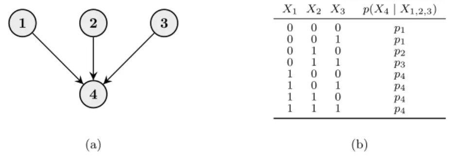
4 2 1 3 (a) X1 X2 X3 p(X4|X1,2,3) 0 0 0 p1 0 0 1 p1 0 1 0 p2 0 1 1 p3 1 0 0 p4 1 0 1 p4 1 1 0 p4 1 1 1 p4 (b)

Figure 6: (a) A DAG over four nodes and (b) an example of a CPT of node 4.

native representation was proposed by Geiger & Heckerman (1996), who introduced the concept of Bayesian multinets which can represent asymmetric independence, such as CSI, by using multiple networks. For example, the dependence structure in Figure 4 can be represented by the two context-specific DAGs in Figure 5(a).

Inspired by the work of Corander (2003), in Article I we introduce labeled di-rected acyclic graphs (LDAGs)which specify the dependence structure using a single graphical structure. In an LDAG, each edge is assigned a label that specifies a set of contexts for which the influence of that edge “vanishes” according to local CSI statements. For example, the LDAG in Figure 5(b) captures the information from the graphs in 5(a) in a single structure. For clarity, the variable specifying the label is here explicitly specified. Given a fixed ordering of the nodes, this is not necessary since the variables specifying a label are all parents except the one that is part of the edge.

To further illustrate the concept of LDAGs, consider the DAG in Figure 6(a) and the associated CPT of node 4 in Figure 6(b). We assume that all variables are binary. A closer examination of the CPT reveals several identical CPDs which can be explained by CSI. Firstly, we see that (0,0,0) and (0,0,1) induce the same conditional distribution. This corresponds to the local CSI statement

X4⊥X3|X1= 0, X2= 0.

Furthermore, we see that the conditional distribution remains the same in the context

X1= 1 regardless of the values ofX2andX3. This corresponds to X4⊥ {X2, X3} |X1= 1.

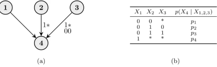
4 2 1 3 1∗ 00 1∗ (a) X1 X2 X3 p(X4|X1,2,3) 0 0 * p1 0 1 0 p2 0 1 1 p3 1 * * p4 (b)

Figure 7: (a) An LDAG capturing the regularities in the CPT in Figure 6(b) and (b) the corresponding reduced CPT.

can be taken into account by the LDAG in Figure 7(a). Here we use a more compact notation where the label 1∗ represents the set{1} × {0,1}= {(1,0),(1,1)}. Figure 7(b) contains the corresponding reduced CPT which has been constructed according to the labels such that each row represents a class in the partition of the parent outcome space:

0 0∗={(0,0,0),(0,0,1)},

0 1 0 ={(0,1,0)},

0 1 1 ={(0,1,1)},

1∗ ∗={(1,0,0),(1,0,1),(1,1,0),(1,1,1)}.

For more details on how the reduced CPT (or partition) is constructed with respect to an LDAG, see Section 2.1 of Article I.

The regularities in the above CPT are again consistent with a CSI-tree, however, this is not always the case. In contrast, LDAGs are general representations of CSI in the sense that they can represent any collection of CPD regularities consistent with CSI. Consequently, any Bayesian network with CSI-trees can be represented by an LDAG, whereas all LDAGs cannot be represented using CSI-trees. For an example of this, see Figure 5 of Article I.

In Section 2.2 of Article I, the properties of LDAGs are investigated more in detail and corresponding context-specific versions of d-separation and Markov equivalence are introduced and discussed. As an example of different LDAGs representing the same dependence structure, change the direction of the edge between nodes 2 and 3 in Figure 5(b).

3.2

Markov networks

Although originally formalized in the context of Bayesian networks, the notion of CSI has also been investigated as a means for improving the flexibility of Markov networks (Corander, 2003; Højsgaard, 2003; Nyman et al., 2014, 2015a,b). In par-ticular, Corander (2003) introduced the class oflabeled graphical models, which later was investigated further by Nyman et al. (2014, 2015a) who developed the subclasses ofdecomposable stratified graphical modelsandstratified graphical models. Compared to the original work by Corander (2003), certain restrictions were imposed on the stratified graphical model classes in order to facilitate the model learning process. In Article IV, we introduce the class ofcontextual Markov networks which in principle is equivalent to the class of labeled graphical models, however, it is defined in a slightly different manner due to an observation made in Nyman et al. (2015a).

Similar to LDAGs, each edge in a contextual Markov network is assigned a context (or label) which is now specified by the common neighbors of the edge nodes. The

2 3 1

X1=1

Figure 8: Labeled undirected graph encoding the dependence structure of a contextual Markov network.

common neighbors with respect to an undirected edge{i, j}are denoted and defined by cn(i, j) = mb(i)∩mb(j). An edge context specifies values for which the direct dependence encoded by the edge “vanishes” according to local CSI statements which are now of the form

Xi⊥Xj |xcn(i,j), XV\{cn(i,j)∪{i,j}} (Definition 2, Article IV). (7)

Using the common neighbors to specify an edge context is proven to be a natural condition. In Section 2.2 of Article IV, we show that the generality of contextual Markov networks would not be increased if allowing an edge context to be specified by supersets or subsets of the common neighbors.

The edge contexts can be illustrated by labeled undirected graphs using a similar notation as for LDAGs. Following a similar reasoning as Corander (2003) and Nyman et al. (2015a), we show in Proposition 2 of Article IV that CSI statements of the above type correspond to linear restrictions among the log-linear parameters. To illustrate the idea behind the result and at the same time bridge the gap between CSI in Bayesian networks and CSI in Markov networks, we return to our toy network. Consider the labeled undirected graph in Figure 8. Again for clarity, we have explicitly stated that X1 specifies the label although it is clear since node 1 is the common

neighbor of nodes 2 and 3, or using our notation, cn(2,3) = 1. The above labeled graph obviously encodes the same dependence structure as the LDAG in Figure 5(b). The underlying complete graphs are equivalent and, according to (6) and (7), both labels encode the CSI statement

X2⊥X3|X1= 1.

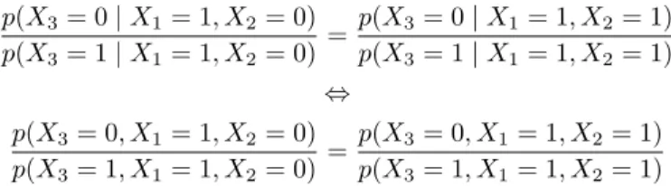
The question is then: How is the above CSI restriction taken into account in the log-linear parameterization? From the LDAG framework, we know that the CSI statement implies that

p(X3|X1= 1, X2= 0) =p(X3|X1= 1, X2= 1).

However, the above restriction can after some reformulation be expressed in terms of joint probabilities: p(X3= 0|X1= 1, X2= 0) p(X3= 1|X1= 1, X2= 0) = p(X3= 0|X1= 1, X2= 1) p(X3= 1|X1= 1, X2= 1) ⇔ p(X3= 0, X1= 1, X2= 0) p(X3= 1, X1= 1, X2= 0) = p(X3= 0, X1= 1, X2= 1) p(X3= 1, X1= 1, X2= 1)

4 5 1 2

3

0

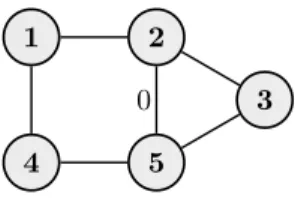
Figure 9: An undirected non-chordal labeled graph over five nodes.

Taking the logarithm of both sides and using the log-linear expansion, we obtain (φ_∅+φ1)−(φ∅+φ1+φ3+φ1,3)

=

(φ_∅+φ1+φ2+φ1,2)−(φ∅+φ1+φ2+φ3+φ1,2+φ1,3+φ2,3+φ1,2,3).

We drop the arguments from the φ-terms since we are dealing with binary variables under assumption (4). After simplification the above equation is reduced to

φ2,3+φ1,2,3= 0,

which elegantly captures the considered CSI. The same reasoning was used in a more general setting to prove Proposition 2 of Article IV which states that a contextual Markov network can be formulated in terms of a log-linear model in which the pa-rameters are being subject to linear restrictions implied by the edge contexts.

As mentioned, the class of contextual Markov networks is basically equivalent to the class of labeled graphical models, except that the definition of edge context (or label) has been modified to remain sound for non-chordal graphs. In previous works (Corander, 2003; Nyman et al., 2014, 2015a), a label was defined to encode CSI statements of the form

Xi⊥Xj |xcn(i,j). (8)

In a chordal graph, the common neighbors are indeed sufficient to cut off any indirect dependences, however, consider the non-chordal graph in Figure 9. Even if the direct dependence between node 2 and 5 is removed and the indirect dependence via 2−3−5 is blocked by nodecn(2,5) = 3, there is still a path 2−1−4−5 along which information can flow, rendering the variables dependent. To address this issue in Article IV, the new definition (7) explicitly refers to the direct dependence by conditioning on the remaining network (cf. pairwise Markov property).

4

Structure learning of graphical models

In this section, we consider one of the main inference tasks related to graphical mod-els, learning the model structure from a set of data. The task of constructing networks manually is at best daunting and in general infeasible due to the complexity of the models. It is therefore of utmost importance to develop efficient learning algorithms that can automatically identify a suitable model from data. From a practical stand-point, developing more expressive model classes is of limited use if the models cannot be learned from data. With this in mind, in addition to developing new and more flexible model classes, the main emphasis of this thesis is on learning the structure of such models.

As will be discussed next, Bayesian networks and Markov networks pose different problems in the learning phase. Moreover, the learning task is already challenging for traditional graphical models and generalizing the models in terms of CSI further complicates the matter. Still, the potential gain of a more flexible model is that it can better emulate a target distribution without inducing redundant parameters.

4.1

Score-based learning

Structure learning methods can roughly be divided into two categories; constraint-based and score-constraint-based. Constraint-constraint-based methods try to infer the dependence struc-ture through a series of separate independence tests that exploit the fundamental independence assumptions associated with the model class. Score-based methods, on the other hand, approach the learning task as an optimization problem over the space of possible model structures. Firstly, this requires a score function by which the plausibility of each structure can be evaluated. Secondly, to find high-scoring networks, this also requires an optimization algorithm since an exhaustive evaluation of the structure space is in general infeasible beyond toy-sized systems. Score-based methods are usually more demanding computationally, however, they tend to be more stable since they adopt a more global approach.

In this thesis, we focus on scored-based methods. The score functions are derived according to a Bayesian view and optimized using both a stochastic algorithm (Article I) and various deterministic algorithms (Articles II–IV). In the coming sections, we focus on the derivation of the score functions and mainly discuss the optimization in terms of how the structure of the scores can be exploited to design efficient search algorithms. For more details on the specific search algorithms, the reader is referred to the included articles.

4.2

Dirichlet as conjugate for the categorical distribution

Before proceeding to discuss the learning methods, we will go through a standard result from Bayesian analysis which is central for the derivation of the Bayesian score functions used in this thesis. The result concerns a special relationship between the categorical and Dirichlet distributions.

Definition 3. Categorical distribution

A categorical distribution over a discrete variableX withr >0possible outcomes and parametersθ= (θ1, . . . , θr), where θ1, . . . , θr >0 andPri=1θi= 1, has the probability

mass function p(X=x(i);θ) =θi fori= 1, . . . , r.

The categorical distribution is a generalization of the Bernoulli distribution (r= 2) and is the most general distribution over an r-way outcome space since the proba-bility of each outcome is separately defined throughθ= (θ1, . . . , θr). If denoting the

outcome by a vector rather than an integer, the categorical distribution is equivalent to a multinomial distribution over a single trial. As a result of this, the categorical distribution is often also referred to as the multinomial distribution in the literature.

Definition 4. Dirichlet distribution

A Dirichlet distribution over r ≥ 2 variables θ = (θ1, . . . , θr) with parameters α =

(α1, . . . , αr), whereαi>0fori= 1, . . . , r, has a probability density function given by

f(θ;α) = Γ( Pr i=1αi) Qr i=1Γ(αi) r Y i=1 θiαi−1 if θ1, . . . , θr >0 and Pr

i=1θi= 1. The density is zero elsewhere.

The Dirichlet distribution is a multivariate generalization of the beta distribution (r= 2). The support of the Dirichlet distribution is the (r−1)-dimensional simplex, which basically is a set of r-dimensional generic discrete probability distributions, that is, categorical distributions.

The reason for the popularity of the Dirichlet distribution in Bayesian statistics is that it is a conjugate prior for the categorical (and multinomial) distribution. A distribution is called a conjugate prior for thelikelihood function if theposterior and

prior distributions belong to the same family of distributions. More specifically, let

xdenote a sample ofni.i.d. observations assumed to have been generated from

X |θ∼Categorical(θ)

and letnidenote the number of times outcomeioccurs in the dataset. The posterior

distributionθ|xis defined as

f(θ|x) = p(x|θ)f(θ)

p(x) , (9)

where p(x|θ) is the likelihood function of the parameters for the given data, in our case given by p(x|θ) = r Y i=1 θ_ini, f(θ) is the prior distribution over the parameters, and

p(x) =

Z

p(x|θ)f(θ)dθ (10)

is the probability of the data, known as themarginal likelihood. Now, assuming that the prior distribution over the parameters is Dirichlet,

θ∼Dirichlet(α1, . . . , αr),

then the corresponding posterior distribution is also Dirichlet,

θ|x∼Dirichlet(α1+n1, . . . , . . . , αr+nr),

where the α’s, known as hyperparameters, have been updated by the counts in the data. In this context, it is easy to realize why the hyperparameters in the Dirichlet prior are also commonly referred to as pseudo-counts.

From a computational perspective, a conjugate prior is very convenient since it results in a closed-form expression for the posterior. Moreover, it allows us to derive a closed-form expression for the marginal likelihood:

p(x) = Γ( Pr i=1αi) Γ(n+Pr i=1αi) r Y i=1 Γ(ni+αi) Γ(αi) . (11)

The above formula is the key result used when deriving the Bayesian score functions at which we look at next. In practice, the logarithm of the above formula is used, since it is computationally more manageable.

4.3

Marginal likelihood for Bayesian networks

The most widely used score for structure learning of Bayesian networks from data is the Bayesian score. By a dataset x, from now on we refer to a complete dataset consisting ofni.i.d. joint observations overdvariables. In the Bayesian approach, a graphGis scored by the unnormalized conditional probability of the graph given a dataset x,

p(G|x)∝p(x|G)p(G),

wherep(x|G) is the marginal likelihood under the given graph andp(G) is the prior probability of the graph.

The key factor of the Bayesian score is the marginal likelihood which, similar to (10), is evaluated by

p(x|G) =

Z

p(x|G, θ)f(θ|G)dθ. (12) We let θjl = (θ1jl, . . . , θrjjl) be the parameters specifying the CPD (in terms of

a categorical distribution) over node j given that the parents have been assigned configurationl. Furthermore, letnijl be the count of the number of times the

corre-sponding family configuration occurs in the data. The likelihood function can then be compactly represented by the product

p(x|G, θ) = d Y j=1 qj Y l=1 rj Y i=1 θnijl_ijl . (13)

Under certain assumptions listed by Heckerman et al. (1995), the above integral can be solved analytically resulting in a closed-form expression (Buntine, 1991; Cooper & Herskovitz, 1992). In particular, one of the key assumptions is parameter indepen-dence, which allows for a factorization of the parameter prior according to

p(θ|G) = d Y j=1 qj Y l=1 f(θjl). (14)

This means that the global integral in (12) can be replaced by a product of local integrals. By further assuming Dirichlet distributions over theθjl’s,

θjl∼Dirichlet(α1jl, . . . , αrjjl),

the local integrals can be solved in an equivalent manner as (11). The marginal likelihood for Bayesian networks is then obtained as the closed-form expression

p(x|G) = d Y j=1 qj Y l=1 Γ(Prj i=1αijl) Γ(njl+ Prj i=1αijl) rj Y i=1 Γ(nijl+αijl) Γ(αijl) , (15)

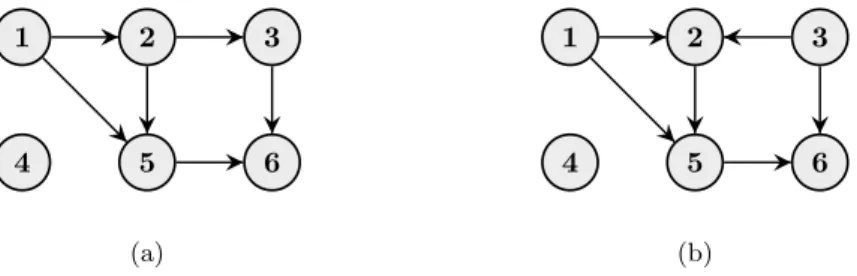
4 5 2 6 1 3 (a) 4 5 2 6 1 3 (b)

Figure 10: Two DAGs, (a) G1 and (b)G2, over six nodes that are identical except

that the direction of the edge between node 2 and 3 is different.

where njl =P rj

i=1nijl. The above expression is easily evaluated once the

hyperpa-rameters have been specified.

In addition to the marginal likelihood, the Bayesian score includes a graph prior,

p(G), through which it is possible to incorporate prior beliefs regarding the graph in terms of, for example, degree of sparsity. To maintain the useful factorization of the final score, the prior must be defined in a way that enables such a factorization. In general, the marginal likelihood as such has empirically been shown to give good results for Bayesian networks with standard CPTs. Therefore, it is quite common to assume a uniform prior over the graph space.

Note that the marginal likelihood factorizes into node-wise marginal conditional likelihoods according to p(x|G) = d Y j=1 p(xj|xpa(j)). (16)

For example, the marginal likelihood for the graph in Figure 10(a) is factorized as

p(x|G1) =p(x1)p(x2|x1)p(x3|x2)p(x4)p(x5|x1,2)p(x6|x3,5).

The factorization property makes the marginal likelihood attractive from a learning perspective. In particular, search algorithms based on local edge changes (add, delete, and reverse edge) exploit this. In order to evaluate a single edge change, it suffices to re-evaluate at most two node-wise scores since the remaining are kept identical and can be re-used from the previous iteration. For example, say that we want to compare the two graphs in Figure 10 which are otherwise identical but the direction of the edge between node 2 and 3 is different. To compare the graphs (under a uniform prior), we calculate the ratio of their marginal likelihoods, known as theBayes factor, which is reduced to

p(x|G1) p(x|G2)

= p(x2|x1)p(x3|x2)

p(x2|x1,3)p(x3)

since the remaining factors cancel out. Given thatG1is our current graph and that

we have stored the values of its node-wise factors, it is sufficient to calculate the two new factors in the denominator in order to evaluate the above expression. Add and delete operations are even simpler to evaluate, since they only affect the local structure of a single node. The search algorithms in Articles I–II are designed to exploit this factorization property.

Another attractive property of the marginal likelihood for Bayesian networks is that it can readily be modified to take CSI and similar local independences into ac-count (Chickering et al., 1997; Friedman & Goldszmidt, 1996). In a similar manner as previous works, we modified the marginal likelihood to cover LDAGs (Article I)

and networks where the CPTs are modeled using various graph-based representations (Article II). The common thing for these generalized networks is that they partition each parent outcome space into classes with invariant CPDs for parent configurations contained by the same class. Consequently, the marginal likelihood can still be evalu-ated by expression (15), however, with the distinction that thel-index now runs over parent classes rather than distinct parent configurations.

While the marginal likelihood works well as such for traditional Bayesian networks, we noticed in Article I that it favored dense LDAGs with large label sets. The complex structures of such models are not only computationally demanding to learn but the models also showed tendencies of overfitting manifested in poor out-of-sample predictive performance. To attend this issue, a tunable prior that penalized inclusion of labels was proposed. The tuning parameter was chosen by a cross-validation-based method. In Article II, the observation in Article I was confirmed in more extensive simulation studies. In this article, we designed a prior that promoted sparsity in terms of the graph structure.

In Articles I–II, we show how to further exploit the structural decomposition of the marginal likelihood when learning parent classes through local changes in an analogous manner as discussed above. Since the marginal likelihood score for a node

j is further factorized over the parent classes,

p(xj|xpa(j)) = qj Y l=1 p(xj |x (l) pa(j)),

it is sufficient to only re-evaluate those classes that have been modified and re-use the scores for the remaining classes from the previous iteration.

4.4

Marginal pseudo-likelihood for Markov networks

Whereas the marginal likelihood can be evaluated in closed form for Bayesian net-works, its calculation poses significant problems for Markov networks. Due to the partition function, likelihood-based scores are in general intractable for non-chordal Markov networks. For this reason, alternative objective functions have been proposed. One of the most popular is perhaps thepseudo-likelihoodintroduced by Besag (1975). In Article III, we introduce themarginal pseudo-likelihood (MPL)as a Bayesian ver-sion of the pseudo-likelihood score.

The pseudo-likelihood approximates the likelihood by a product of conditional likelihoods over each individual node conditional on all other variables or, given a graph, the Markov blankets,

ˆ p(x|G, θ) = d Y j=1 p(xj|xmb(j), θ).

In a similar manner as in the previous section, we use the notationθijl to represent

the conditional probability of variablej being assigned valueigiven that the node’s Markov blanketmb(j) has been assigned configurationl. We modify the definition of the count nijl analogously. Given the modified notation, the pseudo-likelihood of a

graphGcan be expressed as

ˆ p(x|G, θ) = d Y j=1 qj Y l=1 rj Y i=1 θnijl_ijl ,

4 5 2 6 1 3 (a) 4 5 2 6 1 3 1 (b)

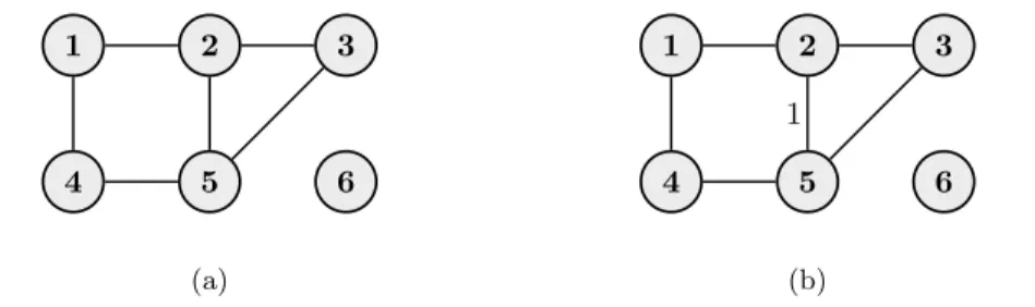
Figure 11: (a) An undirected graph and (b) a labeled undirected graph over six nodes.

which has a striking resemblance to the likelihood in (13). The MPL is obtained by replacing the likelihood in (12) with the pseudo-likelihood. By assuming a similar factorization of the parameter prior as in (14), we can solve the MPL in closed form obtaining a similar expression as in (15), however, the l-index runs over Markov blanket configurations instead of parent configurations. See Section 4.1 of Article III for more details.

It is worth pointing out that the parameter independence assumption made during the derivation of the MPL is justified purely by computational convenience, since it actually violates the properties of a distribution associated with a Markov network. Still, in Theorem 4.1 of Article III, we motivate the MPL from a theoretical standpoint by establishing consistency in the large sample limit, that is, the correct graph will obtain the highest score as the sample size tends to infinity.

Similar to the marginal likelihood for Bayesian networks (16), the MPL factorizes into disconnected marginal conditional likelihoods,

ˆ p(x|G) = d Y j=1 p(xj|xmb(j)).

As an example, the undirected graph in Figure 11(a) is evaluated according to ˆ

p(x|G) =p(x1|x2,4)p(x2|x1,3,5)p(x3|x2,5)p(x4|x1,5)p(x5|x2,3,4)p(x6).

The factorization property makes the MPL an attractive objective function from a computational perspective. Search algorithms based on local changes (add/delete edge) are particularly convenient since a single edge change will modify the Markov blankets of only two nodes. Consequently, only two node-wise scores need to be re-evaluated whereas the remaining scores are kept unchanged and can be re-used from the previous iteration. For more details regarding this, see Sections 4.3 and 5.2 of Article III.

The main reason for imposing restrictions, such as chordality, on the context-specific model classes in Nyman et al. (2014, 2015a) is to facilitate the model learning process. For this purpose, we extended the scope of the MPL in Article IV to also cover contextual Markov networks. In particular, by combining the results of Articles I and III, we showed that the MPL can still be evaluated in closed form for this general class of context-specific Markov networks. The key innovation lies in the observation that the CSI statements of a contextual Markov network can be accounted for by the MPL by partitioning the outcome space of the Markov blankets in a similar manner as the outcome space of the parents in an LDAG. To give an example, consider the labeled graph in Figure 11(b). The label represents the CSI statement

X2⊥X5|X3= 1, X1,4,6.

Under the Markov properties of the given graph, the CSI can be reformulated accord-ing to X2⊥X5|X3= 1, X1,4,6⇔ X2⊥X5|X3= 1, X1 X5⊥X2|X3= 1, X4 ,

where the statements on the right are analogous to local CSI statements in an LDAG where a node’s Markov blanket is thought of as parents. Consequently, the statements on the right can readily be accounted for by the MPL by partitioning the outcome space of the Markov blankets mb(2) = {1,3,5} and mb(5) = {2,3,4} accordingly when evaluating the scores of node 2 and node 5. The scores of the remaining nodes are calculated as regular MPL where each Markov blanket configuration is considered separately. For more details, see Section 3.2 of Article IV.

As for traditional Markov networks, we show in Theorem 1 of Article IV that the resulting MPL-based estimator is consistent in selecting the structure of a contextual Markov network. To avoid the issue of identifying overly dense graphs for limited sample sizes, we propose a tunable prior that penalizes inclusion of context elements (or labels) in a similar fashion as the prior proposed for LDAGs. However, in con-trast to the cross-validation-based approach used in Article I, we use the Bayesian information criterion (BIC) (Schwarz, 1978), which is also a consistent score, for choosing the final model structure from a collection of candidate structures learned under differently tuned priors. The idea behind the approach is that any potential overfitting with respect to the pseudo-likelihood-based MPL will lead to a reduced value on the maximum-likelihood-based BIC score, the numerical experiments showed that the method seems to work quite well in practice. The obvious advantage of using BIC instead of cross-validation is that the maximum likelihood estimates of the log-linear model parameters only need to be calculated once, which is a computationally demanding task due to the partition function.

5

Summaries of the included articles

5.1

Article I: Labeled directed acyclic graphs: a

generaliza-tion of context-specific independence in directed graphical

models

This article introduces the concept of labeled directed acyclic graphs (LDAGs) as a tool for representing context-specific independence (CSI) in Bayesian networks. In contrast to previous proposals, we show that LDAGs can represent general CSI con-straints through a single graph structure. We introduce and discuss several properties of LDAGs in terms of model identifiability and interpretability. To facilitate the inter-pretation of LDAGs, we re-use conditions originally introduced for the class of labeled graphical models (Corander, 2003). Based on the work by Boutilier et al. (1996), we introduce and discuss a context-specific version of the d-separation criterion which can be applied on LDAGs. Finally, we investigate situations where two distinct LDAGs can represent the same dependence structure.

To enable efficient learning of LDAGs from data, we derive a Bayesian score for which the marginal likelihood can be calculated analytically. This is achieved by as-suming an LDAG-based factorization of the Dirichlet prior for the model parameters in a similar manner as Friedman & Goldszmidt (1996). To identify high-scoring struc-tures, we use a stochastic search, developed in Corander et al. (2008, 2006), combined with a deterministic greedy hill-climb method. During the numerical simulations, we noticed that the marginal likelihood alone has a tendency of overfitting by favoring dense LDAGs with large label sets. For this reason, we propose a tunable structure prior which penalizes inclusion of labels. To choose among several candidate values on the tuning parameter, we use a cross-validation-based method.

In our simulations, we use synthetic Bayesian networks based on both a DAG and an LDAG. The quality of an identified structure is assessed by the Kullback-Leibler di-vergence between the true distribution and the approximate model distribution. The numerical experiments show that the models based on LDAGs can outperform tradi-tional Bayesian networks in terms of approximating an actual network distribution, especially when the true network contains CSI.

5.2

Article II: The role of local partial independence in

learn-ing of Bayesian networks

This article further investigates the role of structured conditional probability tables (CPTs) when learning Bayesian networks. We consider models with various degrees of expressiveness, from restrictions consistent with CSI to arbitrary equalities among the conditional probability distributions. To collect all such restrictions under a single notion, we introduce the concept of partial conditional independence. Due to computational advantages, we focus on tree-like CPT structures. In particular, we show that CSI-trees can be extended to capture an additional form of regularities, which are particularly useful for high cardinality variables.

To evaluate the plausibility of the model structures, we modify the Bayesian score from Article I in a similar manner as Chickering et al. (1997). However, in contrast to the label-dependent prior in Article I, we define a structure prior in terms of the DAG alone and do not distinguish between different CPT structures a priori. To identify high-scoring models, we use a deterministic search algorithm which traverses greedily among DAGs using local edge changes. The CPT structures are learned using a greedy hill-climb method that operates in a top-down fashion.

We perform extensive numerical experiments on both synthetic data generated by benchmark Bayesian networks and real data from a machine learning repository. To assess the quality of the models, we use, among others, a measure of predictive accuracy which is comparable to empirical Kullback-Leibler divergence estimated from observed data. We show that including CPT structures in the learning process may significantly improve the quality of the inferred models for both synthetic and real data. However, we also confirm our observation from Article I in that it is usually necessary to further regulate the marginal likelihood through, for example, a prior over the network structures.

5.3

Article III: Marginal pseudo-likelihood learning of Markov

network structures

This article introduces a new Bayesian-type score function for learning the graph structure of non-chordal Markov networks. Due to the partition function, the Bayesian approach for learning the graph structure from data has been restricted to chordal Markov networks for which the marginal likelihood can be calculated analytically (Dawid & Lauritzen, 1993). Chordality, however, is a rather strong assumption which may be unnatural when modeling real-world phenomena. Therefore, we introduce the marginal pseudo-likelihood (MPL) as a Bayesian version of the pseudo-likelihood (Be-sag, 1975) where graph-specific nuisance parameters are marginalized out.

We show that the MPL can be evaluated in closed form under certain assumptions. We investigate the properties of the MPL as a scoring function and, in particular, we show in Theorem 4.1 that the resulting MPL-based graph estimator is consistent in the large sample limit. We discuss the computational complexity of the MPL and its attractiveness from an optimization perspective. Finally, we also discuss the relationship between MPL and the asymptotically equivalent pseudo-Bayesian information criterion (Csisz´ar & Talata, 2006) and a special class of dependency networks (Heckerman et al., 2001).

For MPL optimization, we design a two-step procedure which can be applied on high-dimensional systems. The first step works as a pre-scan picking out potential edges and the second step performs a greedy hill-climb on a restricted graph space determined by the first step. We perform extensive experiments comparing our MPL method to several competing methods on both synthetic and real-world networks with known graph structure. The performance of the methods is evaluated by the resemblance between the inferred and true graph structure as quantified by the Ham-ming distance. Overall, the MPL method outperforms the competing methods at a comparable learning time.

5.4

Article IV: Structure learning of contextual Markov

net-works using marginal pseudo-likelihood

This article introduces a general class of context-specific Markov networks, called contextual Markov networks. Context-specific Markov networks were originally in-troduced by Corander (2003) and later further developed by Nyman et al. (2014, 2015a). One of the main challenges with these models has been the task of learn-ing the model structure from data. For this reason, Nyman et al. (2014) introduced restrictions on the models in the form of chordality and certain context-related condi-tions, which together allow for the marginal likelihood to be evaluated in closed form. In Nyman et al. (2015a), the restrictions on the context structure were lifted making the models more flexible, but at the same time likelihood-based scores intractable in

practice for larger systems. In this article, we lift the restriction of chordality and consider a fully general setting in terms of CSI, as originally proposed by Corander (2003).

The main contribution of this article is extending the scope of MPL to contextual Markov networks by combining the results from Articles I and III. We show that the MPL can still be evaluated in closed form, since the considered CSI statements can be accounted for in a similar manner as local CSI statements in LDAGs. Furthermore, we show that the MPL-based estimator for contextual Markov network structures is consistent in the large sample limit. To avoid the issue of overfitting, we propose a similar tunable prior as was used in Article I, however, instead of using cross-validation, we choose the final model according to the Bayesian information criterion (Schwarz, 1978).

To identify high-scoring structures, we design a deterministic greedy hill-climb algorithm. We perform numerical experiments to investigate how the MPL performs in practice on both synthetic and real-world data. The identified structures are pri-marily evaluated by the predictive accuracy of the corresponding models. The model parameters are approximated by the maximum likelihood estimates which are cal-culated by a conjugate gradient ascent technique. Overall, the identified contextual Markov networks show an improved predictive accuracy both in- and out-of-sample compared to traditional Markov networks.

6

Concluding remarks and future research

The notion of CSI has been proposed as a means to generalize probabilistic graphical models such as Bayesian networks and Markov networks. We have further pursued this idea through the concept of context-specific graphical models in which CSI is included as part of the model structure. The main emphasis of this thesis has been on learning such model structures from data. Compared to traditional graphical models, learning the structure of context-specific graphical models is considerably more challenging due to the extremely large space of possible structures. In addition to making the learning task more demanding computationally, we noticed a previously not recognized problem in the form of overfitting if the structure was optimized with respect to the marginal likelihood alone. To fix this issue, we proposed using structure priors to further regulate the model fit.

In terms of learning Bayesian networks, the Bayesian score has become the most popular choice, much due to the fact that the marginal likelihood can be calculated analytically. Conveniently, this also holds for Bayesian networks with structured CPTs, such as LDAGs and CSI-trees. Using a Bayesian score with an appropriate prior, we showed through several numerical experiments on both synthetic and real-world data that the predictive properties of the inferred models can in general be improved by modeling the structure of the CPTs.

In terms of Markov networks, learning of non-chordal graphs using likelihood-based scores is very challenging and Bayesian learning has therefore been restricted to chordal graphs. We introduced the marginal pseudo-likelihood as a Bayesian al-ternative objective function for learning non-chordal graphs. We showed through extensive numerical experiments that the MPL, combined with an efficient search method, is competitive against recently proposed alternatives in identifying a non-chordal graph that resembles the actual graph as closely as possible. Finally, in order to obtain an analytical score function for general context-specific Markov networks, we combined the MPL with our earlier results for LDAGs. We showed that the MPL is well-justified theoretically by proving consistency of the corresponding structure estimators for both traditional and contextual Markov networks.

In future research, it would be interesting to apply more advanced search algo-rithms. There has lately been much research in exact learning of the graphical model structure (Bartlett & Cussens, 2013; Berg et al., 2014; Janhunen et al., 2015; Parvi-ainen et al., 2014). In particular, exact methods developed for traditional Bayesian networks can readily be applied on Bayesian networks with structured CPTs, since the CPT structures do not impose any additional restrictions on the DAG. It would also be interesting to develop an exact method for optimizing the MPL under some additional constraints such that the scalability of the method is maintained. Another important area of future Markov network research is parameter estimation. The MPL offers a tool for high-dimensional structure learning, however, we still need to develop procedures for estimating the parameters of large-scale models. Finally, as an example of potential future applications, it would be interesting to implement and study vari-ous graphical-model-based classifiers, considering the encouraging results by Nyman et al. (2015b).

References

Bartlett, M. & Cussens, J. (2013). Advances in Bayesian network learning using integer programming. In Proceedings of the 29th Conference on Uncertainty in Artificial Intelligence, 182–191.

Berg, J., J¨arvisalo, M. & Malone, B. (2014). Learning optimal bounded treewidth Bayesian networks via maximum satisfiability. In Proceedings of the 17th Confer-ence on Artificial IntelligConfer-ence and Statistics, 86–95.

Besag, J. (1975). Statistical analysis of non-lattice data. Journal of the Royal Statis-tical Society, Series D (The Statistician)24, 179–195.

Boutilier, C., Friedman, N., Goldszmidt, M. & Koller, D. (1996). Context-specific independence in Bayesian networks. In Proceedings of the 12th Conference on Uncertainty in Artificial Intelligence, 115–123.

Buntine, W. (1991). Theory refinement on Bayesian networks. In Proceedings of the 7th Conference on Uncertainty in Artificial Intelligence, 52–60. Morgan Kaufmann. Chickering, D. M., Heckerman, D. & Meek, C. (1997). A Bayesian approach to learn-ing Bayesian networks with local structure. In Proceedlearn-ings of the 13th Conference on Uncertainty in Artificial Intelligence, 80–89.

Cooper, G. & Herskovitz, E. (1992). A Bayesian method for the induction of proba-bilistic networks from data. Machine Learning9, 309–347.

Corander, J. (2003). Labelled graphical models. Scandinavian Journal of Statistics

30, 493–508.

Corander, J., Ekdahl, M. & Koski, T. (2008). Parallel interacting MCMC for learning of topologies of graphical models. Data Mining and Knowledge Discovery17, 431– 456.

Corander, J., Gyllenberg, M. & Koski, T. (2006). Bayesian model learning based on a parallel MCMC strategy. Statistics and Computing16, 355–362.

Cowell, R. G., Dawid, A. P., Lauritzen, S. L. & Spiegelhalter, D. J. (1999). Proba-bilistic Networks and Expert Systems, 1st edn. New York: Springer-Verlag. Csisz´ar, I. & Talata, Z. (2006). Consistent estimation of the basic neighborhood of

Markov random fields. Annals of Statistics34, 123–145