Unsupervised group feature selection for media classification

DOI 10.1007/s13735-017-0126-y R E G U L A R PA P E R

Unsupervised group feature selection for media classification

Maia Zaharieva1 · Christian Breiteneder1 · Marcus Hudec2

Received: 16 March 2017 / Revised: 2 May 2017 / Accepted: 8 May 2017 / Published online: 25 May 2017 © The Author(s) 2017. This article is an open access publication

Abstract The selection of an appropriate feature set is cru-cial for the efficient analysis of any media collection. In general, feature selection strongly depends on the data and commonly requires expert knowledge and previous experi-ments in related application scenarios. Current unsupervised feature selection methods usually ignore existing relation-ships among components of multi-dimensional features (group features) and operate on single feature components. In most applications, features carry little semantics. Thus, it is less relevant if a feature set consists of complete fea-tures or a selection of single feature components. However, in some domains, such as content-based audio retrieval, features are designed in a way that they, as a whole, have consider-able semantic meaning. The disruption of a group feature in such application scenarios impedes the interpretability of the results. In this paper, we propose an unsupervised group feature selection algorithm based on canonical correlation analysis (CCA). Experiments with different audio and video classification scenarios demonstrate the outstanding perfor-mance of the proposed approach and its robustness across different datasets.

Keywords Feature selection·CCA·Audio classification· Video classification

B

1 _{TU Wien (TUW), Interactive Media Systems, Vienna, Austria} 2 _{University of Vienna, Data Analytics and Computing, Vienna,}

Austria

1 Introduction

The selection of an appropriate feature set is a crucial step in the development of any approach for content-based media classification. The decision commonly depends on the specific characteristics of the underlying data, the tar-get application scenario, and the application domain. In the context of media classification, usually a large number of features are employed to cope with the simple and usually rather syntactic nature of individual features. This is based on the assumption that different features describe different and complementary (orthogonal) qualities of the underlying data. Such feature sets commonly include features that are dependent on each other and features that are not at all rel-evant, which induces unnecessary computational costs and may lead to overfitting. Additionally, the high dimension may cause further problems, usually referred to as the curse of dimensionality.

Numerous methods have been developed to reduce the dimension and at the same time to reveal the same degree of class discrimination. Such methods can be grouped into dimension reduction and feature subset selection approaches. The most widely used linear dimension reduction method is principal component analysis (PCA), which in general transforms a set of highly correlated features into a smaller set of linearly uncorrelated variables called principal com-ponents. Usually, these components cannot be directly or easily interpreted. Feature selection tries to identify the most important and, additionally, less redundant features from a set of potential features. Existing approaches fall into four main categories based on the evaluation criterion applied: embedded, wrapper, filter, and hybrid methods [28,54]. In our approach, we employ a filter-based method, which means that the properties of the data are used as a criterion for the

feature selection and the selected features can be passed on to any classifier.

In this paper, we introduce a group feature selection approach based on canonical correlation analysis (CCA). In general, CCA coefficients indicate the correlation between two features of varying dimensionality [20]. Large coeffi-cients signify high correlations and, therefore, such coef-ficients can be indicators for redundant features. On the opposite end of the scale, low-correlated features provide additional information which can improve the descriptive power of the feature set. In previous work, we explored the correlation-based ranking of feature pairs in order to per-form feature selection [45,46]. In contrast to our previous approach, in this work we investigate each feature separately with respect to the currently selected feature set, improving both the quality and the classification performance of the selected features.

In general, differences in the objectives of a feature selec-tion process can be found in related work [7]. Improving the performance (efficiency) and providing faster and more cost-effective (effectiveness) predictors are commonly addressed goals. Similar to some other authors [15], we add a third goal that we consider central to our approach: a better under-standingof the underlying data. Most approaches for feature selection and dimensionality reduction do not differentiate whether or not a feature consists of several components. These methods usually do not aim at selecting entire features, but aim at the selection of components only. Features selected are then (linear) combinations of input features which makes the interpretation of data more complex. In the presence of multi-dimensional features that carry significant seman-tics, we therefore require input feature components to be kept together. We use the termgroup featureto emphasize this fact. The consideration of group features offers various advantages: First and most important, features consisting of several components and especially, when carrying significant meaning, should not be torn apart. Second, group features are less at risk of overfitting and show less sensitivity to differ-ent datasets and application scenarios. Third, the approach is more cost-effective, since group features are usually com-puted at once.

Most of the existing feature selection approaches aim at the optimization for a specific application scenario. In such a context, feature selection is usually based on previ-ous experiments in related application scenarios. The major drawback of such a strategy is the use of prior information about the content, such as the existence of different con-tent elements for audio-based classification (e.g., speech, music) that may lead to a bias in the selection process. It seems to be general knowledge that in some cases even a slight alteration of the application scenario, such as the consideration of an additional genre for a genre recognition approach, may lead to questioning the appropriateness of the

previously employed features. Potentially, this results in the (partly resource-demanding) calculation of features that may not even contribute to the classification performance of the underlying approach.

Therefore, we add as a fourth and last objective for our feature selection approachrobustness(stability). Robustness measures the number of commonly selected features in dif-ferent runs or experiments. For environments with slightly changing scenarios or frequently changing data, it is of emi-nent importance that features are robust enough to cope with these changes by still achieving good retrieval performances.

This paper includes the following contributions:

1. We propose an improved version of the CCA-based feature selection method presented in [45,46] that essen-tially compares CCA values between a single feature candidate and the set of already selected features. The approach is unsupervised and maintains the interpretation of entire features as the underlying feature components are kept together.

2. We introduce robustness as a goal for feature selection in the case of changing media repositories and define a measure for robustness. We argue and demonstrate that many of the excellent results in media feature selec-tion are clearly tailored to specific datasets and results drop immediately when the methods are confronted with larger variations in the data. The measure for robustness allows to compare different approaches in this respect. 3. We perform a thorough evaluation of the proposed

approach on datasets from the audio and video domains with different application scenarios. Evaluation results demonstrate the outstanding performance of the approach and its robustness across different datasets. Our unsu-pervised approach is competitive to state of the art approaches that stress the importance of the “right” feature set and that, therefore, require careful manual selection of their features.

4. We question the appropriateness of application-oriented approaches at least for many tasks in the audio domain, specifically the ones investigated here, and favor a robust data-oriented approach for feature selection. We under-stand that the quality and robustness of features selected by our approach is primarily caused by the powerful fea-tures developed in the audio domain so far. We are aware that more evaluations for different datasets and different application scenarios will be necessary to investigate this issue further, but we believe that the method suggested will have an impact on how features will be selected in the audio domain in the future.

This paper is organized as follows. Section 2 presents an overview of related work. Section 3 presents proposed CCA-based feature selection approach. Section 4 outlines

the evaluation setup for the performed experiments. Sec-tion5 presents the results of an experimental study of the proposed approach and a comparison with representative methods. Section6concludes this work.

2 Related work

Feature selection is commonly applied to reduce the dimen-sionality of exploited data, to remove irrelevant items, to increase accuracy, and to improve result comprehensibil-ity [15]. Feature selection approaches can be broadly divided into embedded, wrapper, filter, and hybrid methods [28,54]. Out of these four categories, filter approaches are widely employed for their efficiency and ability to generalize since they are not bound to the bias of any learning algorithm. Filter methods follow mainly two approaches for feature selection: individual feature evaluation and feature subset evaluation. Individual feature evaluation methods assess each feature component individually and assign weights according to their relevance, resulting in a ranked list of features [17,29].Subset evaluation approaches assess fea-tures in the context of generated feature subsets [34,61]. Such methods iteratively generate feature subsets using different search strategies until a predefined stopping criterion is met. The evaluation of generated feature subsets usually employs some statistical measures to assess their relevance and redun-dancy. In this context, correlation analysis is often applied to measure feature redundancy. In our previous work, we proposed a CCA-based approach, that involves information gain as a feature selection rule [46]. We performed a thor-ough comparison with well-established filter-based selection methods, Chi-square [33], information gain [17], informa-tion gain ratio [42], ReliefF [29], consistency-based [34], and correlation-based [16]. Our approach outperformed the investigated algorithms in terms of accuracy and runtime and obtained a high robustness of the feature selections for dif-ferent datasets in the same audio retrieval task.

Both subset and individual feature evaluation approaches ignore any existing relationships among the components of multi-dimensional features. Recently, Xu et al. [57] pro-posed a gradient boosted feature selection approach that is able to consider predefined group feature structures. How-ever, the proposed approach employs the group structure information for controlled boosting only and, thus, com-ponents from the same multi-dimensional feature are, in general, preferred for selection. As a result, the final fea-ture set still consists of single feafea-ture components (from potentially few multi-dimensional features). In contrast, the group lasso algorithm [62] is an extension of the popular lasso approach [55] for the selection of predefined groups of vari-ables in regression models [35]. Although the estimates are invariant under (groupwise) orthogonal transformations [62],

fitted models may not be sparse. Simon et al. propose sparse group lasso that yields solutions that are sparse at both group and individual feature levels [13,52]. However, Hall and Miller show that such model-based approaches may still be inadequate for detecting all influential features [18].

Current research on audio and video classifications focuses mostly on the development of new features and classifica-tion methods [11,26,27,30,38]. Few works exploit feature selection in the context of genre classifications [9,12,22, 50,60], musical instrument classification [8,51], and emo-tion/mood classification [43,59], commonly using a single dataset only. Most approaches consider wrapper-based fea-ture selection, i.e., the underlying feafea-ture selection process is supervised, maximizing the classification accuracy of a learn-ing algorithm. Common approaches for the identification of potential feature sets include genetic algorithm [50] and greedy selection heuristics [12,43,59,60]. Although, usually, wrapper-based feature selection methods outperform filter-based approaches, they commonly suffer potential overfitting to the training data and, hence, decreased generalization abil-ity. Existing filter-based feature selection approaches in the context of media classification employ primarily individual feature evaluation to assess the quality of each feature com-ponent. For example, Simmermacher et al. [51] and Deng et al. [8] exploit the performance of information gain, infor-mation gain ratio, and symmetrical uncertainty for musical instrument classification. The authors report that the informa-tion gain achieves comparable performance to the other two filter-based methods. Similarly, Doraisamy et al. [9] evalu-ate information gain ratio, Chi-square, correlation-based, and SVM-based feature selection in the context of genre clas-sification of traditional Malay music. The achieved results indicate similar performance of the considered feature selec-tion approaches on the employed dataset. Recently, Huang et al. [22] proposed a self-adaptive harmony search algorithm for the classification of music genres. The authors employ a local feature selection strategy on pairs of music genres which limits the applicability of the approach to scenarios with available prior knowledge about the investigated dataset. Currently, existing approaches and reported evaluations on audio and video classifications are commonly limited to a specific task and a single dataset. In contrast, we explore various application scenarios and provide insights into the selected features using different audio and video datasets. Additionally, we investigate the role of the data and the appli-cation scenario on the selected features.

3 Proposed approach

In this paper, we propose an unsupervised group feature selection approach which is an extended version of [45,46]. The approach exploits the canonical correlations between

features (of potentially strongly varying dimensionality) to estimate the relevance of every single feature. The assump-tion is that low-correlated features provide addiassump-tional or complementary information, while highly correlated features indicate redundant information. Therefore, the inclusion of the latter would only increase the target dimensionality with-out improving the descriptive power of the resulting feature set.

CCA is a multivariate multiple regression method that measures correlations between multi-dimensional vectors (features) with potentially different number of variables (fea-ture components) [20]. For each of the input vectors, base vectors are generated in a way that optimizes their correla-tions in terms of mutual information, which serves as an indicator for statistical coherence. The base vectors have maximum dimensions of the minimum dimensionality of the original input vectors and are independent of any affine trans-formations or the underlying coordinate system. Therefore, CCA allows for the analysis of relationships between multi-ple dependent or independent variables. For the special case of low-dimensional features, i.e., features that comprise one or two components, we employ the linear and multiple cor-relation approaches by Hotteling [20].

LetXandYbe two features of (potentially) different sizes:

X = [X1, . . . ,Xp],Y = [Y1, . . . ,Yq]. For each feature,

there is a solution for the corresponding linear combinations

U =XαandV =Yβ. To optimize the correlation coefficient

ρbetweenUandV, the vectorsαandβhave to be found such thatρis maximized, i.e., max_α,βρ(U,V), whereρ(U,V)is given by: ρ(U,V)= √ Cov(U,V) V ar(U)√V ar(V) = √ Cov(Xα,Yβ) V ar(Xα)√V ar(Yβ) = √ αCov(X,Y)β α_{V ar(X)α}√_{βV ar(Y)β}. (1)

We consider the correlation coefficient,ρ, between any two featuresX andY as an estimator for their complemen-tarity and, hence, relevance. Initially, we rank all features according to their pairwise correlation coefficients. A high rank is assigned to weakly correlated and thus complemen-tary feature pairs. Strongly correlated and thus redundant feature pairs get low ranks. The feature pair with the low-est correlation builds theinitial target feature set. All other features are processed in a loop. In each iteration, an inter-nal evaluation of the correlations of the remaining features to the current target set estimates whether or not a fea-ture contributes additional information to the target set. For this purpose, we consider the current target set as a sin-gle multi-dimensional feature and exploit its correlation to every feature in the remaining group feature set. The

fea-ture with the lowest correlation is added to the target set if it does not exceed a predefined threshold, t hc. The

pur-pose of the threshold is to avoid the consideration of features that have a high correlation value. Each addition to the tar-get set influences the correlations to the remaining features. The more features are included in the target set, the higher the correlations of the target set to the remaining features becomes. Therefore, the underlying CCA is re-initialized after each feature addition. In the original approach, we only computed CCA values once and processed (added) the corresponding features based on this static list. The adaptation of CCA has considerable consequences on the selected features. We will show in the evaluation that the selected features demonstrate extraordinary quality. They will be used throughout the paper for different datasets as well as different tasks and compete with feature sets that were specifically and carefully selected for these datasets and/or tasks in many cases. The increase in the correla-tions additionally allows for the autonomous termination of the feature selection process. If the lowest correlation between the target set and the remaining features exceeds the predefined threshold, t hc, the selection process

termi-nates. Eventually, an additional, optional stopping criterion can be employed to terminate the feature selection process if, for example, a feature set of a certain size is desired. In this work, we do not employ such stopping criterion but inves-tigate all feature pairs to autonomously identify the optimal set of features for the given data. Algorithm1 illustrates a simplified scheme for the proposed group feature selection approach.

Algorithm 1:Group Feature Selection Scheme

Input :fS... input feature set t hc... correlation threshold

[maxF... max. number of features]/* optional */

Output:sF... selected feature set

tS←− {}/* target feature set */

rF←−fS/* remaining feature set */

begin

[cP,cC] ←−sort(cca(fS))

tS←−c P1/* the feature pair c P1 has the lowest

canonical correlation coefficient cC1 */ rF←−rF−tS whilerF= ∅do [cP,cC] ←−sort(cca(tS∪rF)) if cC1<t hcthen tS←unique(tS∪c P1) rF←−rF−tS else break end

if exists(maxF)andlength(tS)≥maxFthen

break

end end

returnsF←tS

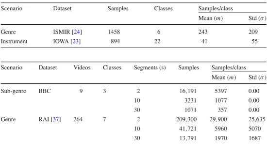
Table 1 Overview of the

employed audio datasets Scenario Dataset Samples Classes Samples/class

Mean (m) Std (σ)

Genre ISMIR [24] 1458 6 243 209

Instrument IOWA [23] 894 22 41 55

Table 2 Overview of the

employed video datasets Scenario Dataset Videos Classes Segments (s) Samples Samples/class Mean (m) Std (σ) Sub-genre BBC 9 3 2 16,191 5397 0.00 10 3231 1077 0.00 30 1071 357 0.00 Genre RAI [37] 264 7 2 209,300 29,900 25,635 10 41,721 5960 5070 30 13,791 1970 1687

Finally, it has to be stated that the proposed approach does not explicitly handle noisy features, which in general exhibit low correlations. For such a case, a preprocessing step (data cleaning) is needed to eliminate potentially noisy features. Such a step is not considered in this work.

4 Evaluation setup

4.1 Application scenarios and datasets

We investigate two audio classification scenarios: music

genreandinstrumentclassification. The two underlying real-world datasets demonstrate different degrees of difficulty in the context of high-dimensional data mining: strongly vary-ing number of samples in comparison with the overall feature dimensionality, number of classes, and class distribution (see Table1). Additionally, the nature of the data does not allow for any assumptions about the distribution of single feature components or complete group features. The datasets are well established in the domain of audio analysis and, thus, suitable for a comparison with related work.

Additionally, we investigate two video datasets: BBC documentaries and RAI TV broadcasts (see Table2). The BBC data is a self-collected set of 9 h of videos from the BBC’s YouTube channel.1 It covers three sub-genres:

technical,nature, andmusic. Although the semantic focus of the three sub-genres is strongly varying, all videos in this set are composed, edited, and post-processed in a very similar way, at least from a technical (editorial) point of view. The second video dataset contains more than 100 h of complete broadcasted programmes of RAI television and compromises 7 genres:commercials,football,music,news, 1_{https://www.youtube.com/user/BBC/.}

talk shows,weather forecasts, andcartoons[37,38]. In con-trast to the BBC documentaries, the RAI broadcasts exhibit strongly varying structures and no explicit regularities among the different genres. As a result, this heterogeneous cor-pus corresponds to a conventional genre classification task, whereas the BBC documentaries allow for the investigation of a sub-genre classification scenario. Since the different video datasets are available as different video container files, we first extract the audio tracks and convert them to PCM audio files. The audio tracks are segmented into chunks of 2, 10, and 30 s. This subdivision is carried out with an overlap of 50% in order to maintain acoustic information near the segmentation boundaries. Especially when con-sidering small segments of the audio signals, passages of constant silence may appear. These segments do not have any expressiveness and may cause errors in the feature extraction process. Therefore, we perform silence detec-tion by means of a noise threshold of−60 dB and remove detected silent segments from the dataset. This step has a low impact on the following analysis: none of the segments from the BBC documentaries and only 0.2% of the 2 s seg-ments from the RAI TV dataset are identified as silence and removed.

4.2 Audio features

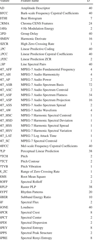
We employ a set of 50 group features (679 feature compo-nents in total) that includes representative and comprehensive audio features from the temporal and frequency domains. They represent different audio aspects, such as harmonic structure, rhythm, pitch, and loudness. For more details on all features please refer to [36]. Table3 provides an overview of the extracted features and the corresponding number of components (feature dimension).

Table 3 Overview of the employed features (in alphabetical order) and the corresponding dimensions (D)

Feature Feature name D

AD Amplitude Descriptor 40

BFCC Bark-scale Frequency Cepstral Coefficients 40

BTHI Beat Histogram 7

CRMA Chroma CENS Features 24

E4Hz 4 Hz Modulation Energy 2

GPD Group Delay 40

HMDV Harmonic Derivate 16

HZCR High Zero Crossing Rate 1

LPC Linear Predictive Coding 40

LPCC Linear Prediction Cepstral Coefficients 40

LPZC Linear Prediction ZCR 2

LSP Line Spectral Pairs 40

M7_AFF MPEG-7 Audio Fundamental Frequency 4

M7_AH MPEG-7 Audio Harmonicity 4

M7_AP MPEG-7 Audio Power 2

M7_ASB MPEG-7 Audio Spectrum Basis 72

M7_ASC MPEG-7 Audio Spectrum Centroid 2 M7_ASF MPEG-7 Audio Spectrum Flatness 34 M7_ASP MPEG-7 Audio Spectrum Projection 16

M7_ASS MPEG-7 Audio Spectrum Spread 2

M7_AW MPEG-7 Audio Waveform 4

M7_HSC MPEG-7 Harmonic Spectral Centroid 1 M7_HSD MPEG-7 Harmonic Spectral Deviation 1 M7_HSS MPEG-7 Harmonic Spectral Spread 1 M7_HSV MPEG-7 Harmonic Spectral Variation 1

M7_LAT MPEG-7 Log Attack Time 1

M7_SC MPEG-7 Spectral Centroid 1

MFCC Mel-scale Frequency Cepstral Coefficients 40

PLP Perceptual Linear Prediction 38

PTCH Pitch 2

PTCT Pitch Contour 2

PTVB Pitch Vibration 1

R_ZC Range of Zero Crossing Rate 1

RMS Root Mean Square 2

ROFF Spectral Rolloff 2

RPLP Raster PLP 38

RYPT Rhythm Patterns 20

SBER Subband Energy Ratio 10

SF Spectral Flux 2

SONE Loudness 40

SPCR Spectral Crest 8

SPCT Spectral Center 2

SPDI Spectral Dispersion 2

SPEY Spectral Entropy 8

SPPS Spectral Peak Structure 2

SPRE Spectral Renyi Entropy 8

Table 3 continued

Feature Feature name D

SPSL Spectral Slope 8

STE Short Time Energy 2

VDR Volume Dynamic Range 1

ZCR Zero Crossing Rate 2

679

4.3 Performance metrics

We consider two performance metrics: weighted F-score

for measuring the classification accuracy androbustnessfor measuring the reliability of a feature selection method to repeatedly select the same feature set for a given application scenario in different runs.

Theweighted F-scoreaccounts for the class distribution of the underlying dataset by building the arithmetic mean of the standardF-score values for the individual classes:

F_βw= 1 n

c_∈C

F_β(c)×nc, (2)

wherencdenotes the number of instances per classc,nis the

number of instances in total, andFβ is the standardF-score:

F_β =(1+β2) pr eci si on×r ecall

β2_{×pr eci si on+r ecall}. (3)

Up to now robustness (stability) has not been considered to be an issue in the domain of media analysis and media mining. This paper is one of the first to draw the attention to the fact that in dynamic environments and continuously changing large media repositories, robustness should be an important aspect of feature selection. Robust feature selec-tion has been addressed in other domains, such as in internet traffic anomaly detection [41] and, especially, in bioinformat-ics. Several approaches have been suggested for the analysis of gene expression data obtained from microarray experi-ments [1,4], for example in [19,39,44,58]. This challenging problem deals with a feature space of at least tens of thou-sands of genes, a small sample size, and noise and variability due to the experimental setup making the robustness of selected features an important goal.

Robustness measures are usually based on the similarity of feature sets. An approach producing very similar feature sets in different runs or in different tasks is considered to be robust. A very popular measure for set similarity in statistics is the Jaccard index defined as the cardinality of the intersec-tion divided by the cardinality of the union of two (or more) sets [31]. Additional measures have been introduced in the literature, and an overview and comparison is provided by

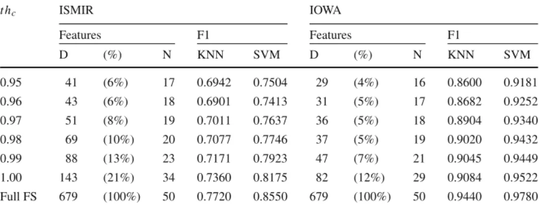
Table 4 Influence of the correlation threshold (t hc) on

the classification accuracy in terms of F1-scores (F1), number (N) of selected features, and dimensionality (D) of the corresponding feature subset in comparison to the full feature set (Full FS) for the employed audio datasets t hc ISMIR IOWA Features F1 Features F1 D (%) N KNN SVM D (%) N KNN SVM 0.95 41 (6%) 17 0.6942 0.7504 29 (4%) 16 0.8600 0.9181 0.96 43 (6%) 18 0.6901 0.7413 31 (5%) 17 0.8682 0.9252 0.97 51 (8%) 19 0.7011 0.7637 36 (5%) 18 0.8904 0.9340 0.98 69 (10%) 20 0.7077 0.7746 37 (5%) 19 0.9020 0.9432 0.99 88 (13%) 23 0.7171 0.7923 47 (7%) 21 0.9045 0.9449 1.00 143 (21%) 34 0.7360 0.8175 82 (12%) 29 0.9084 0.9522 Full FS 679 (100%) 50 0.7720 0.8550 679 (100%) 50 0.9440 0.9780 Somol and Novovicova [53]. We principally follow the

def-inition of the Jaccard index. However, we aim at making differences between approaches larger and more expressive by not using the cardinality of the union but the cardinality of the smaller set as divisor. We therefore measure robust-ness, R, of a feature selection approach by considering the co-occurrences of the selected features in a final feature set,

f S, averaged over a predefined number of independent and randomly initialized runs,r, as follows:

R= 2 r(r−1) r−1 i=1 r j=i+1 |f Si∩ f Sj| mi n(|f Si|,|f Sj|) (4) 4.4 Classifiers

We compare the performance of two well-established clas-sifiers for audio classification [14]: K-nearest neighbor (KNN) [6], and support vector machine (SVM) [56]. In pre-vious work, we additionally considered multinomial logistic regression (MLG) and random forest (RF) [5] in various audio-based scenarios [46]. Both MLG and RF classifiers demonstrated comparable performance to KNN and SVM at notably higher computational costs. Therefore, in this work we focus on the performance of KNN and SVM only. The classifier parameters have been selected based on prelimi-nary experiments on all investigated datasets with respect to classification accuracy and runtime performance. We employ KNN withk=1 and the Euclidean distance with no distance weighting. The SVM uses a linear kernel function. All clas-sifications are randomly initialized, 10-fold cross-validated with respect to the underlying class distribution, and run 10 times independently.

5 Evaluation results

5.1 Correlation threshold

In our first experiment, we elaborate the influence of the correlation threshold,t hc, on the selected feature set (both in

terms of dimensionality and number of selected features) and the resulting classification performance in terms ofF1-score. Additionally, we put the results in relation to the performance of the full feature set. For this experiment, we perform feature selection on 10% of the corresponding data in 10 randomly initialized runs. For the classification, each run is 10-fold cross-validated. Tables 4 and 5 summarize the achieved results averaged over the 10 independent runs for differ-ent correlation thresholds, t hc = {0.95,0.96, . . . ,1.00},

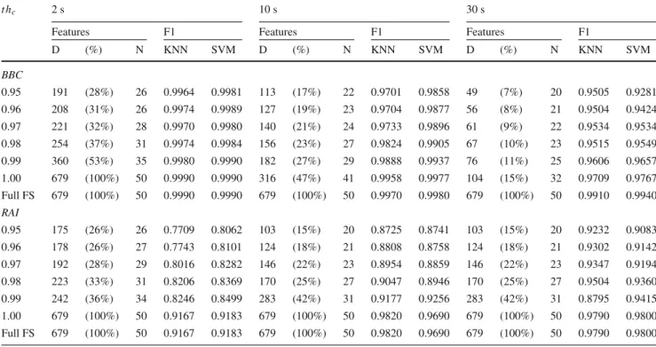
for the audio and video sets, respectively. The results show that an increase in the correlation threshold leads to an increase in both the dimensions of the selected feature set and the classification accuracy. This monotonic increase can be observed independently of the underlying classifier and dataset. Noteworthy is the remarkable reduction in feature dimensionality at a comparable performance level. For exam-ple, the BBC data with video segments of 2 s achieves an F1-score of 99.90% using the SVM classifier. The employ-ment of the proposed feature selection approach with a correlation threshold of 0.95 achieves a notable reduction in the feature set to 28% of the full feature set at highly com-parable classification performance indicated by the F1-score of 99.81%. The reduction in feature dimensionality leads to lower computational costs. Moreover, a lower feature set dimensionality supports the application of methods which cannot handle high-dimensional data.

The results additionally show a notable difference between the performance across the different segment sizes for the two video datasets. BBC performs better for smaller segments (e.g., F1-score of 99.81% for audio segments of size 2 s and F1-score of 92.81% for segments of size 30 s using the SVM classifier andt hc = 0.95). On the opposite side, the

RAI dataset performs slightly better for increasing segment sizes (e.g., F1-score of 80.62% for segments of size 2 s.2and F1-score of 90.83% for segments of size 30 s, again using the SVM classifier andt hc =0.95). This inverse tendency is

2 _{Please note that due to computational reasons we performed} clas-sification on 25% of the RAI dataset with segments of size 2 s as an approximation for the overall performance.

Table 5 Influence of the correlation threshold (t hc) on the classification accuracy in terms of F1-scores (F1), number (N) of selected features, and

dimensionality (D) of the corresponding feature subset in comparison to the full feature set (Full FS) for the employed video datasets

t hc 2 s 10 s 30 s

Features F1 Features F1 Features F1

D (%) N KNN SVM D (%) N KNN SVM D (%) N KNN SVM BBC 0.95 191 (28%) 26 0.9964 0.9981 113 (17%) 22 0.9701 0.9858 49 (7%) 20 0.9505 0.9281 0.96 208 (31%) 26 0.9974 0.9989 127 (19%) 23 0.9704 0.9877 56 (8%) 21 0.9504 0.9424 0.97 221 (32%) 28 0.9970 0.9980 140 (21%) 24 0.9733 0.9896 61 (9%) 22 0.9534 0.9534 0.98 254 (37%) 31 0.9974 0.9984 156 (23%) 27 0.9824 0.9905 67 (10%) 23 0.9515 0.9549 0.99 360 (53%) 35 0.9980 0.9990 182 (27%) 29 0.9888 0.9937 76 (11%) 25 0.9606 0.9657 1.00 679 (100%) 50 0.9990 0.9990 316 (47%) 41 0.9958 0.9977 104 (15%) 32 0.9709 0.9767 Full FS 679 (100%) 50 0.9990 0.9990 679 (100%) 50 0.9970 0.9980 679 (100%) 50 0.9910 0.9940 RAI 0.95 175 (26%) 26 0.7709 0.8062 103 (15%) 20 0.8725 0.8741 103 (15%) 20 0.9232 0.9083 0.96 178 (26%) 27 0.7743 0.8101 124 (18%) 21 0.8808 0.8758 124 (18%) 21 0.9302 0.9142 0.97 192 (28%) 29 0.8016 0.8282 146 (22%) 23 0.8954 0.8859 146 (22%) 23 0.9347 0.9194 0.98 223 (33%) 31 0.8206 0.8369 170 (25%) 27 0.9047 0.8946 170 (25%) 27 0.9504 0.9360 0.99 242 (36%) 34 0.8246 0.8499 283 (42%) 31 0.9177 0.9256 283 (42%) 31 0.8795 0.9415 1.00 679 (100%) 50 0.9167 0.9183 679 (100%) 50 0.9820 0.9690 679 (100%) 50 0.9790 0.9800 Full FS 679 (100%) 50 0.9167 0.9183 679 (100%) 50 0.9820 0.9690 679 (100%) 50 0.9790 0.9800

primarily due to the substantial difference in the nature of the underlying data. While the BBC data are very homogeneous (all documentaries share common structure and elements), the RAI data are distinctive to a certain degree. As a result, the BBC set requires higher granulated segments to capture more descriptive information and, thus, better distinguish across the different sub-genres of documentaries.

The comparison of the two classifiers, KNN and SVM, indicates existing data dependency of the overall perfor-mance in terms of F1-score. While for the audio datasets SVM notably outperforms KNN, for the video datasets the performance difference vanishes. In general, SVM outper-forms KNN. However, in very specific data settings (cp. RAI dataset, segment size of 30 s,t hc= {0.95,0.96,0.97,0.98})

KNN demonstrates superior performance over SVM at sig-nificantly lower computation costs.

Finally, we investigate the robustness of the proposed fea-ture selection approach, i.e., its ability to select the same features in different runs for the same dataset. Figure1shows the achieved results for all datasets for the previously con-sidered threshold settings. The results indicate two trends.

First, the larger the available data, the more robust is the selected feature set. For example, the RAI dataset with seg-ments of 2 s (209.300 samples in total) achieves an average intersection of 98.46% in contrast to the same dataset with segments of 30 s (13.791 samples in total) which achieves an average intersection of 85.57% fort hc=0.95. This

ten-dency can be observed over the different threshold settings

and for the three variations of the BBC dataset as well. Sec-ond, the higher the correlation threshold, the more robust the selected feature set. For example, the ISMIR dataset achieves 80.65% feature overlapping fort hc =0.95 and 97.37% for t hc = 1.00. This tendency is closely related to the number

of selected features and, again, independent of the underly-ing dataset. Overall, the average intersection over all datasets and threshold settings is 92% indicating the high robustness of the proposed feature selection approach.

5.2 Data size for feature selection

In this experiment, we investigate the influence of the size of available data on the feature selection process (in terms of dimensionality and number of the selected features and the robustness of the resulting feature sets over different runs on the same data) and on the classification performance (in terms of F1-scores). For this evaluation, we consider the two audio datasets, ISMIR and IOWA, and two video datasets, BBC and RAI, segments of size 30 s. We fix the correlation threshold, t hc, to 0.99 and consider different portion sizes

of the investigated datasets for the feature selection process (1, 5, 10, 20, 50, and 100%) in 10 randomly initialized and 10-fold cross-validated runs. The smallest class in the IOWA dataset is of size 9; therefore, the lowest reported portion for this dataset is 10%.

Table6summarizes the results in terms of dimensionality of the selected feature sets and the corresponding

classi-Correlation threshold (thc) 0.95 0.96 0.97 0.98 0.99 1.00 O v erlapping 0 0.2 0.4 0.6 0.8 1

ISMIR IOWA BBC - 2 sec. BBC - 10 sec. BBC - 30 sec. RAI - 2 sec. RAI - 10 sec. RAI - 30 sec.

Fig. 1 Overlapping of the selected features over the 10 independent and randomly initialized runs for the different datasets and threshold settings Table 6 Influence of the size of

the data available for feature selection on the classification accuracy in terms of F1-scores (F1), number (N) of selected features, and dimensionality (D) of the corresponding feature subset in comparison to the full feature set (Full FS) for the investigated datasets

Audio datasets

Data ISMIR IOWA

Features F1 Features F1 D (%) N KNN SVM D (%) N KNN SVM 1% 11 (2%) 9 0.5986 0.6057 – – – – – 5% 45 (7%) 20 0.7007 0.7727 – – – – – 10% 88 (13%) 23 0.7171 0.7923 47 (7%) 21 0.9045 0.9449 20% 135 (20%) 26 0.7250 0.8029 97 (14%) 24 0.8971 0.9506 50% 199 (29%) 29 0.7453 0.8255 234 (34%) 25 0.8757 0.9415 100% 225 (33%) 32 0.7560 0.8310 276 (41%) 29 0.8990 0.9520 Full FS 679 (100%) 50 0.7720 0.8550 679 (100%) 50 0.9440 0.9780 Video datasets Data BBC-30 s RAI-30 s Features F1 Features F1 D (%) N KNN SVM D (%) N KNN SVM 1% 8 (1%) 7 0.8281 0.6567 80 (12%) 23 0.9276 0.9090 5% 42 (6%) 25 0.9637 0.9314 240 (35%) 30 0.9094 0.9420 10% 76 (11%) 25 0.9606 0.9657 283 (42%) 31 0.8795 0.9415 20% 145 (21%) 27 0.9701 0.9802 328 (48%) 32 0.9089 0.9562 50% 301 (44%) 31 0.9690 0.9930 320 (47%) 35 0.9122 0.9575 100% 357 (53%) 33 0.9810 0.9930 340 (50%) 33 0.9120 0.9580 Full FS 679 (100%) 50 0.9910 0.9940 679 (100%) 50 0.9790 0.9800 fication performance. The results show that an increasing

size of available data for feature selection usually leads to a higher number of selected features. This is due to the fact that more data usually reveals more aspects about the underlying data characteristics. Therefore, a larger number of features is required to capture more descriptive information. However, while the amount of data for the feature selection is rapidly growing, the size of the selected feature set only displays a slight increase. This indicates that, at some point no addi-tional information is introduced by newly added instances. Overall, the size of the selected feature set is again notably lower than the size of the full feature set.

Figure2shows the robustness of the selected feature sets over the different runs for each of the investigated datasets. The results reflect the previous observations. The random selection of a low portion of data (e.g., 1–5%) may poten-tially lead to the selection of data subsets that capture very differing characteristics resulting in a (relatively) low inter-section of the selected feature sets. In contrast, the probability that a larger data subset will account for a greater deal of the characteristics of the underlying data is significantly higher. Therefore, the more data are available for the feature selec-tion process, the higher the robustness of the selected feature set. Nevertheless, the results show that performing feature

% Data 1% 5% 10% 20% 50% 100% O v erlapping 0 0.2 0.4 0.6 0.8 1

ISMIR IOWA BBC - 30 sec. RAI - 30 sec.

Fig. 2 Overlapping of the selected features over the 10 independent and randomly initialized runs for varying percentages of available data for feature selection for the investigated datasets

selection on 10% of the data already achieves highly robust feature sets with an intersection of approx. 90% over the dif-ferent randomly initialized runs.

5.3 Comparison to related work on feature selection

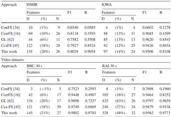
In this section, we compare the performance of the pro-posed group feature selection approach with our previous work, CcaFS [45], which applies CCA on feature pairs, with two well-established but supervised subset-based feature selection approaches, consistency-based (ConFS) [34] and correlation-based(CorrFS) [16], and with the group feature selection approach group lasso (GL) [62]. For all approaches, we perform feature selection and model building for the clas-sifier on 20% of the available data. The performance on the remaining data is evaluated in terms of both F1-score and robustness of the selected feature sets averaged over 10 inde-pendent and randomly initialized runs. For the classification, we employ the SVM classifier and perform 10-fold cross-validation of each run.

Table7condenses the results for the four data sets, ISMIR, IOWA, BBC (30 s) and RAI (30 s), in terms of the selected feature set dimension (D), the percentage of compression in comparison to the initial (full) feature set (%), F1-score using the SVM classifier, and robustness (R). The results show no overall winner over all four datasets in terms of F1-score: Group lasso achieves the best F1-score for BBC and RAI, and the supervised correlation-based approach the best results for ISMIR and IOWA. Our approach is second for three datasets and third for IOWA, however, with very small differences to the best approaches. Robustness shows an entirely different picture: Our approach is best in three cases, but usually with large differences to the other methods. The number of fea-tures selected is largest for our first approach CcaFS in three cases. A comparison of our new and our first approaches shows that we could improve F1-scores and robustness and at the same time reduce the number of selected features. Only in the case of the IOWA dataset, robustness could not be

improved. Overall, we demonstrated that our new, unsuper-vised approach yields comparable results in terms of F1-score to the other approaches while at the same time yielding con-siderably better robustness.

5.4 Comparison to related work on media classification

In this section, we present a comparison of the results achieved by the proposed approach with related works report-ing results on the same three publicly available datasets: ISMIR (music genre classification), IOWA (musical instru-ment identification), and RAI (TV genre classification).

For the first ISMIR music dataset, we rerun the experi-ments with the same settings as defined by the ISMIR 2004 genre classification contest3 in order to provide for com-parability. In the contest, the classification performance is evaluated based on predefined training and test sets (con-sisting of 729 samples each) using weighted classification accuracy:

C A=

c∈genr es

pcC Ac; (5)

where pc is the probability of appearance of genre c and C Ac the classification accuracy for c. Table8 provides a

summary of most recent works reporting top results on the ISMIR dataset. In general, research in the context of music genre classification is highly tailored to the characteristics of the specific task. For example, Lee et al. [30] elaborate long-term modulation spectral analysis of spectral and cesp-tral feature trajectories to describe the time-varying behavior of music signals. The authors investigate octave-based spec-tral contrast (OSC), normalized audio spectrum envelope (NASE), and MFCC features. Overall, the listed approaches exhibit a broad variety in the dimensionality of the considered feature sets. For example, Seo and Lee [48] employ higher-3 _{http://ismir2004.ismir.net/genre_contest.}

Table 7 Comparison to related feature selection algorithms in terms of number (N) of selected features and their dimensionality (D), F1-scores using the SVM classifier, and robustness (R) of the corresponding feature selection approach

Audio datasets

Approach ISMIR IOWA

Features F1 R Features F1 R D (%) N D (%) N ConFS [34] 10 (1%) 9 0.6540 0.0585 4 (1%) 4 0.6602 0.1278 CorrFS [16] 69 (10%) 26 0.8118 0.3593 88 (13%) 31 0.9685 0.4399 GL [62] 44 (6%) 11 0.7582 0.5508 85 (13%) 13 0.9620 0.8545 CcaFS [45] 122 (18%) 28 0.7927 0.8524 82 (12%) 25 0.9426 0.8654 This work 135 (20%) 26 0.8029 0.9054 97 (14%) 24 0.9506 0.8108 Video datasets Approach BBC-30 s RAI-30 s Features F1 R Features F1 R D (%) N D (%) N ConFS [34] 3 (<1%) 3 0.7523 0.2593 8 (1%) 7 0.7698 0.1960 CorrFS [16] 42 (6%) 17 0.9448 0.4907 105 (16%) 27 0.9464 0.8252 GL [62] 134 (20%) 17 0.9898 0.7237 425 (63%) 26 0.9797 0.9659 Cca-FS [45] 121 (18%) 30 0.9749 0.8869 248 (37%) 34 0.9479 0.9138 This work 145 (21%) 27 0.9802 0.9703 328 (48%) 32 0.9562 0.9771

order moments of short-time spectral features building a 72-dimensional feature vector and achieving a classification accuracy of 84.64%. On the opposite side, Seyerlehner et al. [49] employ block-based features of dimensionality 9448 leading to a classification accuracy of 88.27%. Although, our approach is outperformed by approximately 10% by Lee et al. [30], it is the only approach that autonomously selects features to represent the provided data. In contrast, Baniya et al. [2], for example, manually omit features based on the standard deviation of the considered features in the very spe-cific data settings. Overall, the lower result by our approach is probably caused by the initial set of 50 features which con-sists of fundamental and representative audio features only, describing a broad range of general audio characteristics. This implies that we are not employing any task-specific analysis or classification as in the work by Lee et al. [30], for example.

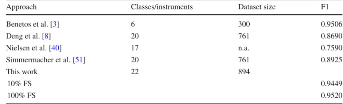
Table9summarizes reported results of related approaches on the IOWA dataset. A direct comparison of the results and the underlying approaches is not possible given the major dif-ferences in the employed data and the experimental settings. For example, Benetos et al. [3] report top performance on the IOWA dataset in terms of F1-score of 95.06%. However, the authors employ only a small subset of the available data con-sisting of a well-defined selection of 6 instruments: piano, bassoon, cello, flute, sax, and violin. In contrast, the works by Deng et al. [8] and Simmermacher et al. [51] employ nearly the same dataset size and only omit two instruments: guitar and marimba. Still, the authors simplify the

experi-Table 8 Comparison to related works on the ISMIR dataset (in alpha-betical order) in terms of considered feature dimensionality (D) and the resulting weighted classification accuracy (CA)

Approach Classifier D CA

Baniya et al. [2] ELM [21] 144 0.8646

Jang and Jang [25] SVM 168 0.8340

Lee et al. [30] LDA [10] n.a. 0.8683

Lim et al. [32] SVM 468 0.8990

Seyerlehner et al. [49] SVM 9448 0.8827

Seo and Lee [48] SVM 72 0.8464

This work SVM 334 0.7792

mental settings and employ the same number of samples for the instruments within each category. In our experiments, we keep the original distribution of samples which provides for a notably imbalanced data setting. Table 10shows the confusion matrix of the individual instrument classification using 10-fold cross-validation; feature selection is performed using the full dataset witht hc =0.99. In general, our results

confirm the findings by Deng et al. [8] and Simmermacher et al. [51]. The best classification accuracies are achieved by the

piano/othersandpercussioncategories with 100%, followed by thestringinstruments with 99%. Worst average classifi-cations accuracy is achieved within thewoodwindcategory by samples ofbass flute classified asalto flute(and partly vice versa). In contrast to Deng et al. [8] and Simmermacher et al. [51], we identify thebrasscategory as the one with the lowest average classification accuracy of 78%. Overall, our

Table 9 Comparison to related works (in alphabetical order) on the IOWA dataset with respect to the considered

classes/instruments and the resulting classification accuracy in terms of F1-scores (F1)

Approach Classes/instruments Dataset size F1

Benetos et al. [3] 6 300 0.9506

Deng et al. [8] 20 761 0.8690

Nielsen et al. [40] 17 n.a. 0.7590

Simmermacher et al. [51] 20 761 0.8925

This work 22 894

10% FS 0.9449

100% FS 0.9520

FS denotes the percentage of data employed for the feature selection witht hc=0.99 Table 10 IOWA confusion matrix of 10-fold cross-validation (in percentage)

Instrument # _{a b c d e f g h i j}Classified as_{k l m n o p q r s t u v} Piano/others: a=Piano 260 100 b=Guitar 45 100 Brass: c=Tuba 9 100 d=BbTrumpet 24 96 4 e=Horn 12 67 8 25 f=TenorTrombone 12 58 25 17 g=BassTrombone 12 58 25 17 String: h=Violin 71 100 i=Viola 62 100 j=DoubleBass 71 100 k=Cello 79 3 96 1 Woodwind: l=BbSopranoSax 25 92 4 4 m=AltoSax 18 100 n=Oboe 12 17 8 8 67 o=Bassoon 15 13 87 p=Flute 22 100 q=AltoFlute 11 82 18 r=BassFlute 10 10 50 40 s=BassClarinet 12 83 17 t=BbClarinet 14 7 7 7 79 u=EbClarinet 14 7 7 86 Percussion: v=marimba 84 100

Per instrument category 100 78 99 85 100

Feature selection (FS) is performed using the full dataset witht hc=0.99. # denotes the number of samples for each instrument. The last line shows

the weighted average classification rate per instrument category

proposed approach outperforms previous works in terms of F1-score of 95.20%.

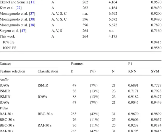
Eventually, we compare our approach with related works reporting evaluation results on the RAI dataset (see Table11).4 In contrast to the previous audio sets, the RAI video dataset allows for the development and comparison of approaches using different modalities. Recent works demonstrate a ten-dency toward multimodal approaches [11,37,38]. The results achieved by our approach indicate the outstanding perfor-mance of the selected audio features in terms of F1-score of 95.80% despite the use of single modality only. Addition-ally, our approach demonstrates strong competitiveness to the top reported performance by Ekenel and Semela [11]. In addition to some acoustic features, Ekenel and Semena consider visual, structural, and cognitive features. Similar to the works by Montagnuolo et al. [37,38], the features are selected in a way which reflects the editors process in TV production and cannot be applied to arbitrary data. The audio-based approach by Ekenel and Semela [11] achieves comparable performance in terms of F1-score of 95.70%. 4_{Please note that the information on the number of videos and their} duration in the table may partially differ from the information in the referenced works due to corrected rounding or computation errors.

However, the approach is supervised and relies on available data in order to train a SVM model for each genre separately using manually selected features. In contrast, our approach autonomously selects the features that are relevant for the provided dataset and it is not bound to a specific applica-tion or dataset. The achieved performance demonstrates the quality of the selected features while at the same time the exploration of a single modality notably reduces the compu-tational effort.

5.5 Data sensitivity

Feature selection is commonly done in a very specific con-text: for a particular application scenario or even for a specific data setting. An initial investigation of the selected fea-ture sets for the considered datasets revealed a high degree of overlapping, i.e., 81% between the selected features for the audio datasets ISMIR and IOWA and even 90% for the video datasets BBC and RAI (30 s segments). This is noteworthy since the datasets target different application scenarios. One might argue that the remaining 10 or 19% would be crucial for the classification performance in the corresponding settings. The alternative hypothesis is that a

Table 11 Comparison to related works (in alphabetical order) on the RAI dataset in terms of considered modalities: audio (A), visual (V), structural (S), cognitive(C), and the resulting classification accuracy in terms of F1-scores (F1)

Approach Modality Videos Duration (in min) F1

Ekenel and Semela [11] A, V, S, C 262 4,164 0.9920

Ekenel and Semela [11] A 262 4,164 0.9570

Kim et al. [27] A 262 4,164 0.9430

Montagnuolo et al. [37] A, V, S, C n.a. 6,692 0.9200

Montagnuolo et al. [38] A, V, S, C 396 6,672 0.9490

Montagnuolo et al. [38] A 396 6,672 0.7870

Sargent et al. [47] A, V, S 264 n.a. 0.7160

This work A 264 4,175

10% FS 0.9415

100% FS 0.9580

Table 12 Evaluation of the classification performance of feature selection on a related dataset

Dataset Features F1

Feature selection Classification D (%) N KNN SVM

Audio IOWA ISMIR 47 (7%) 21 0.6891 0.7727 ISMIR 88 (13%) 23 0.7171 0.7923 ISMIR IOWA 88 (13%) 23 0.9182 0.9477 IOWA 47 (7%) 21 0.9045 0.9449 Video RAI-30 s BBC-30 s 283 (42%) 31 0.9670 0.9899 BBC-30 s 76 (11%) 25 0.9606 0.9657 BBC-30 s RAI-30 s 76 (11%) 25 0.9238 0.9184 RAI-30 s 283 (42%) 31 0.8795 0.9415

Feature selection is performed on 10% of the corresponding data witht hc=0.99

well-defined feature set is competitive for a broad range of data and application settings. Therefore, in the following experiments we investigate the interrelation between data (and thus the underlying application scenario) and selected feature set, and its influence on the classification perfor-mance in more detail. Again, all experiments are based on 10 independent and randomly initialized runs and 10-fold cross-validated.

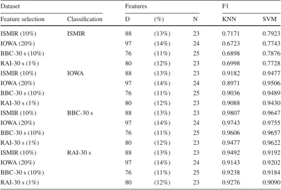
In our first experiment, we exchange the selected fea-ture sets for the two audio datasets, ISMIR and IOWA, and for two video datasets, BBC and RAI (30 s segments), i.e., we employ features selected on the one dataset (e.g., ISMIR) to perform media classification on the second dataset related in terms of employed media (e.g., IOWA). Table12 compares the achieved results in terms of F1-scores to the results using the original feature set, i.e., the features selected using the very same dataset as for the classification. The potentially expected drop in the classification scores cannot be confirmed. In fact, overall, the switch of the underly-ing feature sets leads to comparable performances for all datasets. The slight variations in the F1-scores indicate a dependency on the size of the feature set rather than on

the dataset originally employed for the feature selection pro-cess. Therefore, we repeat the experiment with a comparable size of the selected feature set (in terms of resulting dimen-sionality). Additionally, we perform cross-media exchange of the selected feature sets to magnify potential depen-dencies between selected features and underlying data and application scenarios. Table 13 summarizes the achieved results. Again, the classification performance for a single dataset shows only slight deviations although the feature selection has been performed on partly strongly varying data and for a different application scenario. For exam-ple, the SVM classifier achieves an F1-score of 79.23% for the ISMIR audio data using features selected on the very same data in contrast to an F1-score of 78.76% using fea-tures selected on the dataset consisting of BBC documentary videos.

The results seem to support the assumption, that a well-defined feature set can be employed for a broad range of application scenarios. The question arises how to addition-ally increase the applicability of the selected feature set for varying data and application scenarios. We consider two possibilities. The first scenario accounts for the situation

Table 13 Evaluation of the classification performance of feature selection on a different dataset

Dataset Features F1

Feature selection Classification D (%) N KNN SVM

ISMIR (10%) ISMIR 88 (13%) 23 0.7171 0.7923 IOWA (20%) 97 (14%) 24 0.6723 0.7743 BBC-30 s (10%) 76 (11%) 25 0.6898 0.7876 RAI-30 s (1%) 80 (12%) 23 0.6998 0.7728 ISMIR (10%) IOWA 88 (13%) 23 0.9182 0.9477 IOWA (20%) 97 (14%) 24 0.8971 0.9506 BBC-30 s (10%) 76 (11%) 25 0.9036 0.9489 RAI-30 s (1%) 80 (12%) 23 0.9088 0.9430 ISMIR (10%) BBC-30 s 88 (13%) 23 0.9807 0.9647 IOWA (20%) 97 (14%) 24 0.9743 0.9755 BBC-30 s (10%) 76 (11%) 25 0.9606 0.9657 RAI-30 s (1%) 80 (12%) 23 0.9477 0.9622 ISMIR (10%) RAI-30 s 88 (13%) 23 0.9492 0.9192 IOWA (20%) 97 (14%) 24 0.9143 0.9202 BBC-30 s (10%) 76 (11%) 25 0.9238 0.9184 RAI-30 s (1%) 80 (12%) 23 0.9276 0.9090

Feature selection is performed witht hc=0.99, numbers in brackets denote the portion of data for feature

selection

where only a single dataset is available. Our previous exper-iment demonstrated that the analysis of a small portion of the data already allows for the selection of a competitive feature set (see Sect. 5.2). This is an especially efficient approach when working with very large datasets. However, there is no guarantee that even a random selection will cover most data characteristics of the underlying set. Increasing the selected data size for feature selection can increase the probability for a high portion of the present data charac-teristics (cp. Sect.5.2). Nevertheless, the determination of the data size for feature selection is not a trivial task since it is strongly dependent on both the available data and on the specific data characteristics. Another approach to cover for broader data characteristics than in a single data portion is repeating the feature selection process and unifying the selected features. For this purpose in each run (out of ten), we perform feature selection for randomly selected data por-tions and merge the extracted features into anunified feature set. In order to provide for comparability of the results, we keep the corresponding data portion sizes as in our previ-ous experiment: IOWA 20%, ISMIR 10%, BBC 10%, and RAI 1% (cp. Table13). The second scenarioaccounts for the situation where multiple datasets are available. In this case, we merge the unified feature sets for all datasets into a singleunified feature set (all data). Table14summarizes the achieved results and compares them to the performance of the original feature set (the result of a single data portion) and to the performance of the full feature set. Overall, the con-sideration of different portions of the data,unified feature

set, improves the expressiveness of the selected features and leads to an increase in the classification performance in terms of F1-score in comparison to the original feature set. The employment of further datasets,unified feature set (all data), additionally improves the expressiveness of the selected fea-ture set. Noteworthy is the fact that although this feafea-ture set has been selected in an unsupervised manner, it facili-tates partly strongly differing data and application scenarios. Furthermore, theunified feature set (all data)outperforms previously achieved results (cp. Table13) and it approaches the classification performance of the full feature set with sig-nificantly lower dimensionality (31%).5

The performed experiments confirm the fact that, in gen-eral, the employment of more features6will most probably increase the classification performance of a feature set since different features usually capture different data character-istics. Hence, the results achieved by the full feature set outperform the results of the selected feature sets for all considered datasets. However, the addition of any further feature inevitably leads to an increase in both the dimen-sionality of the resulting feature set and the computational costs while the overall performance might only improve

5 _{The finalunified feature set (all data)consists of the following 35} fea-tures (in alphabetical order): BTHI, CRMA, E4Hz, HMDV, HZZCR, LPZC, M7_AFF, M7_AH, M7_AP, M7_ASC, M7_ASF, M7_ASP, M7_ASS, M7_AW, M7_HSC, M7_HSD, M7_HSS, M7_HSV, M7_LAT, M7_SC, PTCH, PTCT, PTVB, ROFF, RPLP, RYPT, R_ZC, SF, SPCR, SPCT, SPDI, SPPS, STE, VDR, ZCR.

Table 14 Evaluation of the classification performance of the unified feature selection process for the different datasets

Dataset Feature set Features F1

D (%) N KNN SVM

ISMIR Original feature set 88 (13%) 23 0.7171 0.7923

Unified feature set 149 (22%) 31 0.7470 0.8170

Unified feature set (all data) 213 (31%) 35 0.7360 0.8340

Full feature set 679 (100%) 50 0.7720 0.8550

IOWA Original feature set 97 (14%) 24 0.8971 0.9506

Unified feature set 167 (25%) 30 0.9180 0.9600

Unified feature set (all data) 213 (31%) 35 0.9260 0.9660

Full feature set 679 (100%) 50 0.9440 0.9780

BBC-30 s Original feature set 76 (11%) 25 0.9606 0.9657

Unified feature set 115 (17%) 31 0.9790 0.9840

Unified feature set (all data) 213 (31%) 35 0.9890 0.9930

Full feature set 679 (100%) 50 0.9910 0.9940

RAI-30 s Original feature set 80 (12%) 23 0.9276 0.9090

Unified feature set 109 (16%) 29 0.9460 0.9240

Unified feature set (all data) 213 (31%) 35 0.9500 0.9480

Full feature set 679 (100%) 50 0.9790 0.9800

Feature selection is performed witht hc=0.99

marginally. Therefore, feature selection is commonly applied to reduce dimensionality and computational costs. The main drawback of existing approaches is that they are tailored to specific data and/or application scenario. Any alteration of the data settings or the underlying application scenario requires a reconsideration of the employed features. In con-trast, our last experiments demonstrate that the proposed unsupervised feature selection approach allows for the iden-tification of a highly expressive feature set that can be applied for different data and application scenarios even if the feature selection is performed on a small portion of the available data. This is a crucial benefit in a dynamic environment where data continuously changes and application scenarios are subject to adaptation.

6 Conclusion

In this paper, we presented an unsupervised approach for the selection of robust multi-dimensional (group) features that exploits canonical correlation in order to separate rele-vant from less relerele-vant features. In contrast to related works in the context of audio and video classification, the pro-posed approach preserves the original grouping of feature components into multi-dimensional (group) features, which results in a semantically interpretable feature selection. The approach is generic as it does not make any assumptions about the underlying data (or even application or task) char-acteristics, but it autonomously selects a feature set that efficiently describes the data. In addition, the feature set

selected by our approach is remarkably robust: different runs or even experiments for different tasks show little varia-tions in the set of selected features, even if the underlying training set varies considerably. We performed experiments on various audio and video datasets representing differ-ent application scenarios and data characteristics such as a strongly varying number of samples and classes and a varying class distribution. Achieved results show that our unsuper-vised approach is competitive to related works which were designed to solve very specific tasks and additionally demon-strates extraordinary robustness.

The reported experiments investigating the interrelation between selected features and provided data reveal some valuable insights. Achieved results indicate that the depen-dencies between data (and application scenario), and selected features are weaker than actually expected. The same well-selected features can discriminate both between viola and violin sounds and between different types of video documen-taries, for example. An approach which is highly tailored to a particular task will most probably additionally improve the performance in terms of classification accuracy and/or fea-ture dimensionality. However, any alteration of the task (such as the consideration of an additional label) will require the reconsideration of the employed features. In contrast, the per-formed experiments indicate that a single, highly expressive feature set can be applied for different data and application scenarios achieving highly competitive results. Such a robust data-driven approach is the only possibility when mining dynamic or unknown data collections where no prior infor-mation about the data is available. We believe that more

attention and research time should be paid in the future to the general question of how to obtain more robust features in such environments.

Acknowledgements Open access funding provided by TU Wien

(TUW). This work has been partly funded by the Vienna Science and Technology Fund (WWTF) through project ICT12-010. The authors would like to thank Maurizio Montagnuolo from RAI Centre for Research and Technological Innovation for providing the RAI TV dataset.

Open Access This article is distributed under the terms of the Creative Commons Attribution 4.0 International License (http://creativecomm ons.org/licenses/by/4.0/), which permits unrestricted use, distribution, and reproduction in any medium, provided you give appropriate credit to the original author(s) and the source, provide a link to the Creative Commons license, and indicate if changes were made.

References

1. Babu MM (2004) Introduction to microarray data analysis. Comput Genom Theory Appl 17(6):225–249

2. Baniya BK, Ghimire D, Lee J (2015) Automatic music genre clas-sification using timbral texture and rhythmic content features. In: International conference on advanced communication technology, pp 434–443

3. Benetos E, Kotti M, Kotropoulos C (2006) Musical instrument classification using non-negative matrix factorization algorithms and subset feature selection. In: IEEE international conference on acoustics, speech and signal processing, vol 5, pp 1844–1847 4. Berrar DP, Dubitzky W, Granzow M et al (2003) A practical

approach to microarray data analysis. Springer, New York 5. Breiman L (2001) Random forests. Mach Learn 45(1):5–32 6. Cover T, Hart P (1967) Nearest neighbor pattern classification.

IEEE Trans Inf Theory 13(1):21–27

7. Dash M, Liu H (1997) Feature selection for classification. Intell Data Anal 1:131–156

8. Deng J, Simmermacher C, Cranefield S (2008) A study on fea-ture analysis for musical instrument classification. IEEE Trans Syst Man Cybern B Cybern 38(2):429–438

9. Doraisamy S, Golzari S, Norowi NM, Sulaiman MN, Udzir NI (2008) A study on feature selection and classification techniques for automatic genre classification of traditional malay music. In: International conference on music information retrieval, pp 331– 336

10. Duda RO, Hart PE, Stork DG (2000) Pattern classification. Wiley-Interscience, New York, NY

11. Ekenel HK, Semela T (2013) Multimodal genre classification of TV programs and YouTube videos. Multimed Tools Appl 63(2):547– 567

12. Fiebrink R, Fujinaga I (2006) Feature selection pitfalls and music classification. In: International conference on music information retrieval

13. Friedman J, Hastie T, Tibshirani R (2010) A note on the group lasso and a sparse group lasso. ArXiv e-prints

14. Fu Z, Lu G, Ting KM, Zhang D (2011) A survey of audio-based music classification and annotation. IEEE Trans Multimedia 13(2):303–319

15. Guyon I, Elisseeff A (2003) An introduction to variable and feature selection. J Mach Learn Res 3:1157–1182

16. Hall MA (1999) Correlation-based feature subset selection for machine learning. Ph.D. thesis, University of Waikato

17. Hall MA, Holmes G (2003) Benchmarking attribute selection tech-niques for discrete class data mining. IEEE Trans Knowl Data Eng 15(6):1437–1447

18. Hall P, Miller H (2009) Using generalized correlation to effect variable selection in very high dimensional problems. J Comput Graph Stat 18(3):533–550

19. Hossain MZ, Kabir MM, Shahjahan M (2016) A robust feature selection system with Colin’s CCA network. Neurocomputing 173:855–863

20. Hotelling H (1936) Relations between two sets of variates. Biometrika 28(3/4):321–377

21. Huang GB, Zhu QY, Siew CK (2006) Extreme learning machine: theory and applications. Neurocomputing 70(1–3):489–501 22. Huang YF, Lin SM, Wu HY, Li YS (2014) Editorial: music genre

classification based on local feature selection using a self-adaptive harmony search algorithm. Data Knowl Eng 92:60–76

23. IOWA Dataset: Univ. of Iowa musical instrument samples.http:// theremin.music.uiowa.edu(1997)

24. ISMIR 2004 Dataset: International conference on music informa-tion retrieval—audio descripinforma-tion contest data set.http://ismir2004. ismir.net/(2004)

25. Jang D, Jang SJ (2014) Very short feature vector for music genre classification based on distance metric learning. In: International conference on audio, language and image processing, pp 726–729 26. Jang D, Jin M, Yoo CD (2008) Music genre classification using novel features and a weighted voting method. In: IEEE international conference on multimedia and expo, pp 1377–1380

27. Kim S, Georgiou P, Narayanan S (2013) On-line genre classifica-tion of TV programs using audio content. In: IEEE internaclassifica-tional conference on acoustics, speech and signal processing, pp 798–802 28. Kohavi R, John GH (1997) Wrappers for feature subset selection.

Artif Intell 97(1–2):273–324

29. Kononenko I (1994) Estimating attributes: analysis and extensions of RELIEF. In: European conference on machine learning, pp 171– 182

30. Lee CH, Shih JL, Yu KM, Lin HS (2009) Automatic music genre classification based on modulation spectral analysis of spectral and cepstral features. IEEE Trans Multimedia 11(4):670–682 31. Levandowsky M, Winter D (1971) Distance between sets. Nature

234(5323):34–35

32. Lim SC, Lee JS, Jang SJ, Lee SP, Kim MY (2012) Music-genre classification system based on spectro-temporal features and fea-ture selection. IEEE Trans Consum Electron 58(4):1262–1268 33. Liu H, Setiono R (1995) Chi2: feature selection and discretization

of numeric attributes. In: International conference on tools with artificial intelligence, pp 388–391

34. Liu H, Setiono R (1996) A probabilistic approach to fea-ture selection—a filter solution. In: International conference on machine learning, pp 319–327

35. Meier L, Geer SVD, Bühlmann P (2008) The group lasso for logis-tic regression. J R Stat Soc Series B Stat Methodol 70(1):53–71 36. Mitrovic D, Zeppelzauer M, Breiteneder C (2010) Features for

content-based audio retrieval. In: Advances in computers: improv-ing the web, vol 78, chap 3, pp 71–150. Elsevier

37. Montagnuolo M, Messina A (2007) TV genre classification using multimodal information and multilayer perceptrons. In: AI*IA 2007: artificial intelligence and human-oriented computing, pp 730–741

38. Montagnuolo M, Messina A (2009) Parallel neural networks for multimodal video genre classification. Multimed Tools Appl 41(1):125–159

39. Nie F, Huang H, Cai X, Ding CH (2010) Efficient and robust feature selection via joint2,1-norms minimization. In: International con-ference on neural information processing systems, pp 1813–1821 40. Nielsen AB, Sigurdsson S, Hansen LK, Arenas-Garcia J (2007) On the relevance of spectral features for instrument classification.