PAC-Bayesian High Dimensional Bipartite
Ranking
Benjamin Guedj*and Sylvain Robbiano†
May 20, 2019
Abstract
This paper is devoted to the bipartite ranking problem, a classical sta-tistical learning task, in a high dimensional setting. We propose a scoring and ranking strategy based on the PAC-Bayesian approach. We consider nonlinear additive scoring functions, and we derive non-asymptotic risk bounds under a sparsity assumption. In particular, or-acle inequalities in probability holding under a margin condition assess the performance of our procedure, and prove its minimax optimality. An MCMC-flavored algorithm is proposed to implement our method, along with its behavior on synthetic and real-life datasets.
Keywords:Bipartite Ranking, High Dimension and Sparsity, MCMC, PAC-Bayesian Aggregation, Supervised Statistical Learning.
1
Introduction
The bipartite ranking problem appears in various application domains such as medical diagnostic, information retrieval, signal detection. This super-vised learning task consists in building a so-called scoring function that or-der the (high dimensional) observations in the same fashion as the (unknown) associated labels. In that sense, the global problem of bipartite ranking (or-dering a set observations) includes the local classification task (assigning a label to each observation). Indeed, once a proper scoring function is defined, classification amounts to choosing a threshold, assigning data points to either class depending on whether their score is above or below that threshold. The quality of a scoring function is usually assessed through its ROC curve [Receiver Operating Characteristic, see20] and it is shown that maximizing this visual tool is equivalent to solving the bipartite ranking problem [see for example, Proposition 6 in13]. Due to the functional nature of the ROC curve, it is useful to substitute a proxy: maximizing the Area Under the ROC Curve (AUC), or equivalently minimizing the pairwise risk. Following that
*Modal project-team, Inria, France.[email protected]
†Department of Statistical Science, UCL, United Kingdom.[email protected]
idea, several classical algorithms in classification have been extended to the case of bipartite ranking, such as Rankboost [19] or RankSVM [30]. Several authors have considered theoretical aspects of this problem. In [1], the au-thors investigate the difference between the empirical AUC and the true AUC and produce a concentration inequality assessing that as the number of ob-servations increases, the empirical AUC tends to the true AUC, allowing for empirical risk minimization (ERM) approaches to tackle the bipartite rank-ing problem. This strategy has been explored by [14]. Assuming that the true scoring function is in a Vapnik-Cervonenkis class of finite dimension, combined with a low noise condition, the authors prove that the minimizer of the empirical pairwise risk achieves fast rates of convergence. More recently, the bipartite ranking problem has been tackled from a nonparametric angle and [12] proved that a plug-in estimator of the regression function can at-tain minimax fast rates of convergence over Hölder class. In order to obat-tain an adaptive estimator to the low noise and to the Hölder parameters, an ag-gregation procedure based on exponential weights has been proposed by [32] and the author shows adaptive fast rate upper bounds. However, the rates of convergence depend on the dimension of the features space and in many applications the optimal scoring function depends on a small number of the features, suggesting a sparsity assumption. As a matter of fact, the prob-lem of sparse bipartite ranking has been studied by [26]. The authors obtain general PAC results for the Gibbs estimator and deduce an oracle bound for linear scoring function under mild assumptions. In this paper, we consider the case of non-parametric scoring functions that can be sparsely decomposed in an additive way with respect to the covariates. Our results hold with hy-pothesis tailored for the ranking case and a specific set of candidate scoring function that allow for non-parametric rates.
To do so, we design an aggregation strategy which heavily relies on the PAC-Bayesian paradigm (the acronym PAC stands for Probably Approximately Correct). In our setting, the PAC-Bayesian approach delivers a random es-timator (or its expectation) sampled from a (pseudo) posterior distribution which exponentially penalizes the AUC risk. The PAC-Bayesian theory origi-nates in the two seminal papers [34] and [28]. The first PAC-Bayesian bounds consisted in data-dependent empirical inequalities for Bayesian-flavored es-timators. This strategy has been extensively formalized in the context of classification by [10,11] and regression by [2,5]. PAC-Bayesian techniques have proven useful to study the convergence rates of Bayesian learning meth-ods. More recently, these methods have been studied under the scope of high dimensionality (typically with a sparsity assumption): see for example [3, 4, 17, 18, 22]. The main message of these works is that PAC-Bayesian aggregation with a properly chosen prior is able to deal effectively with the sparsity issue in a regression setting under the`2 loss. The purpose of the present paper is to extend the use of such techniques to the case of bipartite
ranking. Note that in a work parallel to ours, [31] also use a PAC-Bayesian machinery for bipartite ranking. Their framework is close to the one devel-oped in this paper, however the authors focus on linear scoring function and produce oracle inequality in expectation. The work presented in the present paper is more general as we consider nonlinear scoring functions and derive non-asymptotic risk bounds in probability.
Our procedure relies on the construction of a high dimensional yet sparse (pseudo-)posterior distribution (Gibbs distribution, introduced inSection 2). Most of the aforecited papers studying PAC-Bayesian strategies rely on Monte Carlo Markov Chain (MCMC) algorithms to sample from this target distribu-tion. However, very few discuss the practical implementation of an MCMC algorithm in the case of (possibly very) high dimensional data, to the no-table exception of [3], [22] (both through MCMC) and [31] (Sequential Monte Carlo).
We adapt the point of view presented in [22] and implemented in the R pack-age pacbpred [21], which is inspired by [9, 29]. The key idea is to define a neighborhood relationship between visited models, promoting local moves of the Markov chain. This approach has the merit of being easily imple-mentable, and adapts well to our will to promote sparse scoring functions. Indeed, the Markov chain will mostly visit low dimensional models, ensuring sparse scoring predictors as outputs. As emphasized in the following, this choice leads to nice performance when a sparse additive representation is a good approximation of the optimal scoring function.
The paper is structured as follows. We introduce the notation and setting in Section 2 and we present our PAC-Bayesian estimation strategy for the bipartite ranking problem in Section 3. Section 4 contains the core of our contribution. We gather here all our theoretical results in the form of oracle inequalities in probability. Risk bounds are presented to assess the merits of our procedure and exhibit explicit non-parametric rates of convergence. To illustrate the practical potential of PAC-Bayesian high dimensional binary ranking,Section 5presents our MCMC algorithm to compute our estimator, coupled with numerical results on both synthetic and real-life datasets. Con-clusive comments on both theoretical and practical merits of our work are summed up inTable 6. Finally, proofs of the original results claimed in the paper are gathered inSection 7for the sake of clarity.
2
Notation
Adopting the notation X=(X1, . . . ,Xd), we let (X,Y) be a random variable taking its values in Rd×{±1}. We let P=(µ,η) denote the distribution of (X,Y), where µ is the marginal distribution of X, and η(·)=P[Y =1|X= ·]. Our goal is to solve the bipartite ranking problem,i.e., ordering the features
spaceRd to preserve the orders induced by the labels. In other words, our goal is to design an order relationship on Rd which is consistent with the order on {±1}: when given a new pair of points (X,Y) and (X0,Y0) drawn from
P, orderXthenX0 iffY<Y0.
A natural way to build up such an order relation on Rd is to transport the usual order on the real line ontoRd through a (measurable)scoring function s:Rd→Rsuch that for any (x,x0)∈Rd×Rd, we havex¹sx0⇔s(x)≤s(x0). It is tempting to try and mimic the sorting performance of the unknown re-gression functionη, which is clearly optimal. The bipartite ranking problem may now be rephrased as building a scoring functionssuch that, for any pair (x,x0)∈Rd×Rd, s(x)≤s(x0)⇔η(x)≤η(x0). From a statistical perspective, our goal is to learn such a scoring function using a n-sample Dn={(Xi,Yi)}ni=1 consisting in i.i.d. replications of (X,Y).
To assess the theoretical quality of a scoring function, it is natural to con-sider the ranking risk, based on the pairwise classification loss, defined as follows: let (X,Y) and (X0,Y0) be two independent variables drawn from some distributionP. The ranking risk of some scoring functionsis
L(s)=P£
(s(X)−s(X0))(Y0−Y)<0¤ . This quantity is closely related to the AUC,
AUC(s)=P[s(X)<s(X0)|Y = −1,Y0= +1],
as pointed out by [14]. Note that the authors have proved that the optimal scoring function for the ranking risk is the posterior distributionη, which is obviously unknown to the statistician. The problem of AUC estimation consists in looking at how far an estimator of the AUC is of the true AUC. In this paper we use the empirical ranking risk which is closely related to the non-parametric estimator of the AUC. The proximity of this estimator to the true ranking risk is controlled through the exponential inequality in
Lemma 1for the general case andTheorem 3under the margin condition. The approach adopted in this paper consists in providing bounds on theexcess ranking risk, defined as
E(·)=L(·)−L?,
whereL?:=L(η). Sinceηis the minimizer ofL,Eis a positive valued func-tion. In [14], it is shown that the excess ranking risk may be reformulated as
E(s)=E£¯
¯η(X)−η(X0) ¯
¯1{(s(X)−s(X0))(η(X0)−η(X))<0}¤, ∀s.
The type of bounds we are interested in consists in oracle inequalities in prob-ability, which will depend on the considered family of scoring functions.
SinceP is unknown, the minimizerηof L is unavailable. Instead, we sub-stitute toLits empirical counterpart, the empirical ranking riskLndefined as Ln:s7→ 1 n(n−1) X i6=j 1{(Yi−Yj)(s(Xi)−s(Xj))<0},
and likewise, we letEn(s) :=Ln(s)−Ln(η) denote the empirical excess ranking risk.
This paper is devoted to the case where ηadmits a sparse representation,
i.e., only a small number d0¿d of covariates is necessary to build efficient prediction procedures. Note that this is also the angle studied by [26] in a parallel work to ours, in a less general setting.
3
PAC-Bayesian estimation of the scoring function
Following [22], we focus on a sparse additive modelling of the optimal scoring function. Indeed, we will build up an estimate from the family
SΘ= ( sθ:x7→ d X j=1 M X k=1 θjkφk(xj), θ∈RdM ) ,
whereD={φ1, . . . ,φM}is a dictionary of deterministic known functions, and we adopt the notationθ=(θjk)kj=1,...,M
=1,...,d =(θ11,θ12, . . . ,θ1M,θ21, . . . ,θ2M, . . . ,θdM). Our choice for this additive formulation is motivated by the nice compromise achieved between flexibility and interpretation [see for example23]. Our aim is to produce a sparse estimate ˆθand then compute the plugin estimatorsθˆ. To do so, we rely on the PAC-Bayesian approach and we will specify in the fol-lowing section a sparsity-promoting so-called priorπonΘembedded with its Borelσ-algebra. Finally, letm=(m1, . . . ,md)∈{0, 1}d encode a model (where
mj=1 iff covariate jis present).
From the priorπ, we let ˆρδdenote the Gibbs (pseudo-)posterior density, de-fined as
ˆ
ρδ(dθ)∝exp[−δLn(sθ)]π(dθ), (1)
whereδ>0 may be seen as an inverse temperature parameter. This density twists the prior mass towards functionssθ for whichLn(sθ) is not too large.
Indeed, ifπputs more probability mass on sparse vectors, ˆρδwill favor sparse vectors with a small empirical ranking risk, thus meeting our requirements. The Gibbs pseudo-posterior in (1) has attracted a great deal of interest in recent years (under the name exponentially weighted aggregate as in [17] for example).
The final estimator is
sθˆ:X7→ d X j=1 M X k=1 ˆ θjkφk(Xj), (2)
where ˆθ∼ρˆδ. Note that for the sake of brevity, we will use the notation ˆs=sθˆ. The pseudo-code is summed up initem 1. We will provide inSection 4 non-asymptotic oracle inequalities to assess the theoretical merits of the estima-tor ˆs.Section 5is devoted to the practical implementation of ˆs.
Algorithm 1:Pseudo-code for our PAC-Bayesian estimator
Input:Priorπ, inverse temperatureδ, empirical riskLn.
Output:Estimatorsˆ
θ.
Compute
1. Form the pseudo-posterior ˆρδ(·)∝exp[−δLn(·)]π(·). 2. Sample ˆθ∼ρˆδ.
3. Compute the estimatorsθˆ=Pdj=1PMk=1θˆjkφk.
4
Oracle inequalities
In this section, we provide the main theoretical results of the paper, consist-ing in oracle inequalities in probability for the estimator ˆsdefined in (2). We specify different rates of convergence under several mild assumptions on the distribution Pof (X,Y). The only tool we need to derive our first results is an exponential inequality on the difference of the excess ranking risk and its empirical counterpart.
For any inverse temperature parameterδ>0, and any candidate function s,
Eexp [δ(En(s)−E(s))]≤exp(ψ(s)), (3)
whereψmay depend on n andδ.
Note that this concentration condition is classical in the PAC-Bayesian lit-erature, and allows for our first result. We letK(µ,ν) denote the Kullback-Leibler divergence between two measuresµ andν, and we letMπ stand for the space of probability measures which are absolutely continuous with re-spect toπ.
Theorem 1. For anyε∈(0, 1),
P · E( ˆs)≤ inf ρ∈Mπ ½Z E(s)ρ(ds)+ Z ψ(s) δ ρ(ds)+ ψ( ˆs)+2 log(2/ε)+2K(ρ,π) δ ¾¸ ≥1−ε. This result is in the spirit of classical PAC-Bayesian bounds such as in [10]. It ensures that the excess risk of our procedure ˆsis bounded with high probabil-ity by the mean excess risk of any realization of some posterior distributionρ
absolutely continuous with respect to some priorπ, up to remaining terms in-volving the Kullback-Leibler divergence betweenρandπand the right-hand side term from the exponential inequality (3). Note that if the right-hand term of (3) does not depend on the scoring function,i.e., ψ(s)=ψfor any s,
Theorem 1amounts to the inequality
P · E( ˆs)≤ inf ρ∈Mπ ½Z E(s)ρ(ds)+2ψ+2 log(2/ε)+2K(ρ,π) δ ¾¸ ≥1−ε. As a matter of fact, the following lemma provides such an upper bound of the right-hand side of (3) which does not depend on the choice ofs andholds for any distribution of (X,Y).
Lemma 1. For any distribution of the random variables(X,Y),(3)holds with
ψ(s)≡δ2/4n.
Corollary 1. Choosingδ=pn inTheorem 1, for anyε∈(0, 1),
P · E( ˆs)≤ inf ρ∈Mπ ½Z E(s)ρ(ds)+1/2+2 log(2/pε)+2K(ρ,π) n ¾¸ ≥1−ε. The message here is that we obtain the classical slow rate of convergence
p
n(as achieved, for example, by empirical AUC minimization on a Vapnik-Cervonenkis class) under no assumption whatsoever on P with the PAC-Bayesian approach.
4.1 Using a sparsity-promoting prior
Our goal is to obtain sparse vectors θ, and this constraint is met with the introduction of the following priorπ. For any compact set A, let UnifA stand for the uniform distribution onAgiven by
UnifA(B)=µ(B)
µ(A), B⊆A,
whereµis the reference Lebesgue measure. In addition we denote by|m|0= Pd
j=1mjthe`
0norm ofm. We letB
mdenotes the`2-ball inR|m|0 of radius 2.
We then define the sparsity-inducing prior as
π(dθ)∝X m à d |m|0 !−1 β|m|0MUnif Bm(θ), (4)
where β∈(0, 1). This prior may be traced back to [25] and serves our pur-pose: for anyθ∈Θ, its probability mass will be negligible unless its support has a very small dimension,i.e.,θ is sparse. Next, we introduce a technical condition required in our scheme.
Assumption 1. There exists c>0, such that
P[sθ(X)−sθ(X0)≥0,sθ0(X)−sθ0(X0)≤0]≤ckθ−θ0k for anyθandθ0∈Rd such thatkθk = kθ0k =1.
This assumption is the exact analogous to the density assumption used in [31] and echoes classical technical requirements linked to margin assumptions, as discussed further [see for example6].
The use of this sparsity-inducing prior allows us to obtain terms in the right-hand side of the oracle inequalities which depend on the intrinsic dimension of the ranking problem,i.e., the dimension of the sparsest representationsθ
of the optimal scoring function.
Theorem 2. Letδ=pn and letAssumption 1hold. With the priorπdefined as in(4), we obtain for anyε∈(0, 1),
P · E( ˆs)≤inf m θ∈Bminf,kθk=1 ½ E(sθ)+3/2+2 log(2/ε)+log(2c p n)+K p n ¾¸ ≥1−ε,
where K=2³|m|0Mlog(1/β)+ |m|0log|md e|0+log1−β1 ´
.
This sharp oracle inequality ensures that if there exists indeed a sparse rep-resentation (i.e., some sparse model m) of the optimal scoring function, i.e., involving only a small number of covariates, then the excess risk of our pro-cedure is bounded by the best excess risk among all linear combinations of the dictionary up to some small terms. On the contrary, if such a representa-tion does not exist,|m|0is comparable todand terms like|m|0log(d)/pnand
|m|0Mlog(1/β) start to emerge.
4.2 Faster rates with a margin condition
In order to obtain faster rates, we follow [32] and work under the following margin condition.
Assumption 2. The distribution of (X,Y) verifies the margin assumption
MA(α)with parameter0≤α≤1if there exists C< ∞such that:
P£
(s(X)−s(X0))(η(X)−η(X0))<0¤
≤C(L(s)−L?)1+αα,
for any scoring function s.
This margin (or low noise) condition was first introduced for classification by [27], later adapted to the ranking problem by [14]. Note that this statement is trivial for the valueα=0 and increasingly restrictive asαgrows. We refer the reader to [8], [24] and [32] for an extended discussion.
Finally, for the sake of brevity, we will use the notation Υ, C1, C2 and C3 for generic constants in the following statements. The exact form of those constants may be found in the proofs (Section 7).
Theorem 3. Assume that Assumption 2holds and let δ=Υn12++αα. For any ε∈(0, 1), P · E( ˆs)≤ inf ρ∈Mπ ½ 3 Z E(s)ρ(ds)+n−12++αα£C1+Υ−1¡1/2+log(2/ε)+K(ρ,π)¢¤ ¾¸ ≥1−ε,
whereΥand C1are constants depending only on c, C,αandC.
Note that takingα=0 yields a rate of convergence similar to the one in Corol-lary 1. A trade-off is at work in that result: in all generality, the fastest rate achievable is of magnitudepn. However, under the margin condition, refined rates are available, at the cost of generality: the greaterα, the faster the rate
andthe more restrictive the assumption onP. For more comments on the in-troduction of margin conditions for ranking problems and its impact on rates of convergence, we refer the reader to the aforecited [12, Section 2.3].
The next result is the adaptation ofTheorem 2underAssumption 2, to obtain faster rates.
Theorem 4. Assume thatAssumption 1andAssumption 2holds and letδ=
Υn12++αα. With the priorπdefined as in(4), we obtain for anyε∈(0, 1),
P · E( ˆs)≤inf m θ∈Bminf,kθk=1 n 3E(sθ)+n−12++ααC1 ³ K+3/2+2 log(2/ε)+log³n12++αα ´´o¸ ≥1−ε,
whereΥand C1 are constants depending only on c, C,α,βandC, and K= 2³|m|0Mlog(1/β)+ |m|0log|md e|0+log1−β1
´ .
This result walks in the footsteps of previous works on the use of the mar-gin condition in bipartite ranking, such as in [32]. As inTheorem 2, Theo-rem 4exhibits right-hand terms in the oracle inequality which depend on the intrinsic dimension of the problem, now with a significantly faster rate, of magnituden12++αα.
4.3 Rates of convergence on Sobolev classes
In order to control the bias leading term in the previous oracle inequalities, we refine the previous results under the additional assumption that the re-gression function now belongs to some functional regularity space. Following [35], we consider the Sobolev ellipsoid defined as
W(τ,κ)= ( f ∈L2([−1, 1]) : f = ∞ X k=1 θkϕk and ∞ X i=1 i2τθ2i ≤κ ) . Assumption 3. η=P
In other words, we now assume that a sparse (additive) representation ofη does exist with some sufficient regularity, and that its support is some en-sembleS?⊂{1, . . . ,d}.
We are now in a position to state our next result, which is again an adaptation ofTheorem 2.
Theorem 5. Assume thatAssumption 1andAssumption 3hold, and letδ=
Υn11++2ττ. With the priorπdefined as in(4)we obtain for anyε∈(0, 1),
PhE( ˆs)≤nC1n−2ττ+1+C2 ³ 2 log(2/ε)+K+ |S?|0log(C3n2ττ++11) ´ n−2ττ++11 oi ≥1−ε,
whereΥ, C1, C2 and C3are constants depending only on c, C,β,κ,|S?|0and
τ, and K=2³|S?|0log|Sd e?|0+log1−β1
´ . The leading termO³n−2ττ+1
´
is the classical nonparametric rate of convergence for the estimation of a function with some regularityτ, and the other terms involve the dimension of the best approaching model: in that sense, if a sparse representation ofη exists, these terms will be small. Note that this result proves that our estimator ˆsis adaptive to the unknown sparsity patternS?. Our last oracle inequality is our most detailed result, and combines the set-tings ofTheorem 4andTheorem 5.
Theorem 6. Assume that Assumption 1, Assumption 2 and Assumption 3
hold. Let δ=Υn11++ττ(1(2++αα)). With the priorπdefined as in (4), we have for any ε∈(0, 1), PhE( ˆs)≤nC1n −τ(1+α) 1+(2+α)τ+C2³2 log(2/ε)+K+ |S?|0log³C3n11++ττ(1(2++αα)) ´´ n−(11++(2τ(1+α+)ατ))oi ≥1−ε,
whereΥ, C1, C2 and C3 are constants depending only on c, C,β,κ,|S?|0,τ,
Candα, and K=2³|S?|0log|Sd e?|0+log1−β1
´ .
Again, note that this result proves our estimator ˆs to be fully adaptive to the unknown sparsity patternS?. However let us mention that sinceδ de-pends on the smoothnessτand to the margin parameterα, our estimator is not adaptive to those parameters. Yet it is possible to make our procedure adaptive by using the strategy proposed by [32] consisting in an aggregation procedure to combine estimators with exponential weights, over a grid for bothαandτ.
Let us conclude this section by a comment on the links between our results and the minimax results introduced in [12]. To the best of our knowledge, [12] are the first to prove minimax optimality results for the bipartite rank-ing problem, with oracle inequalities in expectation. The minimax rate of
convergence is exactly the one appearing inTheorem 6, namelyO³n−(11++(2τ(1+α+)ατ))´.
Since our results hold in probability, it is straightforward to obtain the sim-ilar oracle inequalities in expectation (integrating with respect to ε). Our PAC-Bayesian estimator thus achieves the minimax rate of convergence for the bipartite ranking problem, moreover on a larger functional class (Sobolev ellipsoid vs. Hölder class).
5
MCMC implementation
Our approach requires to sample from the Gibbs posterior ˆρδand we rely on an MCMC procedure to do so. However, several pitfalls appear: since ˆρδ is a distribution on a very high dimensional space with a complex structure, classical MCMC algorithms are likely to perform poorly. We therefore pro-pose an adaptation to the ranking setting of the algorithm presented in [22] in the context of regression, which is inspired by [29]. The key idea lies in the definition of a neighborhood relationship among the different models. Let us recall thatm=(m1, . . . ,md)∈{0, 1}d denotes a model. Our transdimensional gateway is defined as follows: at each MCMC step, we propose to add a miss-ing covariate to the current model, delete an existmiss-ing one, or keep the same covariates. This entices the definition of three possible neighborhoods for a modelmt:
• The set of all models having the same covariates that mt, plus one, denotedV+
mt,
• The set of all models having the same covariates thatmt, minus one, denotedV−
mt,
• The neighborhood corresponding to the case where no dimension change is proposed at iterationt, which is limited to the current modelmt. We first select a neighborhood (i.e., a move) amongV+
mt, V
−
mt and {m t} with probabilities (a,a,b) (e.g., a=1/4 and b=1/2 in the following). LetVdenote the selected neighborhood. For any model inV, a candidate vectorθis sam-pled from a proposal Gaussian distribution, whose mean is a benchmark esti-mator (such as least-squares fit, the maximum likelihood estiesti-mator, a Lasso estimator, etc.) and whose variance is a parameter to the algorithm. The joint move towards the candidate model and estimator is then accepted fol-lowing a Metropolis-Hastings ratio. This approach has been implemented for the regression problem in [21].
Note that this algorithm is designed to sample from ˆρδ. However, estimators sampled from this algorithm may suffer from large variance, and we intro-duce a more stable version of our algorithm. Recall that in (2), ˆθis sampled from ˆρδ. From a numerical stability perspective, it is useful to consider the
mean of ˆρδinstead. Thus we adapt our notation and now define two different estimators:sθˆr (same estimator as in (2)) andsθˆa, where
ˆ θr ∼ρˆδ (randomized estimator), (5) and ˆ θa = Z Θθρˆδ(dθ)=Eρˆδθ (averaged estimator). (6) In the following results, estimators defined in (5) and (6) will be referred to asPAC-Bayesian RandomizedandPAC-Bayesian Averaged, respectively. Fi-nally, we introduce the following notation: for any modelm, we letθmdenote
a benchmark estimator,ϕmdenotes the density of the Gaussian distribution N(θm,σ2Im) whereImstands for the identity matrix|m|0× |m|0.
The pseudocode is presented inAlgorithm 2.
Algorithm 2:An MCMC algorithm for PAC-Bayesian estimators
Input:
horizonT, burninb,
proposal varianceσ2>0,
inverse temperature parameterδ>0.
Output: two sequences of models (mt)Tt
=1and estimators (θt)Tt=1.
At timet=2, . . . ,T,
1: Pick a move and form the corresponding neighborhoodVt.
2: For allm∈Vt, draw a candidate estimator ˜θm∼N(θm,σ2Im).
3: Pick a pair (m, ˜θm) with probability proportional to ˆρδ( ˜θm)/ϕm( ˜θm).
4: Set ( θt =θ˜m mt=m with probabilityα, ( θt =θt−1 mt=mt−1 with probability 1−α, α=min à 1,ρˆδ( ˜θm)ϕm(θ t−1) ˆ ρδ(θt−1)ϕ m( ˜θm) ! . Final estimators: sθˆr:X7→ d X j=1 M X k=1 θT jkφk(Xj) (PAC-Bayesian Randomized), sˆ θa:X7→ d X j=1 M X k=1 à T X `=b+1 θ`jk ! φk(Xj) (PAC-Bayesian Averaged).
Recall that our procedure relies on the dictionaryD. In our implementation, we chose M=13 (a value achieving a compromise between computational feasibility and analytical flexibility) and as functions the seven first Legendre polynomials and the six first trigonometric polynomials. Let us stress here thatMcharacterizes the flexibility of the representation ofSΘ. The larger the better, yet in practice we have found that small values were largely enough
to capture complex phenomena. Linear scoring functions correspond to the simplest caseM=1.
The algorithm mainly depends on two input parameters, the variance of the proposal distributionsσ2 and the inverse temperature parameterδ>0. Bad choices for these two parameters are likely to quickly deteriorates the perfor-mance of the algorithm. Indeed, ifσ2 is large, the proposal gaussian distri-bution will generate candidate estimators weakly related to the benchmark ones. On the contrary, small values for σ2 will concentrate candidates to-wards benchmark estimators, whittling the diversity of estimators proposed. It is important to note that proposing randomized candidate estimators is a key part of our work. We resort to cross-validation to selectσ2.
As for the inverse temperature parameter δ, let us recall here that even though optimal values are proposed forδin each theorem inSection 4, this is of little comfort in practice as those values typically depend on unknown quantities such as α or τ. Therefore we again resort to cross-validation to selectδ. This choice is sensitive to the performance ofAlgorithm 2. Indeed, small values clearly make the Gibbs posterior very similar to the sparsity-inducing prior. In that case, fit to the data is negligible, and the performance are likely to drop. On the contrary, large values forδwill concentrate most of the mass of the Gibbs posterior towards a minimizer of the empirical ranking risk, which is possibly non-sparse.
We illustrate the behavior of Algorithm 2 with several values for the two parametersσ2andδ, on the following synthetic model.
ntrain=1000, ntest=2000, d=10, X∼U([0, 1]d),
Y=1{η(X)>U([0, 1])}, η:x7→X3+7X23+8 sin(πX5) (7) Note that the values taken byηhave been renormalized to fit in (0, 1). We take as a benchmark in our simulations the AUC ofηas defined in (7), which is .7387. In other words, the closer to .7387, the better the performance. Our simulations are summed up inTable 1andFigure 1.
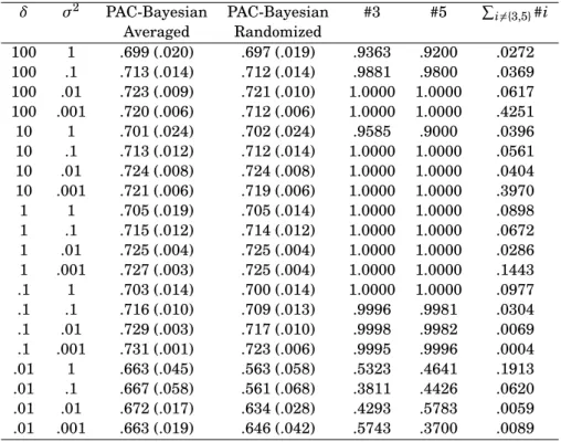
Comments The overall performance is good, and the best AUC value (equal to .731, achieved by the averaged estimator withδ=.1 andσ2=.001) is very close to the optimal oracle value .7387, therefore validating our procedure. As expected, the averaged estimator exhibits slightly better performance (see
Figure 1, a), due to its improved numerical stability over the randomized estimator.
Whenδandσ2are finely calibrated, the algorithm almost always selects the two ground truth covariates (3 and 5, seeFigure 1, b). As highlighted above, additional junk covariates may be selected when the fit to the data is weak (i.e.,δis too small), leading to poor performance.
Table 1: Mean (and variance) of AUC over 50 replications for both estimators (5) and (6) (1000 MCMC iterations, 800 burnin iterations), and frequencies of the selected variables for the last 200 iterations.
δ σ2 PAC-Bayesian PAC-Bayesian #3 #5 P i6={3,5}#i Averaged Randomized 100 1 .699 (.020) .697 (.019) .9363 .9200 .0272 100 .1 .713 (.014) .712 (.014) .9881 .9800 .0369 100 .01 .723 (.009) .721 (.010) 1.0000 1.0000 .0617 100 .001 .720 (.006) .712 (.006) 1.0000 1.0000 .4251 10 1 .701 (.024) .702 (.024) .9585 .9000 .0396 10 .1 .713 (.012) .712 (.014) 1.0000 1.0000 .0561 10 .01 .724 (.008) .724 (.008) 1.0000 1.0000 .0404 10 .001 .721 (.006) .719 (.006) 1.0000 1.0000 .3970 1 1 .705 (.019) .705 (.014) 1.0000 1.0000 .0898 1 .1 .715 (.012) .714 (.012) 1.0000 1.0000 .0672 1 .01 .725 (.004) .725 (.004) 1.0000 1.0000 .0286 1 .001 .727 (.003) .725 (.004) 1.0000 1.0000 .1443 .1 1 .703 (.014) .700 (.014) 1.0000 1.0000 .0977 .1 .1 .716 (.010) .709 (.013) .9996 .9981 .0304 .1 .01 .729 (.003) .717 (.010) .9998 .9982 .0069 .1 .001 .731 (.001) .723 (.006) .9995 .9996 .0004 .01 1 .663 (.045) .563 (.058) .5323 .4641 .1913 .01 .1 .667 (.058) .561 (.068) .3811 .4426 .0620 .01 .01 .672 (.017) .634 (.028) .4293 .5783 .0059 .01 .001 .663 (.019) .646 (.042) .5743 .3700 .0089
We now compare our PAC-Bayesian procedure to two state-of-the-art meth-ods, on real-life datasets. Since our work investigates nonlinear scoring func-tions, we restricted the comparison with similar methods. The Rankboost [19] and TreeRank [7,15] algorithms appear as ideal benchmarks. We have con-ducted a series of experiments on the following datasets: Diabetes, Heart, Iono, Messidor, Pima and Spectf. All these datasets are freely available online, following http://archive.ics.uci.edu/ml/ and serve as classical bench-mark for machine learning tasks. Our results are wrapped up in Table 2
(where TRT, TRl and TRg denote the TreeRank algorithm trained with deci-sion trees, linear SVM and gaussian SVM, respectively). For most datasets, our PAC-Bayesian estimators compete on similar ground with the four other methods, intercalating between the less and most performant method, while being the only ones supported by ground theoretical results.
6
Conclusion
We study in the present paper the problem of bipartite ranking in its the-oretical and algorithmic aspects, in a high-dimensional setting through the PAC-Bayesian approach. Our model is nonlinear and assumes a sparse
addi-Figure 1: Numerical experiments on synthetic data. The two meaningful covariates are the third and the fifth.
(a) Boxplot of AUC for both estimators. Blue dotted line: optimal oracle value (.7387).
PAC−Bayesian Averaged PAC−Bayesian Randomized
0.70
0.71
0.72
0.73
0.74
(b) Selected variables along the MCMC chain.
0 200 400 600 800 1000 2 4 6 8 10 Iterations V ar iab les
(c) For the third covariate, green points are
η(Xi) and red ones aresθˆa(Xi).
0.0 0.2 0.4 0.6 0.8 1.0 −0.2 0.0 0.2 0.4 0.6 0.8 1.0 X3 eta
(d) For the fifth covariate, green points are
η(Xi) and red ones aresθˆa(Xi).
0.0 0.2 0.4 0.6 0.8 1.0 −0.2 0.0 0.2 0.4 0.6 0.8 1.0 X5 eta
tive representation of the optimal scoring function. We propose an estimator based on the Gibbs pseudo-posterior distribution, and derive oracle inequal-ities in probability under the sparsity assumption,i.e., with terms involving the intrinsic dimension instead of the ambient dimensiond. Under minimal assumption, we recover classical rates of convergenceO(n−1/2). On a Sobolev ellipsoid with regularityτand under a margin assumption of parameterα, we obtain the minimax rate of convergenceO³n−(11++(2τ(1+α+)ατ))´. A salient fact is that
our results significantly extend previous works [12], in that our inequalities hold in probability (instead of inequalities in expectation). A summary of all our theoretical claims is presented inTable 3.
Next, we propose an implementation of the PAC-Bayesian estimators through a transdimensional MCMC. Its performance on synthetic and real-life datasets
Table 2: Cross-validated mean (and variance) of AUC over seven real-life datasets.
Name (n,d) PAC-B. PAC-B. TRT TRl TRg Rankboost Averaged Randomized Vowel (990,10) .848 (.018) .846 (.017) .908 (.017) .946 (.011) .976 (.009) .946 (.013) Messidor (1151,11) .738 (.033) .732 (.034) .687 (.038) .800 (.023) .754 (.036) .747 (.021) Iono (351,32) .871 (.047) .869 (.047) .878 (.033) .846 (.050) .905 (.024) .929 (.017) Diabetes (768,8) .772 (.038) .767 (.040) .777 (.037) .810 (.036) .794 (.037) .820 (.033) Heart (270,5) .733 (.061) .725 (.065) .700 (.072) .752 (.063) .676 (.077) .746 (.062) Pima (768,8) .782 (.036) .772 (.038) .777 (.037) .810 (.036) .703 (.033) .820 (.033) Spectf (267,44) .764 (.103) .759 (.102) .757 (.129) .711 (.109) .601 (.089) .854 (.111)
Table 3: Summary of the theoretical results.
Result Ass.1 Ass.2 Ass.3 Comment
Theorem 1 Most generic result
Theorem 2 3 With a sparsity-inducing prior
Theorem 3 3 Faster rates with margin assumption, generic prior
Theorem 4 3 3 Faster rates with margin assumption, sparsity-inducing prior
Theorem 5 3 3 On Sobolev spaces, no margin assumption
Theorem 6 3 3 3 On Sobolev spaces, with a margin assumption
competes with other nonlinear ranking algorithms. In conclusion, the main contributions of this paper are a nonlinear procedure with provable minimax rates and an efficient implemented approximation for the bipartite ranking problem.
7
Proofs
The following lemma [Legendre transform of the Kullback-Leibler divergence, 16] is a key ingredient in our proofs and the demonstration may be found in [10, Equation 5.2.1].
Lemma 2. Let(A,A)be a measurable space. For any probabilityµon(A,A)
and any measurable function h:A→Rsuch thatR
(exp◦h)dµ< ∞, log Z (exp◦h)dµ= sup m∈M1+,π(A,A) ½Z hdm−K(m,µ) ¾ ,
with the convention∞ − ∞ = −∞. Moreover, as soon as h is upper-bounded on the support ofµ, the supremum with respect to m on the right-hand side is reached for the Gibbs distribution g given by
dg
dµ(a)=
exp◦h(a) R
(exp◦h)dµ, a∈A.
Proof ofTheorem 1. Assume that (3) holds. For anyε∈(0, 1), we have
Eexp£
Now, assume thatsis drawn from some prior distributionπ. We can integrate on both sides of the previous inequality, thus
Z ©
Eexp£
δ(En(s)−E(s))−ψ(s)−log(1/ε)¤ªπ(ds)≤ε. Using a Fubini-Tonelli theorem, we may write
EZ exp£
δ(En(s)−E(s))−ψ(s)−log(1/ε)¤π(ds)≤ε.
Now, letρdenote an absolutely continuous distribution with respect toπ. We obtain EZ exp · δ(En(s)−E(s))−ψ(s)−log dρ dπ(s)−log(1/ε) ¸ ρ(ds)≤ε.
With a slight extension of previous notation, we letE stands for the expec-tation computed with respect to the distribution of (X,Y) and the posterior distributionρ. Using the elementary inequality exp(δx)≥1R+(x),
P " En(s)−E(s)− ψ+log(1/ε)+logddρπ(s) δ >0 # ≤ε, i.e., P " En(s)≤E(s)+ ψ(s)+log(1/ε)+logddρπ(s) δ # ≥1−ε. (8)
We may now apply the same scheme of proof with the variablesTei,j= −Ti,j to obtain P " E(s)≤En(s)+ ψ(s)+log(1/ε)+logddρπ(s) δ # ≥1−ε. Now, for the choiceρ=ρˆδand ˆs∼ρˆδ,
P " E( ˆs)≤En( ˆs)+ ψ( ˆs)+log(1/ε)+logd ˆdρπδ( ˆs) δ # ≥1−ε. Note that logd ˆρδ dπ( ˆs)=log exp(−δLn( ˆs)) R exp(−δLn(s0))π(ds0)= −δLn( ˆs)−log Z exp¡ −δLn(s0)¢π(ds0). Hence P · E( ˆs)≤ −Ln(η)+1 δ µ ψ( ˆs)+log(1/ε)−log Z exp(−δLn(s0))π(ds0) ¶¸ ≥1−ε. FromLemma 2, we obtain
P · E( ˆs)≤ inf ρ∈Mπ ½Z En(s)ρ(ds)+ψ ( ˆs)+log(1/ε)+K(ρ,π) δ ¾¸ ≥1−ε,
wheres∼ρ. So by integrating (8), P · E( ˆs)≤ inf ρ∈Mπ ½Z E(s)ρ(ds)+ Z ψ(s) δ ρ(ds)+ ψ( ˆs)+2 log(2/ε)+2K(ρ,π) δ ¾¸ ≥1−ε, (9) which is the desired result.
Proof ofLemma 1. For some candidate function sand any i,j=1, . . . ,n, de-fine
Ti,j=1{(s(Xi)−s(Xj))(Yi−Yj)<0}−1{(η(Xi)−η(Xj))(Yi−Yj)<0}.
Using results on U-statistics [Hoeffding decomposition of U-statistics,33], we may write, for anyγ>0,
Eexp " γX i6=j (Ti,j−ETi,j) # =Eexp " γn(n−1) n! X π 1 n/2 n/2 X i=1 (Tπ(i),π(i+n/2)−ETπ(i),π(i+n/2)) # ≤Eexp " 2γ(n−1) n/2 X i=1 (Ti,i+n/2−ETi,i+n/2) # , (10)
where we used the Jensen’s inequality. Next, using an independence argu-ment and Hoeffding’s inequality applied to the random variable Ti,i+n/2−
ETi,i+n/2∈(−ETi,i+n/2, 1−ETi,i+n/2), Eexp " γX i6=j (Ti,j−ETi,j) # = n/2 Y i=1 Eexp£ 2γ(n−1)(Ti,i+n/2−ETi,i+n/2)¤ ≤ n/2 Y i=1 exp µγ2(n −1)2 2 ¶ =exp µnγ2(n −1)2 4 ¶ =exp(ψ), withψ=δ2/4nandδ=γn(n−1). Note thatψdoes not depend ons. Finally, note that Eexp " γX i6=j (Ti,j−ETi,j) # =Eexp [δ(En(s)−E(s))] .
Proof ofTheorem 2. FromTheorem 1and sinceψ=δ2/4ndoes not depend on
s, consideringρmas a probability measure whose support isR|m|0,
P · E( ˆs)≤inf m infρm ½Z E(s)ρ(ds)+2ψ+2 log(2/ε)+2K(ρm,π) δ ¾¸ ≥1−ε. Next, note that
K(ρm,π)=K(ρm,πm)+ |m|0Mlog(1/β)+log à d |m|0 ! +log1−β d+1 1−β ≤K(ρm,πm)+ |m|0Mlog(1/β)+ |m|0log d e |m|0+ log 1 1−β, (11)
where we used the elementary inequality log¡d k ¢
≤klogd ek . Note that if we consider as distributions ρm uniform distributions on `2-balls centered in anyθ∈Bmsuch thatkθk =1, of radiust∈(0, 1), we obtain thatK(ρm,πm)= |m|0log(1/t). For someθ0such thatkθ0k =1,
R(sθ)=E[1{(sθ(X)−sθ(X0))(Y−Y0)<0}] =E[1{(sθ0(X)−sθ0(X0))(Y−Y0)<0}] +E[1{(sθ(X)−sθ(X0))(Y−Y0)<0}−1{(sθ 0(X)−sθ0(X0))(Y−Y0)<0}] ≤R(sθ0)+P[sign(sθ(X)−sθ(X0))(Y−Y0))6=sign(sθ0(X)−sθ0(X0))(Y−Y0)] =R(sθ0)+P[sign(sθ(X)−sθ(X0))6=sign(sθ0(X)−sθ0(X0))] ≤R(sθ0)+2ckθ−θ0k,
where we used Assumption 1in the last inequality. Let ρm,θ0,t denote the
uniform distribution on the`2-ball centered inθ0and of radiust∈(0, 1). From what precedes,
Z
E(sθ)ρm,θ0,t(ds)=R(sθ0)+2ct. (12)
Using the notation
K=2 µ |m|0Mlog(1/β)+ |m|0log d e |m|0+ log 1 1−β ¶ , (13) we obtain P · E( ˆs)≤inf m θ∈Bminf,kθk=1 t∈inf(0,1) ½ R(sθ0)+2ct +2ψ+2 log(2/ε)+2|m|0log(1/t)+2K δ ¾¸ ≥1−ε. It can easily be seen that the functiont7→2ct+log(1/t)/δis upper-bounded at the pointt=1/(2cδ). Therefore,
P · E( ˆs)≤inf m θ∈Bminf,kθk=1 ½ R(sθ0)+1+2ψ+2 log(2/ε)+2|m|0log(2cδ)+2K δ ¾¸ ≥1−ε. Now, recalling thatψ=δ2/4n, we chooseδ=pn. The desired result is then straightforward from the proof ofTheorem 1.
The followingLemma 3allows us to obtain a tighter right-hand term in (3), therefore leading to a refined oracle inequality with a faster rate of conver-gence. Let us introduce the notationφ(u)=eu−u−1.
Lemma 3. Let s be a scoring function and(X,Y)and(X0,Y0)two pairs of inde-pendent random variables. Let T(s)=1{(s(X)−s(X0))(Y−Y0)<0}−1{(η(X)−η(X0))(Y−Y0)<0},
andV(Z)denote the variance of a random variable Z. LetAssumption 2hold for someα∈(0, 1), then
V(T(s))≤C(L(s)−L∗)1+αα,
where C is a constant. Hence, for any distribution of the random variables
(X,Y) satisfying Assumption 2 for some parameter α∈(0, 1), (3) holds with
ψ(s)=n2V(T(s))φ³2nδ´.
Proof ofLemma 3. First, note thatET=L(s)−L?≥0. Let
r=r(X,X0)=sign(s(X)−s(X0)), r?=r?(X,X0)=sign(η(X)−η(X0)), Z=(Y−Y0)/2. With this notation,
ET2=E£ 1{r6=Z}+1{r?6=Z}−21{r6=Z}1{r?6=Z} ¤ =E£1{r=1}1{Z=−1}+1{r=−1}1{Z=1}+1{r?=1}1{Z=−1}+1{r?=−1}1{Z=1} −21{r=1}1{r?=1}1{Z=−1}−21{r=−1}1{r?=−1}1{Z=1}¤. Next, ET2=E£ 1{r=1}(1−η(X))η(X0)+1{r=−1}η(X)(1−η(X0))+1{r?=1}(1−η(X))η(X0) +1{r?=−1}η(X)(1−η(X0))−21{r=1}1{r?=1}(1−η(X))η(X0) −21{r=−1}1{r?=−1}η(X)(1−η(X0))¤. Thus, ET2=E£ (1−η(X))η(X0)(1{r=1}+1{r?=1}−21{r=1}1{r?=1}) +η(X)(1−η(X0))(1{r=−1}+1{r?=1}−21{r=−1}1{r?=−1})¤ =E£1{r6=r?}((1−η(X))η(X0)+η(X)(1−η(X0))) ¤ =E£1{r6=r?}(η(X)+η(X0)−2η(X)η(X0))¤ ≤1 2E £ 1{r6=r?} ¤ ≤1 2C(L(s)−L ?)α/(1+α). Finally, V(T)=ET2−(ET)2≤C(L(s)−L?)α/(1+α), whereCis a constant, which proves the first statement.
Recalling (10), with the notationφ(u)=eu−u−1 and Benett’s inequality, we get Eexp " γX i6=j ¡ Ti,j(s)−ETi,j(s)¢ # ≤ n/2 Y i=1 exp¡ V¡ Ti,i+n/2(s)¢φ¡2(n−1)γ¢¢ =exp³n 2V(T(s))φ(2(n−1)γ) ´ ,
withγ=n(nδ
−1), which yields
Eexp [δ(En(s)−E(s))]≤exp(ψ),
withψ=n2V(T(s))φ³2nδ´, achieving the second statement ofLemma 3.
Proof ofTheorem 3. Now, combining what precedes and (9),
P · E( ˆs)≤ inf ρ∈Mπ ½Z E(s)ρ(ds)+ Z nV(T(s))φ(2δ/n) 2δ ρ(ds) +nV(T( ˆs))φ(2δ/n) /2+2 log(2/ε)+2K(ρ,π) δ ¾¸ ≥1−ε. Using the elementary inequalityφ(x)/x≤xfor anyx∈(0, 1) yields
P · E( ˆs)≤ inf ρ∈Mπ ½Z E(s)ρ(ds)+ Z 2δV(T(s)) n ρ(ds)+ 2δV(T( ˆs)) n +2 log(2/ε)δ+2K(ρ,π) ¾¸ ≥1−ε. Now, usingLemma 3,
P " E( ˆs)≤ inf ρ∈Mπ ( Z E(s)ρ(ds)+ Z 2δCE(s)1+αα n ρ(ds)+ 2δCE( ˆs)1α+α n +2 log(2/ε)+2K(ρ,π) δ ¾¸ ≥1−ε. Thus, for anyx≥0,
P ·µ 1−2δCx n ¶ E( ˆs)≤ inf ρ∈Mπ ½Z µ 1+2δCx n ¶ E(s)ρ(ds) + Z 2δC n ³ E(s)1+αα−xE(s) ´ ρ(ds)+2δC n ³ E( ˆs)1+αα−xE( ˆs) ´ +2 log(2/ε)+2K(ρ,π) δ ¾¸ ≥1−ε. Clearly, the functiont7→t1α+α−xtis upper bounded byx−α1+α1 ¡ α
1+α ¢α , so P ·µ 1−2δCx n ¶ E( ˆs)≤ inf ρ∈Mπ ½Z µ 1+2δCx n ¶ E(s)ρ(ds) + Z 2δCC α n x −αρ(ds)+2δCCα n x −α+2 log(2/ε)+2K(ρ,π) δ ¾¸ ≥1−ε, (14) whereCα=1+α1 ¡ α 1+α ¢α
. Next, we choosex=4δnC. The functionδ7→Cα³4nC´1+αδ1+α+ 4
δis upper-bounded at the pointδ=Υn 1+α 2+α whereΥ=2((1+α)Cα)−2+1α(2C)−12++αα. Thus we obtain P · E( ˆs)≤ inf ρ∈Mπ ½ 3 Z E(s)ρ(ds)+n−12++αα£Cα(CΥ)1+α+Υ−1¡log(2/ε)+K(ρ,π)¢¤ ¾¸ ≥1−ε.
Proof ofTheorem 4. Note that from (14), choosingx=4nδC, we get P " E( ˆs)≤inf m infρm ( 3 Z E(s)ρ(ds)+2Cα µ4δC n ¶1+α +4 log(2/ε)+δ4K(ρm,π) )# ≥1−ε. Now, recall the result from (11).
P " E( ˆs)≤inf m θ∈Bminf,kθk=1t∈inf(0,1) ( 3 Z E(sθ)ρm,θ,t(ds)+2Cα µ4δC n ¶1+α +4 log(2/ε) δ +4|
m|0log(1/t)+ |m|0Mlog(1/β)+ |m|0log|md e|0+log1−β1
δ
)#
≥1−ε. With the notation stated in (13) and the result (12),
P " E( ˆs)≤inf m θ∈Bminf,kθk=1t∈inf(0,1) ( 3E(sθ)+4ct+2Cα µ4δC n ¶1+α +4 log(2/ε) δ +4|m|0log(1/t)+K δ ¾¸ ≥1−ε. Sincet7→4ct+log(1/t)/δis upper-bounded at the pointt=1/(4cδ),
P " E( ˆs)≤inf m θ∈Bminf,kθk=1 ( 3E(sθ)+2Cα µ4δC n ¶1+α +4 log(2/ε) δ +4|m|0log(4cδ)+K δ ¾¸ ≥1−ε. (15) Finally, noticing that the functionδ7→Cα³4δnC´1+α+1δis upper-bounded at the pointδ=n12++αα¡1 4C ¢12++αα³ 1 Cα(1+α) ´2+1α , we obtain P E( ˆs)≤infm θ∈Binf m,kθk=1 ½ 3E(sθ) +n−12++αα(4K+4 log(2/ε)+log(4cn12++αα))C 1 2+α α µ 1 4C ¶−12++ααh (1+α)−12++αα+(1+α)2+1α i¾ ≥1−ε.
Proof ofTheorem 5. We denote byηprojthe projection ofηontoSΘ. LetΓηproj=
© (x,x0)|¡ ηproj(x) −ηproj(x0)¢ ¡ η(x)−η(x0)¢ <0ª
. For any X,X0 ∈Γηproj, we have
that|η(X)−η(X0)| ≤ |ηproj(X)−η(X)| + |ηproj(X0)−η(X0)|. Since [see14]
L³ηproj´−L?=Eh|η(X)−η(X0)|1{(X,X0)∈Γηproj}
i ,
we obtainL(ηproj)−L?≤2E[|ηproj(X)−η(X)|]. Next, using the statement (11) combined withTheorem 1, result (12) and the choiceψ=δ2/4n (which holds whatever the distribution of (X,Y) may be), we get that
P · E( ˆs)≤inf m θ∈Bminf,kθk=1 t∈inf(0,1) ½ E(sθ)+2ct+ δ 2n+ 2 log(2/ε)+ |m|0log(1/t)+2K δ ¾¸ ≥1−ε, whereK= |m|0Mlog(1/β)+ |m|0log|md e|0+log1−β1 . Since the functiont7→2ct+ log(1/t)/δis upper-bounded at the pointt=1/(2cδ), hence
P · E( ˆs)≤inf m θ∈Bminf,kθk=1 ½ E(sθ)+ δ 2n+ 1+2 log(2/ε)+ |m|0log(2cδ)+2K δ ¾¸ ≥1−ε, Now, inf θ∈Bm,kθk=1 E(sθ)=E(ηproj)≤2E|ηproj(X)−η(X)| ≤2 q E|ηproj(X)−η(X)|2 ≤2 sZ X j∈S? X k≥M+1 |θ?jk|2φ2 k(x)µ(dx) ≤2pB s X j∈S? X k≥M+1 |θ? jk|2,
since the φk’s are such that R|φk(x)|µ(dx)≤B where B>0 is a numerical constant. Using the definition of the Sobolev ellipsoid, we obtain
inf θ∈Bm,kθk=1 E(sθ)≤2pB|S?|0κ(1+M)−τ. Hence P · E( ˆs)≤inf m ½ 2pBκ|S?|0(1+M)−τ+ δ 2n+ |m|0Mlog(1/β) δ +1+ |m|0log(2cδ)+2 log(2/ε)+2K 0 δ ¾¸ ≥1−ε, whereK0= |m|0log|md e|0+log1−β1 . Next, observe that we get rid of the remain-ing infimum by substitutremain-ing|S?|to|m|0.
The function t7→2pBκ|S?|0(1+t)−τ+ |S?|0log(1/β)t/δ is upper-bounded at the pointt= µp |S?|0log(1/β) 2pBκτδ ¶−11+τ −1, which yields P · E( ˆs)≤ ½ ζδ1−+ττ+ δ 2n+ 1+2 log(2/ε)+2K0| + |S?|0log(2cδ) δ ¾¸ ≥1−ε,
whereζ= µ ³ 2pBκ´ 1 1+τ |S?| 1+2τ 2+2τ 0 log(1/β) τ 1+τ ³ τ−1+ττ+τ1+1τ ´¶ , andK0= |S?| 0log|Sd e?|0+ log1−β1 . Since t7→ζt−1+ττ+ t
2n is upper-bounded at the pointt=n
τ+1 2τ+1 ³2ζτ 1+τ ´2ττ++11 , P " E( ˆs)≤ ( ζ µ2ζτn 1+τ ¶2ττ+1 +1×1−+ττ + 1 2n µ2ζτn 1+τ ¶2ττ+1 +1 +¡2 log(2/ε)+2K0+ |S?|0log(2cδ)¢ µ2ζτn 1+τ ¶−2ττ++11)# ≥1−ε. Finally, P " E( ˆs)≤ ( ξn−2ττ+1+(2 log(2/ε)+2K0+ |S?|0log(C1n τ+1 2τ+1)) µ2ζτn 1+τ ¶−2ττ+1 +1)# ≥1−ε, whereξ=ζ2ττ++112− τ 2τ+1 ³¡ τ 1+τ ¢−2ττ +1+¡ τ 1+τ ¢2ττ+1 +1´andC 1=2c ³2ζτ 1+τ ´2ττ++11 .
Proof ofTheorem 6. Observe that [as written in12, Proposition 4] inf
θ∈Bm,kθk=1
E(sθ)=E(ηproj)
≤2kηproj−ηk∞Ph³ηproj(X)−ηproj(X0)´¡
η(X)−η(X0)¢
<0i
≤2Ckηproj−ηk∞E(ηproj)1+αα (byAssumption 2).
Hence, E(ηproj)≤³2Ckηproj−ηk∞ ´1+α ≤(2C)1+α Ã sup x X j∈S? X k≥M+1 θjkφk(xj) !1+α ≤(2BC)1+α Ã X j∈S? X k≥M+1 |θjk| !1+α ≤³2BCpκ|S?|0´1+α(1+M)−τ(1+α), by construction of theφk’s. Combining (15) with what precedes, we get
P " E( ˆs)≤2 ( 3 2 ³ 2BCpκ|S?|0 ´1+α (1+M)−τ(1+α)+ µ4Cδ n ¶1+α +|S ?| 0Mlog(1/β) δ + 2 log(2/ε)+2K0+ |S?|0log(2cδ) δ ¾¸ ≥1−ε, The functiont7→3/2³2BCpκ|S?|0 ´1+α (1+t)−τ(1+α)+|S?|0log(1/β)t/δis upper-bounded at the pointt=
à 2|S?|0log(1/β) 3τ(1+α)³2BCpκ|S?|0 ´1+α δ !−1+τ(11+α) −1, so we may write P " E( ˆs)≤2 ( ζδ1−+ττ(1(1++αα))+ µ4Cδ n ¶1+α +2 log(2/ε)+2K 0+ |S?| 0log(2cδ) δ )# ≥1−ε,
where ζ= µ 3/2³2BCpκ|S?|0 ´1+α¶ 1 1+τ(1+α) ¡ log(1/β)|S?|0¢ τ(1+α) 1+τ(1+α) ׳(τ(1+α))−1+τ(1τ(1++αα))+(τ(1+α)) 1 1+τ(1+α) ´ . The function t7→ζt−1+τ(1τ+α)+ ³4Ct n ´1+α
(it is sufficient to consider this part) is upper-bounded at the pointt=³1ζτ+τ(1(1+α+α))´
1+τ(1+α) (1+τ(2+α))(1+α)¡ n 4C ¢11++ττ(1(2++αα)) , hence using the notationΥ=³1ζτ+τ(1(1+α+α))´ 1+τ(1+α) (1+τ(2+α))(1+α)¡ 1 4C ¢11++ττ(1(2++αα)) , we obtain that PhE( ˆs)≤2n³ζΥ−1+τ(1τ(1++αα))+(4CΥ)1+α ´ n1−+τ(2(1++αα))τ +Υ−1n−1(1++(2τ+(1α+)ατ))(2 log(2/ε)+2K0+ |S?|0log(2cΥn11++ττ(1(2++αα)))) oi ≥1−ε.
Acknowledgements
The authors would like to thank the Associate Editor and a Reviewer for valuable comments and insightful suggestions, which led to a substantial improvement of the paper.
References
[1] S. Agarwal, T. Graepel, R. Herbrich, S. Har-Peled, and D. Roth. Generalization bounds for the Area Under the ROC Curve. Journal of Machine Learning Research, 6:393–425, 2005.
[2] P. Alquier. PAC-Bayesian Bounds for Randomized Empirical Risk Minimizers. Mathe-matical Methods of Statistics, 17(4):279–304, 2008.
[3] P. Alquier and G. Biau. Sparse Single-Index Model. Journal of Machine Learning Re-search, 14:243–280, 2013.
[4] P. Alquier and K. Lounici. PAC-Bayesian Theorems for Sparse Regression Estimation with Exponential Weights. Electronic Journal of Statistics, 5:127–145, 2011. doi: 10. 1214/11-EJS601.
[5] J.-Y. Audibert. Aggregated estimators and empirical complexity for least square regres-sion. Annales de l’Institut Henri Poincaré : Probabilités et Statistiques, 40(6):685–736, November-December 2004.
[6] J.-Y. Audibert and A. B. Tsybakov. Fast learning rates for plug-in classifiers.The Annals of Statistics, 35(2):608–633, 2007.
[7] N. Baskiotis, S. Clémençon, M. Depecker, and N. Vayatis. TreeRank: an R package for bipartite ranking. InProceedings of SMDTA 2010 - Stochastic Modeling Techniques and Data Analysis International Conference, 2010.
[8] S. Boucheron, O. Bousquet, and G. Lugosi. Theory of classification: a survey of some recent advances.ESAIM: Probability and Statistics, 9:323–375, 2005.
[9] B. P. Carlin and S. Chib. Bayesian Model choice via Markov Chain Monte Carlo Methods. Journal of the Royal Statistical Society, Series B, 57(3):473–484, 1995.
[10] O. Catoni. Statistical Learning Theory and Stochastic Optimization. École d’Été de Probabilités de Saint-Flour XXXI – 2001. Springer, 2004.
[11] O. Catoni. PAC-Bayesian Supervised Classification: The Thermodynamics of Statistical Learning, volume 56 ofLecture notes – Monograph Series. Institute of Mathematical Statistics, 2007.
[12] S. Clémençon and S. Robbiano. Minimax learning rates for bipartite ranking and plug-in rules. InProceedings of the 28th ICML, pages 441–448, 2011.
[13] S. Clémençon and N. Vayatis. Tree-based ranking methods.IEEE Transactions on Infor-mation Theory, 55(9):4316–4336, 2009.
[14] S. Clémençon, G. Lugosi, and N. Vayatis. Ranking and empirical risk minimization of U-statistics.The Annals of Statistics, 36:844–874, 2008.
[15] S. Clémençon, M. Depecker, and N. Vayatis. Adaptive partitioning schemes for bipartite ranking: How to grow and prune a ranking tree.Machine Learning, 83(1):31–69, 2011. [16] I. Csiszár.i-divergence geometry of probability distributions and minimization problems.
The Annals of Probability, 3:146–158, 1975.
[17] A. S. Dalalyan and A. B. Tsybakov. Aggregation by exponential weighting, sharp PAC-Bayesian bounds and sparsity. Machine Learning, 72(1-2):39–61, 2008. doi: 10.1007/ s10994-008-5051-0.
[18] A. S. Dalalyan and A. B. Tsybakov. Sparse Regression Learning by Aggregation and Langevin Monte-Carlo. Journal of Computer and System Sciences, 78(5):1423–1443, 2012. doi: 10.1016/j.jcss.2011.12.023.
[19] Y. Freund, R. D. Iyer, R. E. Schapire, and Y. Singer. An efficient boosting algorithm for combining preferences.Journal of Machine Learning Research, 4:933–969, 2003. [20] D. M. Green and J. A. Swets.Signal detection theory and psychophysics. Wiley, 1966. [21] B. Guedj.pacbpred: PAC-Bayesian Estimation and Prediction in Sparse Additive Models,
February 2013. URLhttp://cran.r-project.org/web/packages/pacbpred/index. html. R package version 0.92.2.
[22] B. Guedj and P. Alquier. PAC-Bayesian estimation and prediction in sparse additive models.Electronic Journal of Statistics, 7:264–291, 2013. ISSN 1935-7524. doi: 10.1214/ 13-EJS771.
[23] T. Hastie and R. Tibshirani. Generalized Additive Models.Statistical Science, 1(3):297– 318, 1986.
[24] G. Lecué. Optimal oracle inequality for aggregation of classifiers under low noise condi-tion. InProceedings of the 19th COLT, pages 364–378, 2006.
[25] G. Leung and A. R. Barron. Information theory and mixing least-squares regressions. IEEE Transactions on Information Theory, 52(8):3396–3410, August 2006. doi: 10.1109/ TIT.2006.878172.