Generalized differential morphological profiles for remote sensing image classification

For Review Only

Generalized Differential Morphological Profiles for Remote Sensing Image Classification

Journal: Journal of Selected Topics in Applied Earth Observations and Remote

Sensing

Manuscript ID JSTARS-2015-00722 Manuscript type: Regular

Date Submitted by the Author: 22-Sep-2015

Complete List of Authors: Huang, Xin; Wuhan University, School of Remote Sensing and Information Engineering

Han, Xiaopeng; Wuhan University, The State Key Laboratory of Information Engineering in Surveying, Mapping, and Remote Sensing

Liu, Hui; Wuhan University, The State Key Laboratory of Information Engineering in Surveying, Mapping, and Remote Sensing

Zhang, Liangpei; Wuhan University, The State Key Laboratory of Information Engineering in Surveying, Mapping, and Remote Sensing Liao, Wenzhi; Ghent University, Department of Telecommunications and Information Processing

Benediktsson, Jon Atli; University of Iceland, Engineering Research Institute;

Keywords: Feature extraction

For Review Only

Generalized Differential Morphological Profiles for Remote Sensing Image

Classification

Xin Huang, Senior Member, IEEE, Xiaopeng Han, Hui Liu, Liangpei Zhang, Senior Member, IEEE, Wenzhi Liao, Member, IEEE, and Jon Atli Benediktsson, Fellow, IEEE

Abstract—Differential morphological profiles (DMPs) are widely used for the spatial/structural feature

extraction and classification of remote sensing images. They can be regarded as the shape spectrum, depicting the response of the image structures related to different scales and sizes of the structural elements (SEs). DMPs are defined as the difference of morphological profiles (MPs) between consecutive scales. However, traditional DMPs can ignore discriminative information for features that are across the scales in the profiles (“accross-scale” features). To solve this problem, we propose scale-span differential profiles, i.e., generalized differential morphological profiles (GDMPs), to obtain the entire differential profiles. GDMPs can describe the complete shape spectrum and measure the difference between arbitrary scales, which is more appropriate for representing the multiscale characteristics and complex landscapes of remote sensing image scenes. Subsequently, the random forest (RF) classifier is applied to interpret GDMPs considering its robustness for high-dimension data and ability of evaluating the importance of variables. Meanwhile, the random forest “Out-of-Bag” error can be used to quantify the importance of each channel of GDMPs and

select the most discriminative information in the entire profiles. Experiments conducted on three well-known hyperspectral data sets as well as an additional WorldView-2 data are used to validate the effectiveness of GDMPs compared to the traditional DMPs. The results are promising as GDMPs can significantly outperform the traditional one, as it is capable of adequately exploring the multiscale morphological information.

Index Terms—Morphological profiles, feature selection, feature extraction, Random Forest (RF), classification. 1 2 3 4 5 6 7 8 9 10 11 12 13 14 15 16 17 18 19 20 21 22 23 24 25 26 27 28 29 30 31 32 33 34 35 36 37 38 39 40 41 42 43 44 45 46 47 48 49 50 51 52 53 54 55 56 57 58 59 60

For Review Only

I. INTRODUCTION

Advances in Earth observation technology, leading to an increased availability of data from different sensors, has opened up new avenues for geospatial information extraction. Recently, remote sensing data can provide wealthy information in spatial domains. However, higher spatial resolution does not naturally correspond to higher image interpretation accuracies, and their availability poses challenges to land cover and land use mapping, especially in urban areas. Due to the complex spatial arrangement and spectral heterogeneity even within the same class, conventional spectral-based classification suffers from a large number of misclassifications between spectrally similar classes [1]. Moreover, high spatial resolution images are subject to increase of the intra-class variance and decrease of the inter-class variance in the spectral feature space, leading to decreased class separability in the spectral domain [2]. Therefore, there is an increased interest and demand in incorporating geometrical information into the image classification. Specifically, in recent years, a few studies on spectral-spatial joint feature extraction and classification have been proposed. One of the state-of-the-art procedures for spatial feature is the gray level co-occurrence matrix (GLCM) [3], which is a widely used texture and pattern recognition technique in the analysis of remote sensing data. For instance, recently, a GLCM based on the sparse coding was proposed for hyperspectral texture representation and achieved higher classification accuracy compared to the original GLCM [4]. The Markov random-field is also an effective way to take into account spatial information for image interpretation [5]. Other commonly used spatial features include Wavelet transform (WT) [6], pixel shape index (PSI) [7], Local Binary Pattern (LBP) [8] [9], etc., aiming to explore the spatial correlation and structural information for enhancing the traditional spectral-based image classification.

Recently, mathematical morphology, which can effectively explore the spatial and structural information from the remote sensing data, has received more and more attention. In [10], differential morphological profiles (DMPs) were proposed and applied to remote sensing image segmentation and classification. In

1 2 3 4 5 6 7 8 9 10 11 12 13 14 15 16 17 18 19 20 21 22 23 24 25 26 27 28 29 30 31 32 33 34 35 36 37 38 39 40 41 42 43 44 45 46 47 48 49 50 51 52 53 54 55 56 57 58 59 60

For Review Only

particular, the segmentation map was obtained by associating each pixel to the level where the DMP value of corresponding pixel reaches the maximum. In [11], dimensionality reduction, e.g., feature extraction and feature selection were applied to the DMPs, and the dimensionally reduced profiles were then fed into a neural network classifier for image classification. DMPs were further investigated in [12], where they were interpreted in terms of a fuzzy measurement of the characteristic size and contrast of each structure. The fuzzy measure was compared to a set of predefined possibility distributions to derive a membership degree for various land cover classes. Morphological texture features were applied to mangrove forest mapping and species discrimination in [13]. MPs can be extended for representing image structures for hyperspectral images [14], where MPs are computed on the first few principal components of hyperspectral data, called extended morphological profiles (EMPs). More recently, morphological attribute profiles (APs) were proposed, providing a variety of attributes (e.g., area, volume, moment of inertia) based on a multilevel characterization of an image using connected operators [15]. In [16], [17], extended attribute profiles (EAPs) were presented by calculating the APs on the independent components of hyperspectral data. Furthermore, a set of new multiple morphological profiles (MMPs) were created by integrating the MPs derived from multiple base images produced by various strategies, including linear, nonlinear, multi-linear image transformation and manifold learning methods [18]. A survey on the spectral-spatial classification techniques based on morphological profiles can be found in [19].

Among these morphological profiles, differential morphological profiles (DMPs), regarded as the shape spectrum of objects, have been proved effective in describing the structural and spatial features from remote sensing images and achieved promising performances. DMPs are constructed on the repeated use of openings and closings by a series of structuring element (SE) with increasing sizes. However, traditional DMPs focus on the differences between consecutive scales with a constant interval, which actually ignore the arbitrary information in the profiles that are accross-scale and lead to underutilization of the

discriminative features. To address this problem, generalized differential morphological profiles (GDMPs)

1 2 3 4 5 6 7 8 9 10 11 12 13 14 15 16 17 18 19 20 21 22 23 24 25 26 27 28 29 30 31 32 33 34 35 36 37 38 39 40 41 42 43 44 45 46 47 48 49 50 51 52 53 54 55 56 57 58 59 60

For Review Only

are proposed in this research. The notable advantage of the GDMPs is that it can describe the entire shape spectrum between two arbitrary scales from the morphological profiles, which is actually more appropriate for representing the multiscale characteristics and complex landscapes of remote sensing image scenes.

Furthermore, considering the high-dimensional feature space and redundant information caused by GDMPs, in this study, random forest is employed for interpreting GDMPs, i.e., in classification. The importance of each element in the entire profiles can be quantified by using the “Out-of-Bag” analysis [20],

[21]. In this way, the feature selection is performed and larger weights are given to the more discriminative features in the profiles.

In this study, in order to adequately verify the effectiveness of the GDMPs, both geodesic morphological reconstruction [22], [10]-[12] and partial morphological reconstruction [23] [24] are employed for constructing the GDMPs. In particular, the partial reconstruction can preserve the shape of objects as much as possible, and suppress the “over-reconstruction” problem.

In the experimental section, the proposed GDMPs are validated on four widely used and public remote sensing data sets: HYDICE DC Mall, ROSIS Pavia University, AVIRIS Indian pines and Worldview-2 Hainan, respectively.

The remainder of this paper is organized as follows. Section II briefly introduces the principles of GDMPs using geodesic and partial reconstruction respectively, followed by introduction of RF classifier for GDMPs feature selection and classification. Experimental results and the corresponding analysis are presented in section III, and Section IV concludes this study with some remarks and hints at plausible future research.

1 2 3 4 5 6 7 8 9 10 11 12 13 14 15 16 17 18 19 20 21 22 23 24 25 26 27 28 29 30 31 32 33 34 35 36 37 38 39 40 41 42 43 44 45 46 47 48 49 50 51 52 53 54 55 56 57 58 59 60

For Review Only

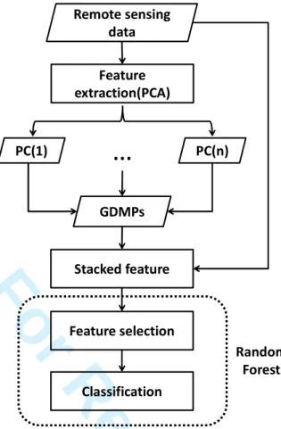
Fig. 1. General workflow of this study.

II.METHODDOLOGY

Erosion and dilation are the basic operators of mathematical morphological [25]. The operators are applied to an image with a set of known shapes (e.g., disk, square), called structuring elements (SEs). Erosion and dilation can be used to define the commonly used morphological operators: opening and closing. Morphological opening is to dilate an eroded image aiming at isolating bright structures, and closing is to erode a dilated image for suppressing dark structures. In order to preserve the shape of the objects and introduce less shape noise, geodesic reconstruction [22], [10]-[12] and partial reconstruction [23] are used. The proposed GDMPs are defined on the basis of the aforementioned morphological processing. The processing chain of the GDMPs is shown in Fig. 1. Note that in this paper, both GDMPs with geodesic reconstruction and partial reconstruction are investigated.

A. GDMPs

MPs [14], [26] are implemented on a series of morphological openings and closings with a family of Remote sensing data Feature extraction(PCA) PC(1)

…

PC(n) GDMPs Feature selection Classification Random Forest Stacked feature 1 2 3 4 5 6 7 8 9 10 11 12 13 14 15 16 17 18 19 20 21 22 23 24 25 26 27 28 29 30 31 32 33 34 35 36 37 38 39 40 41 42 43 44 45 46 47 48 49 50 51 52 53 54 55 56 57 58 59 60

For Review Only

structuring elements (SEs) of increasing sizes. Let

γ

_ωSE( )I and

φ

_ωSE( )I be the morphological opening and

closing for an image I, respectively, with ω representing the geodesic reconstruction. MPs can be defined

using a series of SEs with increasing sizes (Fig. 2(a)):

0 0

{

( )

( ),

[0, ]} (1)

{

( )

( ),

[0, ]} (2)

( )

( )

MP

MP

I

I

n

MP

MP

I

I

n

with

I

I

I

ω ω λ λ γ γ ω λ λ φ φ ω ω ω

γ

λ

φ

λ

γ

φ

=

=

∀ ∈

=

=

∀ ∈

=

=

whereλrepresents the radius of the disk-shaped SE considered in this study. Subsequently, DMPs are defined as the differences of MPs between consecutive scales (i.e., λand (λ−1)) (Fig. 2(b)):

1 1 { ( ) | ( ) ( ), [0, 1]} (3) { ( ) | ( ) ( ), [0, 1]} (4) DMP DMP I MP I MP I n DMP DMP I MP I MP I n ω ω ω ω ω ω λ λ λ γ γ γ γ λ λ λ φ φ φ φ

λ

λ

+ + = = − ∈ − = = − ∈ − .

In general, D M P_γ and DMP_φare often concatenated into a DMP vector in order to represent both bright and dark objects in an image: DMP={DMP DMP_γ, _φ}.

Equation (3) and (4) indicate that DMPs are the differences of morphological profiles (MPs) between consecutive scales with a constant interval. In this way, however, the across-scale information in the morphological profiles is ignored. To obtain scale-span morphological features, GDMPs (see Fig. 2(c)) are proposed and defined as:

{

( ) |

, i

[1, n],

[0, n i]} (5)

{

( ) |

, i

[1, n],

[0, n i]} (6)

i i

GDMP

GDMP

I

MP

MP

GDMP

GDMP

I

MP

MP

ω ω ω ω ω ω λ λ λ γ γ γ γ λ λ λ φ φ φ φ

λ

λ

+ +

=

−

∈

∈

−

=

−

∈

∈

−

.

GDMPs are created on all possible scale intervals in the MPs. Similarly, GDMP_γand GDMP_φare then concatenated into a GDMP vector for classification: GDMP={GDMP GDMP_{γ, φ}}.

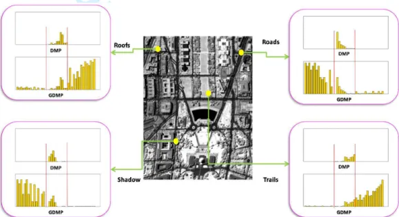
Examples of DMPs and GDMPs for several typical information classes are shown in Fig. 3, where the striking difference between DMPs and GDMPs can be observed. Notably, from Fig. 3, it can be also seen that DMPs are the subset of GDMPs, and the latter can provide more discriminative information.

1 2 3 4 5 6 7 8 9 10 11 12 13 14 15 16 17 18 19 20 21 22 23 24 25 26 27 28 29 30 31 32 33 34 35 36 37 38 39 40 41 42 43 44 45 46 47 48 49 50 51 52 53 54 55 56 57 58 59 60

For Review Only

Fig. 2. Demonstrations for (a) MPs, (b) DMPs, and (c) GDMPs.

Fig. 3. Comparison between DMPs and GDMPs for several typical information classes (roofs, roads, trails, and shadow). The same profiles for DMPs and GDMPs are noted. The sizes of disk-shaped SEs used in this test vary from 2 to 12 with an interval of 2 pixels.

B. Partial Reconstruction of GDMPs

When using geodesic reconstruction, the whole objects can be reconstructed if at least one pixel of the object survives the opening or closing. However, MPs with geodesic reconstruction may lead to over-reconstruction, i.e., some objects that disappeared in the MP without reconstruction may remain present in the MP with geodesic reconstruction. As shown in Fig. 4 (a), the small bright roads on the middle left disappear at a certain scale (SE=6), but these roads still exist when the size of SE reaches 6 in Fig. 4(b). To

1 2 3 4 5 6 7 8 9 10 11 12 13 14 15 16 17 18 19 20 21 22 23 24 25 26 27 28 29 30 31 32 33 34 35 36 37 38 39 40 41 42 43 44 45 46 47 48 49 50 51 52 53 54 55 56 57 58 59 60

For Review Only

solve this problem, partial reconstruction [23] was introduced. If a pixel is connected to another pixel that was not removed after opening or closing and the distance between two connected pixels is smaller than a certain value, the pixel is reconstructed. It should be noted that the geodesic distance, which refers to the length of the shortest path between the two pixels that lies entirely within the object, is used to measure the distance between the two connected pixels and determine the amount of reconstruction. As shown in Fig. 4(c), MPs with partial reconstruction overcomes the problem of over-reconstruction while preserving the shape of objects as much as possible.

The GDMPs with partial reconstruction can be similarly expressed using (5) and (6). Their performance will also be evaluated by the data sets in this study.

Fig. 4. Demonstration and comparison between different morphological reconstruction methods by using opening with disk-shaped SEs of increasing sizes. The sizes of SE vary from 2 to 8 with an interval of 2 pixels. The image shown is a subset of the Pavia University image (Fig. 5(b)): Row 1, 2, 3 corresponds to without reconstruction, geodesic reconstruction, and partial reconstruction, respectively.

1 2 3 4 5 6 7 8 9 10 11 12 13 14 15 16 17 18 19 20 21 22 23 24 25 26 27 28 29 30 31 32 33 34 35 36 37 38 39 40 41 42 43 44 45 46 47 48 49 50 51 52 53 54 55 56 57 58 59 60

For Review Only

C. Feature Selection of GDMPs

Since the proposed GDMPs depict the entire differential morphological profiles, they necessarily contain a lot of redundancies in the feature space. Therefore, random forests (RF) are used in this research to select the most relevant features from GDMPs. RF are a combination of bagging classification trees, that have demonstrated an excellent performance in terms of classification accuracies among a variety of machine learning algorithms [20] [21]. Each classification tree of RF is grown using a bootstrapped sample from the original training samples. At each node of the tree, a series ofindependent variables are randomly selected, decreasing the correlation between the trees in the forest. When choosing the best split from the selected variables at each node, the Gini index [27] [28] indicating the impurity with the lowest value is used to select the most important feature. Subsequently, the most important feature is used to split the corresponding node. Let T represent training set and C_i represent a certain information class, Gini index can be written as:

( ( _i, ) / )( ( _j, ) / ) (9) j i f C T T f C T T ≠

∑ ∑

where f(C ,T)/ T_i is the probability that the selected pixel belongs to class C_i.

Each time a tree is grown into a maximally sized tree without pruning or stopping rules, forming a combination of tree classifier, namely, random forest. Since each tree of RF is grown from a bootstrapped sample, in general, about one-third of the observed training samples will not be used when growing a tree. These observations are called “Out-of-Bag” samples, forming a natural test for each tree. Variable

importance is represented by the decrease of accuracy using “Out-of-Bag” observations when permuting the

values of the corresponding variables. Compared with other machine learning algorithms, RF not only has a good performance for classification, but also provides insight regarding the discriminative ability of each attribute, which actually facilitate to understand the performance of GDMPs. In addition, RF can handle high-dimensional feature space with less computation and be insensitive to noise in training samples [29] [30]. 1 2 3 4 5 6 7 8 9 10 11 12 13 14 15 16 17 18 19 20 21 22 23 24 25 26 27 28 29 30 31 32 33 34 35 36 37 38 39 40 41 42 43 44 45 46 47 48 49 50 51 52 53 54 55 56 57 58 59 60

For Review Only

III.EXPERIMENTS

A. Datasets

Experiments are carried out using the four previously mentioned remote sensing data sets, i.e., 1) HYDICE DC Mall, 2) ROSIS Pavia University, 3) AVIRIS Indian pines, and 4) Worldview-2 Hainan. The data sets are discussed in detail below.

1) DC data set was collected by hyperspectral digital-imagery collection experiment (HYDICE) sensor in August 1995 over the Washington, DC Mall. This data set originally contained 210 bands within the range of wavelength between 0.4-2.4 µm. Noisy channels due to water absorption were removed, resulting in 191

spectral channels available. The main characteristic of DC data set is that it covers an urban area, showing high resolution in both spectral and spatial domains (191 spectral bands with 2.5-m spatial resolution). Spectral characteristics for the same information class are complex (e.g., roofs in the scene are constructed by different materials). However, spectral characteristics of different land cover classes (trees-grass, roofs-trails-roads, water-shadow) are similar due to their overlapped spectral reflectance, making the classification a challenging task. As shown in Fig. 5 (a), this image consists of 1280×307 pixels, with 19,332 pixels labeled as a reference for algorithm verification (Table I).

2) The second data set was acquired over the Engineering School at the University of Pavia by the Reflective Optics System Imaging Spectrometer (ROSIS) sensor. This data set originally contained 115 spectral bands with wavelength ranging from 0.43 to 0.86 µm, with 1.3-m spatial resolution. Some noisy

channels have been removed, resulting in 103 spectral bands. This data set also shows an urban landscape, with nine classes of interest. The challenges for this data set refer to: 1) discrimination between trees, meadows, and soil, and 2) discrimination between asphalt, roofs made of different materials (e.g., bitumen, bricks), as the spectral reflectance of these land cover classes are quite similar. As shown in Fig. 5 (b), this image consists of 610×340 pixels, with 42,776 labeled pixels for model validation (Table II).

3) The third data set was captured over North-Western Indiana by the Airborne Visible/infrared Imaging

1 2 3 4 5 6 7 8 9 10 11 12 13 14 15 16 17 18 19 20 21 22 23 24 25 26 27 28 29 30 31 32 33 34 35 36 37 38 39 40 41 42 43 44 45 46 47 48 49 50 51 52 53 54 55 56 57 58 59 60

For Review Only

Spectrometer (AVIRIS) sensor. This data set consists of 220 spectral bands with a wavelength range from 0.4 to 2.5 µm. The spatial resolution of this data set is 20 m/pixel. This image covers an agriculture area, and

the relative low resolution makes the classification difficult due to the presence of highly mixed pixels. In addition, the number of pixels in the reference data for different information classes is significantly different, which also makes the classification more complicated [30]. As shown in Fig. 5(c), this image consists of 145×145 pixels, with 10,171 labeled pixels for model validation (Table III).

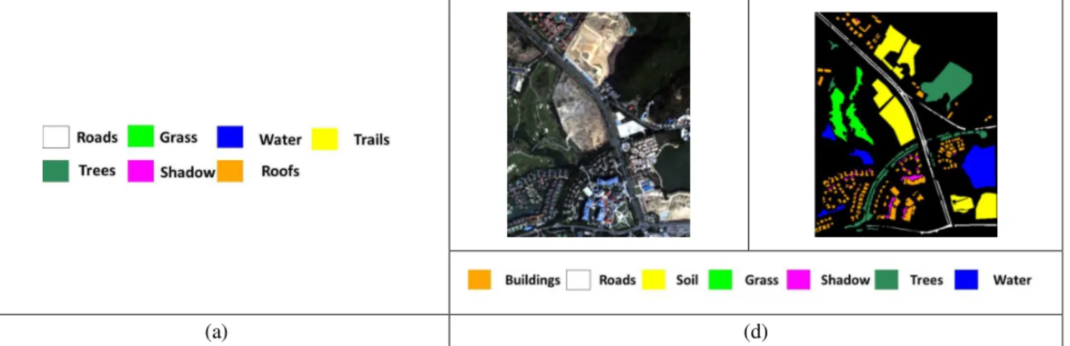
4) The last data set is WorldView-2 high spatial resolution (HSR) data with a 2 m spatial resolution and 8 multispectral bands, over a suburban area in the Hainan province of China. As shown in Fig.5 (d), this image consists of 600×520 pixels, with 31,399 labeled pixels for testing different algorithms (Table IV).

(b) (c) 1 2 3 4 5 6 7 8 9 10 11 12 13 14 15 16 17 18 19 20 21 22 23 24 25 26 27 28 29 30 31 32 33 34 35 36 37 38 39 40 41 42 43 44 45 46 47 48 49 50 51 52 53 54 55 56 57 58 59 60

For Review Only

Fig. 5. Test data sets and their reference maps: (a) HYDICE DC Mall, (b) ROSIS Pavia University, (c) AVIRIS Indian pines, and (d) Worldview-2 Hainan.

TABLE I

NUMBER OF TRAINING AND TEST SAMPLES (HYDICE DC MALL) Information Classes No. of Test Samples Roads 3,334 Grass 3,075 Water 2,882 Trails 1,034 Trees 2,047 Shadow 1,093 Roofs 5,867 Total 19,332 TABLE II

NUMBER OF TRAINING AND TEST SAMPLES (Pavia University) Information Classes No. of Test Samples Asphalt 6,631 Meadows 18,649 Gravel 2,099 Trees 3,064 Metal sheets 1,345 Bare soil 5,029 Bitumen 1,330 Bricks 3,682 Shadow 947 Total 42,776 (a) (d) 1 2 3 4 5 6 7 8 9 10 11 12 13 14 15 16 17 18 19 20 21 22 23 24 25 26 27 28 29 30 31 32 33 34 35 36 37 38 39 40 41 42 43 44 45 46 47 48 49 50 51 52 53 54 55 56 57 58 59 60

For Review Only

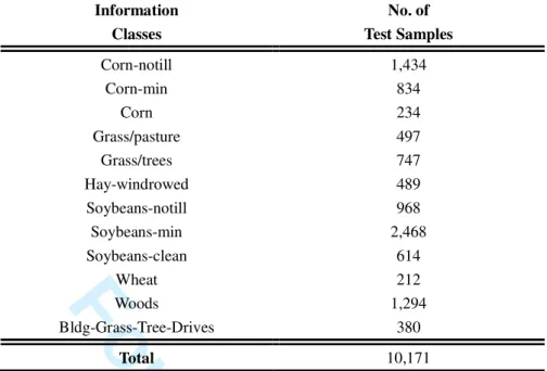
TABLE III

NUMBER OF TRAINING AND TEST SAMPLES (Indian Pines) Information Classes No. of Test Samples Corn-notill 1,434 Corn-min 834 Corn 234 Grass/pasture 497 Grass/trees 747 Hay-windrowed 489 Soybeans-notill 968 Soybeans-min 2,468 Soybeans-clean 614 Wheat 212 Woods 1,294 Bldg-Grass-Tree-Drives 380 Total 10,171 TABLE IV

NUMBER OF TRAINING AND TEST SAMPLES (WorldView-2 Hainan) Information Classes No. of Test Samples Buildings 11,578 Roads 5,357 Soil 22,189 Grass 7,417 Shadow 1,427 Trees 14,086 Water 11,209 Total 73,263 B. Experimental Setup

The parameter settings in the experiments are listed below.

1) Morphological profiles: Disk-shaped SEs ranging from 2 to 12 are used to obtain DMPs and GDMPs on the first three principal components (PCs) of original image with geodesic reconstruction and partial reconstruction, respectively.

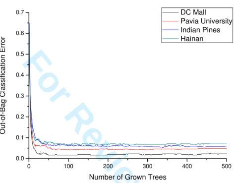
2) Classifier: RF is used for feature selection and classification with 200 decision trees, by considering both accuracy and efficiency (analyzed in Fig.6).

3) Accuracy assessment: Overall accuracy (OA), average accuracy (AA), and kappa coefficient (Kappa)

1 2 3 4 5 6 7 8 9 10 11 12 13 14 15 16 17 18 19 20 21 22 23 24 25 26 27 28 29 30 31 32 33 34 35 36 37 38 39 40 41 42 43 44 45 46 47 48 49 50 51 52 53 54 55 56 57 58 59 60

For Review Only

computed from the confusion matrix are used to evaluate the classification accuracies.

4) Training: 50 samples per class selected from the reference map are used to train the RF model. The experiments are repeated ten times with different starting training samples and the average accuracies are reported.

Fig. 6. Relationship between “out-of-bag” classification error and the number of decision trees of random forest. It can be observed that after 100~200 trees used in the forest, classification accuracies become steady.

C. Experimental results with geodesic reconstruction

Test 1: The class-specific accuracies of the HYDICE DC MALL based on classification of DMPs and

GDMPs are presented in Table V. The classification maps of DMPs and GDMPs are shown in Fig.7. In this data set, the raw spectral-based classification has difficulty in discriminating between roofs, roads and trails. The classification accuracies can be improved by introducing DMPs and GDMPs. Specifically, compared to the raw classification, the improvements of OA achieved by using DMPs and GDMPs are 0.7% and 4.7%, respectively. For a visual comparison, compared to raw spectral-based classification, the accuracy improvements achieved by DMPs and GDMPs for each class are shown in Fig. 11(a). It can be seen that GDMPs outperform DMPs in terms of the accuracy scores. In particular, GDMPs can improve the

0 100 200 300 400 500 0.0 0.1 0.2 0.3 0.4 0.5 0.6 0.7 O u t-o f-B a g C la s s if ic a ti o n E rr o r

Number of Grown Trees

DC Mall Pavia University Indian Pines Hainan 1 2 3 4 5 6 7 8 9 10 11 12 13 14 15 16 17 18 19 20 21 22 23 24 25 26 27 28 29 30 31 32 33 34 35 36 37 38 39 40 41 42 43 44 45 46 47 48 49 50 51 52 53 54 55 56 57 58 59 60

For Review Only

accuracies of roofs significantly (from 81% to 93%), which can be attributed to exploitation of the entire shape spectrum considered in the GDMPs.

TABLE V

Accuracies (%) for DMPs and GDMPs with geodesic reconstruction for the DC Mall image Feature Classes RAW DMPs GDMPs Roads 97.97 97.88 98.00 Grass 99.54 99.84 100.00 Water 99.51 99.72 100.00 Trails 95.38 97.05 98.82 Trees 98.42 98.42 98.67 Shadow 98.26 98.63 98.90 Roofs 79.28 81.05 93.44 OA = 92.73 AA = 95.48 Kappa = 91.18 OA = 93.43 AA= 96.08 Kappa = 92.03 OA = 97.41 AA = 98.26 Kappa = 96.82 (a) (b) (c)

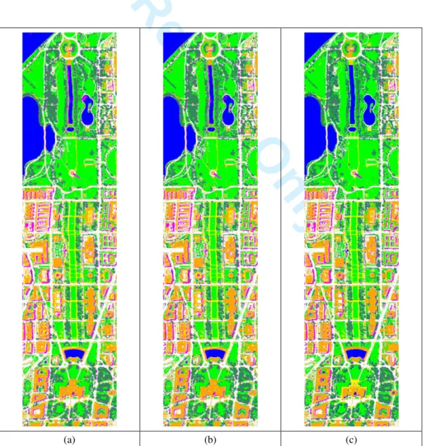
Fig. 7. RF classification maps for the DC Mall image: (a) The raw hyperspectral image, (b) DMPs, and (c) GDMPs. 1 2 3 4 5 6 7 8 9 10 11 12 13 14 15 16 17 18 19 20 21 22 23 24 25 26 27 28 29 30 31 32 33 34 35 36 37 38 39 40 41 42 43 44 45 46 47 48 49 50 51 52 53 54 55 56 57 58 59 60

For Review Only

Test 2: The class-specific accuracies of the Pavia University in classification based on the DMPs and

GDMPs are presented in Table VI. The classification maps based on DMPs and GDMPs are shown in Fig. 8. Similarly as in Test 1, DMPs and GDMPs can obtain satisfactory results, compared with spectral-based

classification (OA is substantially increased from 73.85% to 86.62% and 96.22%, respectively). It can also be seen that the GDMPs surpass DMPs on the classification accuracies significantly as the former considers the entire morphological profiles. In this experiment, the improvements for the class-specific accuracies compared to the raw spectral-based classification are shown in Fig. 11(b). It can be seen that the use of DMPs and GDMPs provides higher accuracies for all the classes. In particular, the increments of the accuracies achieved by the proposed GDMPs are much higher than with the traditional DMPs, especially for the classes meadows, gravel, bare soil, and bricks.

TABLE VI

Accuracies (%) for DMPs and GDMPs with geodesic reconstruction for the Pavia University image. Feature Classes RAW DMPs GDMPs Asphalt 72.22 96.52 98.36 Meadows 67.92 77.39 95.10 Gravel 65.22 89.14 96.24 Trees 86.65 95.43 95.82 Metal sheets 98.74 99.11 98.88 Bare soil 76.38 89.14 94.55 Bitumen 89.70 98.05 94.51 Bricks 76.15 85.12 97.18 Shadow 100.00 100.00 100.00 OA = 73.85 AA = 81.44 Kappa = 67.03 OA = 86.62 AA= 92.18 Kappa = 82.87 OA = 96.22 AA = 96.98 Kappa = 95.28 1 2 3 4 5 6 7 8 9 10 11 12 13 14 15 16 17 18 19 20 21 22 23 24 25 26 27 28 29 30 31 32 33 34 35 36 37 38 39 40 41 42 43 44 45 46 47 48 49 50 51 52 53 54 55 56 57 58 59 60

For Review Only

(a) (b) (c)

Fig. 8. Classification maps for the Pavia University image: (a) The raw hyperspectral image, (b) DMPs, and (c) GDMPs.

Test 3: The class-specific accuracies of the Indian Pines image achieved by using the DMPs and GDMPs

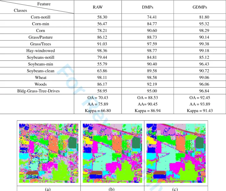
are presented in Table VII. The classification maps for DMPs and GDMPs are compared in Fig. 9 for a visual inspection. For this data set, the original spectral-based classification has difficulty in correctly classifying the 12 information classes, resulting in a relatively low overall accuracy (70.43%). However, the OA is significantly raised to 88.53% and 92.45%, respectively, by employing DMPs and GDMPs. The accuracy increment for each class is demonstrated in Fig. 11(c), where a similar phenomenon is observed, i.e., GDMPs are superior to DMPs interms of classification accuracies for most information classes. Please note that this test image is related to an agricultural area, which shows that the proposed GDMPs are not only effective in urban area but also in agricultural areas.

1 2 3 4 5 6 7 8 9 10 11 12 13 14 15 16 17 18 19 20 21 22 23 24 25 26 27 28 29 30 31 32 33 34 35 36 37 38 39 40 41 42 43 44 45 46 47 48 49 50 51 52 53 54 55 56 57 58 59 60

For Review Only

TABLE VII

Accuracies (%) for DMPs and GDMPs with geodesic reconstruction for the Indian Pines image Feature Classes RAW DMPs GDMPs Corn-notill 58.30 74.41 81.80 Corn-min 56.47 84.77 95.32 Corn 78.21 90.60 98.29 Grass/Pasture 86.12 88.73 90.14 Grass/Trees 91.03 97.59 99.38 Hay-windrowed 98.36 98.77 99.18 Soybeans-notill 79.44 84.81 85.12 Soybeans-min 55.79 90.40 96.43 Soybeans-clean 63.86 89.58 90.72 Wheat 98.11 98.58 99.06 Woods 86.17 92.19 96.06 Bldg-Grass-Tree-Drives 58.95 95.00 96.84 OA = 70.43 AA = 75.89 Kappa = 66.80 OA = 88.53 AA= 90.45 Kappa = 86.94 OA = 92.45 AA = 93.89 Kappa = 91.43 (a) (b) (c)

Fig. 9. Classification maps for the Indian Pines image: (a) The raw hyperspectral image, (b) DMPs, and (c) GDMPs.

Test 4: The class-specific accuracies of the WorldView-2 Hainan image achieved by using DMPs and

GDMPs are provided in Table VIII. Furthermore, their classification maps shown in Fig. 10. For this data set, the OA of the initial spectral-only classification is 87.08%, subject to the misclassifications between buildings, roads, and soil. The incorporation of the spatial information can increase the accuracy (OA) by 7.23% and 9.51% for DMPs and GDMPs, respectively. For the improvements of the class-specific accuracy compared to the spectral-based classification [Fig. 11(d)], it can be observed that once again GDMPs provide better results for all the information classes than the traditional DMPs, especially for the buildings

1 2 3 4 5 6 7 8 9 10 11 12 13 14 15 16 17 18 19 20 21 22 23 24 25 26 27 28 29 30 31 32 33 34 35 36 37 38 39 40 41 42 43 44 45 46 47 48 49 50 51 52 53 54 55 56 57 58 59 60

For Review Only

(86.04% for the DMPs and 92.82% for the GDMPs), as the proposed GDMPs can describe the structural features in a more appropriate manner.

TABLE VIII

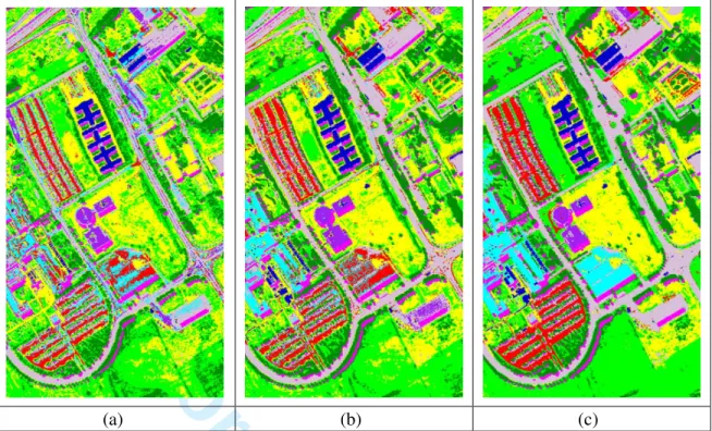
Accuracies (%) of DMPs and GDMPs with geodesic reconstruction for the Hainan image Feature Classes RAW DMPs GDMPs Buildings 58.31 86.04 92.82 Roads 84.60 93.84 96.98 Soil 91.06 98.10 98.74 Grass 96.85 98.10 98.76 Shadow 91.10 92.29 94.86 Trees 89.73 92.30 92.84 Water 99.80 99.80 99.90 OA = 87.08 AA = 87.35 Kappa = 84.07 OA = 94.31 AA= 94.14 Kappa = 93.28 OA = 96.59 AA = 96.41 Kappa = 95.98 (a) (b) (c)

Fig. 10. RF classification maps for the Hainan image: (a) The raw hyperspectral image, (b) DMPs, and (c) GDMPs. 1 2 3 4 5 6 7 8 9 10 11 12 13 14 15 16 17 18 19 20 21 22 23 24 25 26 27 28 29 30 31 32 33 34 35 36 37 38 39 40 41 42 43 44 45 46 47 48 49 50 51 52 53 54 55 56 57 58 59 60

For Review Only

(a) Test 1 (b)Test 2 Roa ds Gra ss Wat er Trai ls Tree s Shad ow Roo fs 0 5 10 15 DMPs GDMPs Asph alt Mea dow s Gra vel Tree s Met al s heet s Bare soi l Bitu men _Bricks Shad ow 0 5 10 15 20 25 30 DMPs GDMPs 1 2 3 4 5 6 7 8 9 10 11 12 13 14 15 16 17 18 19 20 21 22 23 24 25 26 27 28 29 30 31 32 33 34 35 36 37 38 39 40 41 42 43 44 45 46 47 48 49 50 51 52 53 54 55 56 57 58 59 60

For Review Only

(c) Test 3

(d)Test 4

Fig. 11. Percentage of accuracy improvements of each class by the DMPs/GDMPs (geodesic reconstruction) compared to the raw spectral-based method in (a) DC image, (b) Pavia University, (c) Indian Pines, and (d) Hainan.

D. Experiment results with partial reconstruction

Corn -not ill Corn -min Corn Gras s/Pas ture Gras s/Tre es Ha y-wind rowe d Soyb eans -not ill Soyb eans -min Soyb eans -clea n Whe at Woo ds Bldg -Gra ss-T re e-Drive s 0 5 10 15 20 25 30 35 40 DMPs GDMPs Build ings Roa ds _Soil Gra ss Shad ow Tree s Wat er 0 5 10 15 20 25 30 35 DMPs GDMPs 1 2 3 4 5 6 7 8 9 10 11 12 13 14 15 16 17 18 19 20 21 22 23 24 25 26 27 28 29 30 31 32 33 34 35 36 37 38 39 40 41 42 43 44 45 46 47 48 49 50 51 52 53 54 55 56 57 58 59 60

For Review Only

TABLE IX

Comparison of overall accuracy (%) achieved by spectral bands, DMPs and GDMPs with partial reconstruction. Features

Datasets RAW DMPs-Partial GDMPs-Partial

DC Mall 92.73 93.85 96.54

Pavia University 73.85 86.16 90.26

Indian Pines 70.43 87.96 91.08

Hainan 87.08 94.94 96.24

Next, a comparative analysis for DMPs and GDMPs, by partial reconstruction (DMPs-Partial, GDMPs-Partial)，respectively, was conducted. The results are given in TABLE IX. From the results, it can be observed that GDMPs-Partial outperforms the DMPs-Partial in all the test data sets. Specifically, compared to the classification accuracy of DMPs-Partial, the improvements for GDMPs-Partial in OA are about 2.69%, 4.10%, 3.12% and 1.3% for the DC Mall, Pavia University, Indian Pines, and Hainan data sets, respectively. It is shown that the proposed GDMPs can also provide more accurate classification result under the circumstance of the morphological partial reconstruction.

E. Feature Analysis

In order to analyze the information redundancy of GDMPs and investigate the relationship between classification accuracy (overall accuracy) and dimensionality of the feature space, feature selection was conducted according to feature importance quantified by random forest “Out-of-Bag” error. Fig. 12 shows

the relationship between classification accuracy and the dimensionality of the feature space which simultaneously consists of hyperspectral space and GDMPs (geodesic reconstruction). It can be found that curves become stable when dimensionalities of a feature reach a certain number and the turning points of the accuracy curves after which the trend becomes stable are 11, 13, 41 and 45, corresponding to DC Mall, Pavia University, Indian Pines, and Hainan, respectively.

Moreover, a detailed analysis on the source of selected features was conducted:

1) DC Mall: The turning point corresponds to 11 features, which can obtain similar classification accuracy with the full feature space [Fig. 13(a)]. Among these 11 selected features, 10 features are derived from GDMPs, and all the 10 features are from the across-scale morphological profiles that cannot be obtained by

1 2 3 4 5 6 7 8 9 10 11 12 13 14 15 16 17 18 19 20 21 22 23 24 25 26 27 28 29 30 31 32 33 34 35 36 37 38 39 40 41 42 43 44 45 46 47 48 49 50 51 52 53 54 55 56 57 58 59 60

For Review Only

the traditional DMPs.

2) Pavia University: In this test, according to the accuracy curve [Fig. 13(b)], 12 of 13 selected features are from the across-scale differential morphological profiles (GDMPs).

3) Indian Pines: In this case, the first 41 features are selected and analyzed since they can achieve similar classification accuracy with the full feature space [Fig. 13(c)]. However, only 2 of the 41 selected features come from original spectral data, and the remaining 39 features are generated by GDMPs. Please note that 32 of these 39 GDMPs refer to the across-scale morphological profiles, but only 7 features refer to the traditional DMPs.

4) Hainan: In this test, a total of 45 features are selected and focused on [Fig. 13(d)]. 36 of the 45 selected features are derived from GDMPs, and 32 of the 36 features correspond to the across-scale profiles.

The feature contributions are analyzed in Figs. 12 and 13. The importance of the GDMPs features as well as the spectral signals is computed and ranked based on the Gini index in the RF decision. The number of each feature sources (spectral, DMPs, GDMPs) that are selected at the turning point, first 20-D, and first 50-D is recorded for comparison. Please note that the turning point (Fig. 13) indicates where the selected features can achieve a steady classification accuracy that is comparable to the full feature space.

(a) 1 2 3 4 5 6 7 8 9 10 11 12 13 14 15 16 17 18 19 20 21 22 23 24 25 26 27 28 29 30 31 32 33 34 35 36 37 38 39 40 41 42 43 44 45 46 47 48 49 50 51 52 53 54 55 56 57 58 59 60

For Review Only

_(b)

(c)

Fig. 12. Feature importance analysis at: (a) the turning point, (b) first 20-D, and (c) first 50-D in the hybrid feature space selected.

According to the above analysis, we can draw the conclusion that the relevant features from GDMPs play a much more important role than DMPs and spectral signals in the classification task, as they are dominant in the selected feature space in all the test cases. Compared to original DMPs, across-scale differential morphological profiles make it possible to obtain the entire differential profiles, depicting the full shape spectrum of objects in an image. In addition, through feature selection procedure implemented by RF, a similar classification accuracy can be reached with much less features compared to the high-dimensional hyperspectral and GDMPs feature space.

1 2 3 4 5 6 7 8 9 10 11 12 13 14 15 16 17 18 19 20 21 22 23 24 25 26 27 28 29 30 31 32 33 34 35 36 37 38 39 40 41 42 43 44 45 46 47 48 49 50 51 52 53 54 55 56 57 58 59 60

For Review Only

(a) (b)

(c) (d)

Fig. 13. Relationship between classification accuracy (overall accuracy) and the dimensionality of feature space consisting of spectral bands and GDMPs. The so-called turning points (from which accuracy tends to be stable and comparable to the full feature space) are marker in the accuracy curves.

F. Influence of the Number of Training Samples

The classification accuracies as a function of the number of training samples are demonstrated in Fig. 14. Specifically, four groups of training samples are used for investigating the influence of the number of training samples on the classification accuracies: 25, 50, 75, and 100 pixels per class. From the results, it can be observed that in all the experiments, the proposed GDMPs (both geodesic and partial reconstruction) can achieve higher accuracies than DMPs regardless of the number of training samples.

1 2 3 4 5 6 7 8 9 10 11 12 13 14 15 16 17 18 19 20 21 22 23 24 25 26 27 28 29 30 31 32 33 34 35 36 37 38 39 40 41 42 43 44 45 46 47 48 49 50 51 52 53 54 55 56 57 58 59 60

For Review Only

(a) DC Mall (b) Pavia Univeristy (c) Indian Pines 1 2 3 4 5 6 7 8 9 10 11 12 13 14 15 16 17 18 19 20 21 22 23 24 25 26 27 28 29 30 31 32 33 34 35 36 37 38 39 40 41 42 43 44 45 46 47 48 49 50 51 52 53 54 55 56 57 58 59 60

For Review Only

Fig. 14. Classification accuracies with different training sample sizes, for (a) DC Mall, (b) Pavia University, (c) Indian Pines, and (d) Hainan.

IV.CONCLUSION

In this study, we propose generalized differential morphological profiles (GDMPs) for spatial/structural feature extraction and classification of remote sensing images. Compared to the traditional DMPs, the main superiority of GDMPs is that they can describe across-scale differential morphological profiles, which is

more appropriate for the multiscale characteristics and complex landscapes of remote sensing image scenes. Subsequently, in order to address the information redundancy in the GDMPs, random forest is used for feature selection and classification.

In this research, the important conclusions drawn from the experimental results are summarized as follows:

DMPs and GDMPs can greatly improve the classification results, when compared to spectral-only information, since DMPs and GDMPs can effectively represent the structural information of an image for discriminating between spectrally similar classes.

The proposed GDMPs show a better performance in terms of classification accuracy than the original DMPs under circumstances of both geodesic and partial reconstruction. It can be attributed to the ability of the GDMPs to provide scale-span differential profiles, some of which are more informative for the complex geospatial space and more discriminative for the spectral-alike information classes.

(d) Hainan 1 2 3 4 5 6 7 8 9 10 11 12 13 14 15 16 17 18 19 20 21 22 23 24 25 26 27 28 29 30 31 32 33 34 35 36 37 38 39 40 41 42 43 44 45 46 47 48 49 50 51 52 53 54 55 56 57 58 59 60

For Review Only

RF is used to interpret the GDMPs as it is capable of dealing with high-dimension data with redundant information and evaluating the variable importance according to its “Out-of-Bag” error. It

should be noted that only a few features selected according to feature importance can achieve considerable accuracy of the original feature space.

In summary, it can be concluded that the newly introduced GDMPs can describe more complete structural information of an image and can be a standard technique for feature extraction from remote sensing images. In the future, we plan to discuss the different methods of dimension reduction implemented for the proposed GDMPs and attempt more applications based on GDMPs, such as change detection, object detection.

ACKNOWLEDGMENT

The authors would like to thank Prof. D. A. Landgrebe, Purdue University, USA, for providing the HYDICE dataset and Prof. P. Gamba, University of Pavia, Italy, for providing the Pavia University data.

References

[1] S. W. Myint, N. Lam, and J. M. Tyler, Wavelets for Urban Spatial Feature Discrimination: Comparisons with Fractal,

Spatial Autocorrelation, and Spatial Co-occurrence Approaches, 2004.

[2] X. Huang, L. P. Zhang, and P. X. Li, “An adaptive multiscale information fusion approach for feature extraction and classification of IKONOS multispectral imagery over urban areas,” Ieee Geoscience And Remote Sensing Letters, vol. 4, no. 4, pp. 654-658, Oct, 2007.

[3] M. Pesaresi, A. Gerhardinger, and F. Kayitakire, “A Robust Built-Up Area Presence Index by Anisotropic Rotation-Invariant Textural Measure,” Ieee Journal Of Selected Topics In Applied Earth Observations And Remote Sensing,

vol. 1, no. 3, pp. 180-192, Sep, 2008.

[4] X. Huang, X. B. Liu, and L. P. Zhang, “A Multichannel Gray Level Co-Occurrence Matrix for Multi/Hyperspectral Image Texture Representation,” Remote Sensing, vol. 6, no. 9, pp. 8424-8445, Sep, 2014.

[5] S. Geman, and D. Geman, “Stochastic relaxation, gibbs distributions, and the bayesian restoration of images,” IEEE Trans

Pattern Anal Mach Intell, vol. 6, no. 6, pp. 721-41, Jun, 1984.

[6] C. Zhu, and X. Yang, “Study of remote sensing image texture analysis and classification using wavelet,” International

Journal of Remote Sensing, vol. 19, no. 16, pp. 3197-3203, 1998/01/01, 1998.

[7] X. Huang, and L. P. Zhang, “An SVM Ensemble Approach Combining Spectral, Structural, and Semantic Features for the Classification of High-Resolution Remotely Sensed Imagery,” Ieee Transactions on Geoscience And Remote Sensing, vol. 51, no. 1, pp. 257-272, Jan, 2013.

[8] W. Xiaoyu, T. X. Han, and Y. Shuicheng, "An HOG-LBP human detector with partial occlusion handling." pp. 32-39. [9] C. Song, F. Yang, and P. Li, "Rotation invariant texture measured by local binary pattern for remote sensing image

classification." pp. 3-6.

[10] M. Pesaresi, and J. A. Benediktsson, “A new approach for the morphological segmentation of high-resolution satellite

1 2 3 4 5 6 7 8 9 10 11 12 13 14 15 16 17 18 19 20 21 22 23 24 25 26 27 28 29 30 31 32 33 34 35 36 37 38 39 40 41 42 43 44 45 46 47 48 49 50 51 52 53 54 55 56 57 58 59 60

For Review Only

imagery,” Ieee Transactions on Geoscience And Remote Sensing, vol. 39, no. 2, pp. 309-320, Feb, 2001.

[11] J. A. Benediktsson, M. Pesaresi, and K. Arnason, “Classification and feature extraction for remote sensing images from urban areas based on morphological transformations,” Ieee Transactions on Geoscience And Remote Sensing, vol. 41, no. 9, pp. 1940-1949, Sep, 2003.

[12] J. Chanussot, J. A. Benediktsson, and M. Fauvel, “Classification of remote sensing images from urban areas using a fuzzy possibilistic model,” Ieee Geoscience And Remote Sensing Letters, vol. 3, no. 1, pp. 40-44, Jan, 2006.

[13] X. Huang, L. P. Zhang, and L. Wang, “Evaluation of Morphological Texture Features for Mangrove Forest Mapping and Species Discrimination Using Multispectral IKONOS Imagery,” IEEE Geoscience and Remote Sensing Letters, vol. 6, no. 3, pp. 393-397, 2009.

[14] J. A. Benediktsson, J. A. Palmason, and J. R. Sveinsson, “Classification of hyperspectral data from urban areas based on extended morphological profiles,” IEEE Transactions on Geoscience and Remote Sensing, vol. 43, no. 3, pp. 480-491, 2005.

[15] M. Dalla Mura, J. A. Benediktsson, B. Waske, and L. Bruzzone, “Morphological attribute profiles for the analysis of very high resolution images,” Geoscience and Remote Sensing, IEEE Transactions on, vol. 48, no. 10, pp. 3747-3762, 2010. [16] M. D. Mura, A. Villa, J. A. Benediktsson, J. Chanussot, and L. Bruzzone, “Classification of hyperspectral images by using

extended morphological attribute profiles and independent component analysis,” Geoscience and Remote Sensing

Letters, IEEE, vol. 8, no. 3, pp. 542-546, 2011.

[17] P. R. Marpu, M. Pedergnana, M. D. Mura, S. Peeters, J. A. Benediktsson, and L. Bruzzone, “Classification of hyperspectral data using extended attribute profiles based on supervised and unsupervised feature extraction techniques,”

International Journal of Image and Data Fusion, vol. 3, no. 3, pp. 269-298, 2012.

[18] X. Huang, X. H. Guan, J. A. Benediktsson, L. P. Zhang, J. Li, A. Plaza, and M. Dalla Mura, “Multiple Morphological Profiles From Multicomponent-Base Images for Hyperspectral Image Classification,” Ieee Journal Of Selected Topics In Applied

Earth Observations And Remote Sensing, vol. 7, no. 12, pp. 4653-4669, Dec, 2014.

[19] P. Ghamisi, M. Dalla Mura, and J. A. Benediktsson, “A survey on spectral–spatial classification techniques based on attribute profiles,” Geoscience and Remote Sensing, IEEE Transactions on, vol. 53, no. 5, pp. 2335-2353, 2015.

[20] L. Breiman, “Random forests,” Machine Learning, vol. 45, no. 1, pp. 5-32, Oct, 2001.

[21] T. Bylander, “Estimating generalization error on two-class datasets using out-of-bag estimates,” Machine Learning, vol. 48, no. 1-3, pp. 287-297, Jul-Sep, 2002.

[22] J. Serra, Image Analysis and Mathematical Morphology: Academic Press, Inc., 1983.

[23] R. Bellens, S. Gautama, L. Martinez-Fonte, W. Philips, J. C.-W. Chan, and F. Canters, “Improved Classification of VHR Images of Urban Areas Using Directional Morphological Profiles,” IEEE Transactions on Geoscience and Remote Sensing,

vol. 46, no. 10, pp. 2803-2813, 2008.

[24] W. Z. Liao, R. Bellens, A. Pizurica, W. Philips, and Y. G. Pi, “Classification of Hyperspectral Data Over Urban Areas Using Directional Morphological Profiles and Semi-Supervised Feature Extraction,” Ieee Journal Of Selected Topics In Applied

Earth Observations And Remote Sensing, vol. 5, no. 4, pp. 1177-1190, Aug, 2012.

[25] P. Soille, Morphological image analysis: principles and applications: Springer Science & Business Media, 2013.

[26] M. Fauvel, J. A. Benediktsson, J. Chanussot, and J. R. Sveinsson, “Spectral and Spatial Classification of Hyperspectral Data Using SVMs and Morphological Profiles,” Ieee Transactions on Geoscience And Remote Sensing, vol. 46, no. 11, pp. 3804-3814, Nov, 2008.

[27] L. Breiman, J. Friedman, C. J. Stone, and R. A. Olshen, Classification and regression trees: CRC press, 1984.

[28] M. Pal, “Random forest classifier for remote sensing classification,” International Journal of Remote Sensing, vol. 26, no. 1, pp. 217-222, 2005.

[29] L. Breiman, "RF/tools: A class of two-eyed algorithms."

[30] P. Ghamisi, J. A. Benediktsson, G. Cavallaro, and A. Plaza, “Automatic Framework for Spectral-Spatial Classification Based on Supervised Feature Extraction and Morphological Attribute Profiles,” IEEE Journal of Selected Topics in Applied Earth

Observations and Remote Sensing, vol. 7, no. 6, pp. 2147-2160, 2014.

1 2 3 4 5 6 7 8 9 10 11 12 13 14 15 16 17 18 19 20 21 22 23 24 25 26 27 28 29 30 31 32 33 34 35 36 37 38 39 40 41 42 43 44 45 46 47 48 49 50 51 52 53 54 55 56 57 58 59 60