A Semi-Supervised Synthetic Aperture
Radar (SAR) Image Recognition Algorithm
Based on an Attention Mechanism and
Bias-Variance Decomposition
FEI GAO 1, WEI SHI 1, JUN WANG1, AMIR HUSSAIN2, AND HUIYU ZHOU3 1School of Electronic and Information Engineering, Beijing University of Aeronautics and Astronautics, Beijing 100191, China 2Cognitive Big Data and Cyber-Informatics Laboratory, School of Computing, Edinburgh Napier University, Edinburgh EH10 5DT, U.K. 3Department of Informatics, The University of Leicester, Leicester LE1 7RH, U.K.
Corresponding author: Jun Wang ([email protected])
This work was supported in part by the National Natural Science Foundation of China under Grant 61771027, Grant 61071139, Grant 61471019, Grant 61501011, and Grant 61171122. The work of A. Hussain was supported in part by the U.K. Engineering and Physical Sciences Research Council (EPSRC) under Grant EP/M026981/1. The work of H. Zhou was supported in part by the U.K. EPSRC under Grant EP/N508664/1, Grant EP/R007187/1, and Grant EP/N011074/1, and in part by the Royal Society-Newton Advanced Fellowship under Grant NA160342.
ABSTRACT Synthetic Aperture Radar (SAR) target recognition is an important research direction of SAR image interpretation. In recent years, most of machine learning methods applied to SAR target recognition are supervised learning which requires a large number of labeled SAR images. However, labeling SAR images is expensive and time-consuming. We hereby propose an end-to-end semi-supervised recognition method based on an attention mechanism and bias-variance decomposition, which focuses on the unlabeled data screening and pseudo-labels assignment. Different from other learning methods, the training set in each iteration is determined by a module that we here propose, called dataset attention module (DAM). Through DAM, the contributing unlabeled data will have more possibilities to be added into the training set, while the non-contributing and hard-to-learn unlabeled data will receive less attention. During the training process, each unlabeled data will be input into the network for prediction. The pseudo-label of the unlabeled data is considered to be the most probable classification in the multiple predictions, which reduces the risk of the single prediction. We calculate the prediction bias-and-variance of all the unlabeled data and use the result as the criteria to screen the unlabeled data in DAM. In this paper, we carry out semi-supervised learning experiments under different unlabeled rates on the Moving and Stationary Target Acquisition and Recognition (MSTAR) dataset. The recognition accuracy of our method is better than several state of the art semi-supervised learning algorithms.
INDEX TERMS Attention mechanism, bias-variance decomposition, SAR target recognition,
semi-supervised learning.
I. INTRODUCTION
SAR has the ability to capture the images of the earth’s surface in nearly all weather conditions from a long dis-tance. Together with its high spatial resolutions, SAR plays a more and more important role at the fields of geosciences, hydrology and bionomics. Synthetic Aperture Radar auto-matic target recognition (SAR-ATR) has been established for
The associate editor coordinating the review of this manuscript and approving it for publication was Nilanjan Dey.
several years. The method of SAR target recognition includes template matching [1], [2], model-based methods [3]–[5] and machine learning [6]–[13]. Template matching needs to store plenty of templates and model-based methods need to deal with the problems in feature extraction. Traditional machine learning methods require complex preprocessing SAR images, including denoising and feature extraction. SAR images are sensitive to the change of target azimuth and orientation, which cause many problems to the tra-ditional SAR target recognition methods. In recent years,
with the development of Convolutional Neural Networks (CNNs) [14], applying CNNs in SAR target recognition has attracted much attention. Chen and Sizhe [6] present an all-convolutional network, which only consists of sparsely connected layers, to alleviate the overfitting problem during training with limited SAR images. In order to distinguish categories more accurately, Tianet al.[7] introduce a class of separability measurement into the cost function and extract SAR image features using an improved CNN.
The features of each layer are obtained from the local regions of the upper layer by convolution kernels, which enable CNNs to learn and represent features bet-ter. To enhance the performance of CNNs, researches have mainly investigated from three important factors of networks: depth [15]–[18], width [19]–[21] and cardinal-ity [22]. Recently, researchers have linked deep learn-ing with human brain perception to improve the network performance [23]–[25]. The latest system combines atten-tion mechanisms with CNNs to increase the representaatten-tion power of CNNs. Attention mechanisms are a key ability for humans to select the regions of interest from a large scene. Human obtains the focus of attention by scanning the global image quickly, and then investing more attention resources onto the target whilst reducing useless informa-tion. Attention mechanisms greatly improve efficiency and accuracy of visual information processing. Wanget al.[26] propose Residual Attention Network, which combines the deep convolution neural networks (DCNNs) and an attention mechanism. The network achieves high recognition accu-racy by refining the feature maps. Squeeze-and-Excitation Networks (SENets) [27] boost the representation ability of CNNs by adaptively recalibrating channel-wise feature responses. In the Squeeze-and-Excitation block, they used global average-pooled features to compute channel-wise attention. Woo et al. [28] propose a Convolutional Block Attention Module (CBAM) which refines the feature maps from two separate dimensions: channel and spatial. Because CBAM is a lightweight and general module, it can be inte-grated into most of the CNN architectures.
However, the above-mentioned CNNs need vast amounts of labeled data to achieve high recognition accuracy. For SAR images, labeling is expensive and time-consuming. Semi-supervised learning combines supervised learn-ing with unsupervised learnlearn-ing, which can effectively reduce their dependence on the labeled samples. Tradi-tional semi-supervised methods include generative meth-ods [29], [30], semi-supervised SVM [31], [32], graph semi-supervised learning [33], [34], disagreement-based method [35] and semi-supervised clustering [36], [37]. Most of the current semi-supervised learning algorithms focus on generating pseudo-labels for unlabeled data and using them together with labeled data from the start of the network training. These algorithms haven’t taken into account that the unlabeled set may have some hard-to-learn and redundant data which need to be filtered out before using them.
In this paper, we intend to achieve two goals in semi-supervised methods: one is to improve the security of the pseudo-labels assignment and the other one is to use less training data to maintain the prediction accuracy by screening the unlabeled data. In order to reduce the risk of single prediction, the pseudo-labels are assigned by the statistical results of multiple predictions. In our method, a baseline model is trained using the labeled dataset firstly. When the training process becomes stable, we use the network to pre-dict the unlabeled data after each iteration and record the prediction probability corresponding to each classification. The pseudo-label of the unlabeled data is considered to be the classification with the highest average prediction probability among multiple predictions. To achieve the second target, we combine an attention mechanism and semi-supervised learning, and propose a new attention module called dataset attention module (DAM). Before inputting the unlabeled data into DAM, we group them into several sub-datasets. Group screening will reduce the parameters of DAM. We define a set of Dataset Screening Factors (DSFs) to adjust the attention on individual sub-datasets, where each sub-dataset corresponds to one DSF. DSFs determine how much data in each sub-dataset will be added to the training set to the current iteration. Through the continuous network training, the focus of the attention of DAM will be more accurate. DAM will invest more attention resources on the unlabeled samples that can boost the performance of the network. The detailed process of grouping the unlabeled data can be described as follows: For each unlabeled sample, we calculate the sum of its prediction bias-and-variance, and then sort them according to the ascending order of the sum. After reordering these samples, we divide them into several sub-datasets at the same size. The number of the sub-datasets is a hyper-parameter, which varies according to the amount of the training data.
The training process of the baseline model and DAM is different. We use a cross entropy loss function to update the parameters in the baseline model. When DAM is integrated with the baseline model, the updating of DSFs is achieved after each iteration, while the other network parameters are updated after each batch in one iteration. The reason why DSFs aren’t updated together with the other parameters is to ensure that the same DSFs are used in the current iteration. So, in one iteration, the training set will stay unchanged. The screening of the unlabeled data and the assignment of the pseudo-labels are conducted by the network itself, without human participation. The main contributions made in this paper are follows:
Firstly, we propose a new attention mechanism by combin-ing the attention mechanism and semi-supervised learncombin-ing, namely DAM. Through DAM, the unlabeled data is screened to eliminate the non-contributing and redundant data. The model learns more accurate knowledge and improves SAR target recognition accuracy.
Secondly, in our method, the assignment of pseudo-labels is done by statistical results of multiple predictions, which
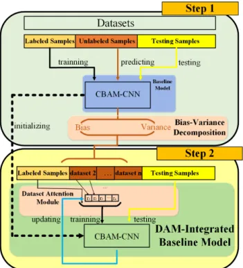
FIGURE 1. Framework of the proposed method.
reduces the contingency of single prediction and improves the correctness of pseudo-labels.
Finally, the proposed semi-supervised learning algorithm adopts end-to-end learning and can maintain good recogni-tion accuracy in different noisy environments.
The rest of this paper is arranged as follows. Section II describes the proposed method in detail. Our experiments and results are presented in Section III. Section IV focuses on the analysis of experimental results to justify DAM. Finally, we summarize this paper in Section V.
II. THE PROPOSED METHOD
A. FRAMEWORK
The framework of our method is shown in Fig. 1. In our method, we use bias-variance decomposition to evaluate the merits and demerits of the unlabeled data. According to the results of the evaluation, unlabeled data will be screened by a module that we propose, called dataset attention mod-ule (DAM).
As shown in Fig. 1, there are two models in the framework, one is the baseline model and the other one is the DAM-integrated baseline model. The baseline model is trained on the labeled set at first and we evaluate the unlabeled data during the training process. Then we use labeled and unla-beled sets to train the DAM-integrated baseline model. With the evaluation result, the DAM-integrated baseline model will screen the unlabeled data through the operation of DAM. Both the baseline model and the DAM-integrated baseline model are trained by a cross-entropy loss function. In this way, our method can complete the learning of the labeled and unlabeled data.
The proposed method is end-to-end and we divide it into two sequential steps to present. In step 1, when the training process of the baseline model become stable, we use the network to predict the unlabeled data after each iteration and record the output prediction probability corresponding to each classification. The pseudo-label of the unlabeled data is considered to be the classification with the highest aver-age prediction probability among the multiple predictions. Training the baseline model on the labeled set can ensure that the knowledge learned is correct and it is reasonable to predict the unlabeled data on the basis of correct knowledge. The baseline model of our method is CBAM-CNN, that is, integrating CBAM with CNN.
In step 2, we integrate DAM with the baseline model. Here, we call it Dataset Attention-Convolutional Block Attention Module (DA-CBAM). The parameters of the baseline model are used to initialize DA-CBAM. The training set in step 2 is different from that of step 1. As shown in Fig. 1, the labeled set remains unchanged, while the unlabeled samples are grouped into several sub-datasets. We screen the unlabeled samples by adjusting the attention on individual sub-dataset. Through the continuous network training, DAM will invest more attention resources onto the unlabeled samples that can boost the performance of the network. After the training, the final model DA-CBAM trained on labeled set and unla-beled set will be obtained. The detailed information about unlabeled data grouping and attention mechanism in our method is introduced as follows.
B. UNLABELED DATA GROUPING BY BIAS-VARIANCE DECOMPOSITION
In our method, the unlabeled data will be grouped into sev-eral sub-datasets before the training process of DA-CBAM and DAM will select the useful unlabeled data from each sub-dataset to constitute the training set. Unlabeled data grouping will enable DAM to focus attention on each sub-dataset rather than each unlabeled sample, which will reduce the parameters in DAM. The process of the unlabeled data grouping is shown in Fig. 2.
As shown in Fig. 2, with the help of prediction proba-bility recorded in step 1, we calculate the prediction bias-and-variance of each unlabeled sample and use the result as criteria for data reordering. After we have received the ordered unlabeled set, we group them into several sub-datasets. Bias-variance decomposition is an important tool to explain the generalization performance of learning algo-rithms. The generalization error of learning algorithms can be divided into three parts: bias, variance and noise [38]–[41]. Here, we consider the prediction noise is zero and use the prediction bias-and-variance of the unlabeled data to reflect the fitting outcome of the unlabeled data by the baseline model. As a result, we can randomly select a certain number of samples from each sub-dataset to constitute the training set.
The process of the unlabeled data grouping can be described as follows: Given an unlabeled sample U, after
FIGURE 2. The process of unlabeled data grouping.
the training of the baseline model, we have assigned the pseudo-label to the unlabeled sample. The t-th(t=1,2. . .T) output prediction probability isPt =[pt1,pt2. . .pt10], where
T represents the time in the prediction. In the experimental part, we classify ten categories of targets, so the output predic-tion probability is a ten-dimensional softmax value. We take the pseudo-label as the real label of U and the real output probability isP=[p1,p2, . . .p10]. InP, only the probability
corresponding to the real label is 1 and the probabilities of other non-target classifications are 0. The expected prediction of the baseline model is:
P=E[Pt](t=1,2, . . .T)=[p1,p2, . . .p10] =[1 T T X t=1 pt1, 1 T T X t=1 pt2, . . . 1 T T X t=1 pt10] (1)
The prediction variance(var) can be computed as: var=E[(Pt −P)2](t =1,2, . . .T)= 1 T T X t=1 (Pt −P)2 (2) The bias is the deviation between the expected output probability and the real output probability. We calculate the variance on each predicted classification outcome and then sum them up: bias2=(P−P)2= 10 X q=1 (pq−pq)2 (3) So, the sum of U’s prediction has a bias-and-variance as bias2+var. We perform this operation on each unlabeled sample to obtainbias2+var. Then, we sort unlabeled samples according to the ascending order of the sum. After having reordered the unlabeled samples, we divide them into several sub-datasets at the same size.
C. ATTENTION MECHANISM IN THE PROPOSED METHOD Attention plays an important role in human perception. For the purpose of capturing better visual structure, humans exploit a sequence of partial glimpses and selectively focus on the salient parts. Attention greatly improves the effi-ciency and accuracy of visual information processing. The proposed method applies the attention mechanism to SAR
FIGURE 3. The overview of CNN/CBAM and diagram of each attention sub-module in CBAM.
target recognition. The framework used in the baseline model is CNN. On the basis of CNN, CBAM is used to optimize each convolution module. Then, in step 2, we combine an attention mechanism and semi-supervised learning, and pro-pose a new attention module called dataset attention module (DAM). Through DAM, the useful unlabeled data will be added into the training set, while the useless and hard-to-learn unlabeled data will receive less attention. In what follows, the architecture of CBAM and DAM are presented.
1) CBAM (CONVOLUTIONAL BLOCK ATTENTION MODULE) Attention in CNNs is essentially similar to the human visual attention mechanism, and the core goal is to select more criti-cal information from a large number of information. For most CNN models, the output feature maps of each convolution module directly go to the next convolution module. CBAM refines the feature maps between two connected convolution modules along two separate dimensions, channel and spatial. The overview of CBAM and specific implementation process the channel&spatial attention modules in CBAM are shown in Fig. 3.
As shown in Fig. 3, given an intermediate feature map F0 ∈ RC×H×W, for the CNN model, F0 is consistent to the input feature map of the next convolutional module (F00 ∈ RC×H×W). CBAM sequentially infers a 1D channel attention map Mc F0 ∈ RC×1×1 and a 2D spatial attention map Ms(Fc) ∈ R1×H×W. In the channel attention module, the information of a feature map is aggregated by using both average-pooling and max-pooling operations, generating two different spatial context descriptors: Fc
avg(uc) ∈ RC and
Fc
Fc
max(uc) are calculated by:
Fcavg(uc)= 1 W×H W X i=1 H X j=1 uc(i,j); Fcmax(uc)=max i,j (uc(i,j)) (4) After that, the results of max-pooling Fcmax(uc) and average-poolingFcavg(uc) are the inputs to a shared network, which are processed by the activation function to obtain the channel attention feature map Mc F0∈RC×1×1. The shared network is composed of multi-layer perception (MLP) with one hidden layer.
Mc F0=σ(MLP(Avgpool(F0))+MLP(Maxpool(F0)))
=σ(MLP(Fcavg(uc))+MLP(Fcmax(uc))) (5) By multiplying the channel attention map Mc F0
and the output feature map F0, the output feature map refined on channel-wise Fccan be obtained:
Fc=Mc F0⊗F0 (6) where⊗ denotes element-wise multiplication. For CBAM, after the channel attention module, Fcis refined by the spatial attention module. The specific approach is to make global average pooling and global max-pooling along the channel axis of Fc, so as to obtain the pooling result with a size of
H ×W, and a channel of 2. After that, we concentrate on the pooling result and generate an efficient feature descriptor. As shown in Fig. 3, on the concatenated feature descriptor, a a ×a kernel is applied to generating a spatial attention map Ms(Fc)∈RH×W which encodes where to emphasize or suppress. The process of getting Ms(Fc)can be summarized as follows: Ms(Fc)=σ(fa×a( Avgpool(Fc);Maxpool(Fc) )) =σ(fa×a(hFsavg;Fsmaxi)) (7) wherefa×adenotes the convolution with the kernel of size a×a. By multiplying the spatial attention map Ms(Fc)and Fc, the output feature map refined on spatial-wise Fs can be obtained:
Fs =Ms(Fc)⊗Fc (8) For CBAM, F00=Fs.
In the spatial attention module of CBAM, a larger kernel size generates better accuracy. It implies that a broad view is needed for defining an important region. We take the kernel size of 7×7 in the spatial attention module of our model. 2) DAM (DATASET ATTENTION MODULE)
Most of the previous semi-supervised algorithms use unla-beled samples from the beginning of network training. At the same time, there is redundant data in the unlabeled set, which will waste the computation resources. Before using the unlabeled set, we need to screen them and select the useful ones. To the best of our knowledge, little research has
FIGURE 4. The overview of DAM.
been undertaken for integrating attention mechanisms into the semi-supervised learning methods for unlabeled data screen-ing in the literature. We introduce an attention mechanism into the screening of the unlabeled data and innovatively propose a new attention module, called Dataset Attention Module (DAM). DAM provides a new perspective for apply-ing an attention mechanism to the data to be processed. The overview of DAM is shown in Fig. 4.
Through the operation of step 1, the unlabeled set can be grouped according to the prediction’s bias-and-variance. In DAM, we define a set of Dataset Screening Factors (DSFs) to realize the screening of the unlabeled set. As shown in Fig. 4, each sub-dataset corresponds to one DSF, which determines how much data in this sub-dataset will be added to the training set in the current iteration. After each iteration, DSFs will be updated once to adjust the attention on individ-ual sub-datasets. As a result, the sub-dataset with more useful unlabeled samples will have a high DSF and contribute more unlabeled samples to the training set. While the sub-dataset with more hard-to-learn or redundant samples will receive less attention, and the samples in this sub-dataset will have less opportunity to be trained. After we have got the filtered dataset, we add them to the network for training. Through recurrent training, DSFs can be continuously adjusted and the attention is more accurate.
In the process of DA-CBAM training, we separate the DSFs’ training from other network parameters’ training. The function space of DSFs includes all the unlabeled samples at this iteration, so the updating of DSFs is done after each iter-ation. We use the sum of all the batches’ loss in this iteration to update DSFs. Other network parameters are updated after each batch. The loss function used in the training process still uses the same cross-entropy loss as that used in the baseline model training. Here, we use DL to represent the labeled
data set, Di(i=0,1, . . .n) to represent the corresponding
sub-dataset in the unlabeled data,nto represent the number of sub-dataset, andri(i=0,1, . . .n)to represent DSFs. So, the unlabeled set is Du = D1∪D2∪. . .Dn. In the current iteration, the number of filtered data(αi) from a subset is:
αi=num(Di)×ri (i=0,1, . . .n) (9) where num(Di) denotes the amount of data in thei-th sub-dataset. After obtaining the amount of the data selected from each sub-dataset, the corresponding amount of data is
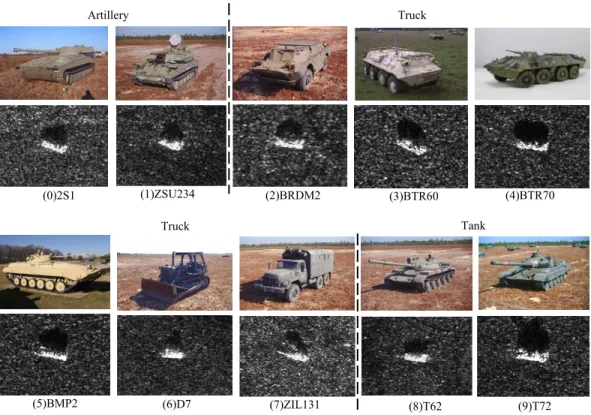
FIGURE 5. Optical images and corresponding SAR images of ten classes of objects in MSTAR dataset.
randomly selected from each sub-dataset to constitute the dataset Dif(i=1,2, . . .n). So in the current iteration, the training set used for training is Df(Df =DL∪D1f∪D2f∪
. . .Dnf). In the training process, the training set is divided into
K batches for training. The current dataset in thej−thbatch is{(x(k),y(k)),k=1,2, . . .m}, wherey(k)represents the real label of the samplex(k). After each batch training, the cross entropy loss is: Lj(j=1,2. . .K)= − 1 m m X k=1 logP(y(k)|x(k);w) (10)
where P(y(k)|x(k);w) represents the recognition probability of the current training sample, mrepresents the number of the samples in the current batch, and w represents all the parameters in the network. We update the network parameters except DSFs byLj. After the completion of multiple batches training, we average the cross entropy loss of all the batches in this iteration: L= 1 K K X j=1 Lj= − 1 K K X j=1 1 m m X k=1 logP(y(k)|x(k);w) (11)
After updating DSFs withL, the network training ends at the current iteration, and the next training iteration starts. The algorithm of DAM is presented in Algorithm 1.
III. EXPERIMENTS AND DISCUSSIONS
In this section, we first describe the dataset used in our experiment and select the baseline model of our method.
After that, the semi-supervised learning experiments are per-formed under unlabeled rate of 20%, 40%, 60%, 80% and 90%. The comparison of the proposed method against several state of the art semi-supervised learning methods is then discussed.
A. DESCRIPTION OF THE DATASET
The MSTAR dataset was collected by the Sandia National Laboratory SAR sensor platform, which was jointly spon-sored by the Defense Advanced Research Projects Agency and the Air Force Research Laboratory [42]. The MSTAR data consists of X-band SAR images with 1-foot by 1-foot resolution. Ten classes of vehicle objects in the MSTAR dataset are chosen in our experiments, which are classified into three categories: artillery, truck, and tank. Artillery classes include 2S1 and ZSU234. Truck classes include BMP2, BRDM2, BTR60, BTR70, D7 and ZIL131. Tank classes include T62 and T72. The SAR and the corresponding optical images of each class are shown in Fig. 5.
For the purpose of testing the generalization ability of our method, the training and testing sets adopt different depression angles. We partition the original training set that contains 2747 SAR target chips in 17◦depression into labeled and unlabeled sample sets under 20%, 40%, 60%, and 80% unlabeled rates. Then, we use the total 2425 SAR target chips in 15◦depression for testing. The data in training and testing sets are with a size of 64∗64 and single channel. Table 1 lists the detailed information of the target chips in this
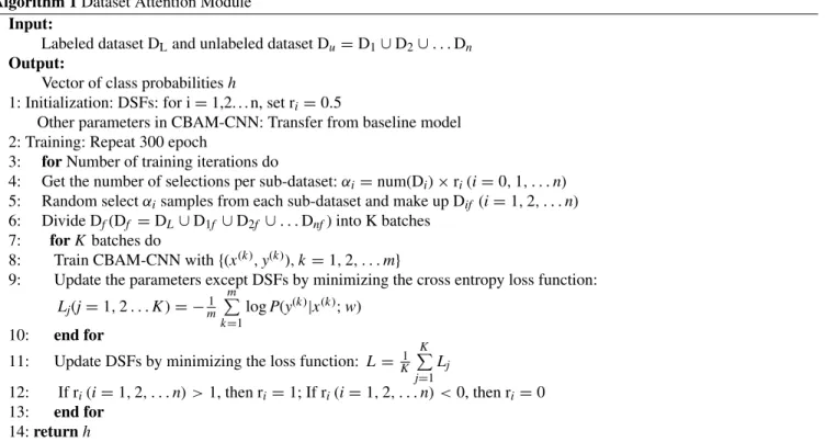
Algorithm 1Dataset Attention Module
Input:
Labeled dataset DLand unlabeled dataset Du=D1∪D2∪. . .Dn
Output:
Vector of class probabilitiesh
1: Initialization: DSFs: for i=1,2. . . n, set ri=0.5
Other parameters in CBAM-CNN: Transfer from baseline model 2: Training: Repeat 300 epoch
3: forNumber of training iterations do
4: Get the number of selections per sub-dataset:αi=num(Di)×ri(i=0,1, . . .n) 5: Random selectαisamples from each sub-dataset and make up Dif (i=1,2, . . .n) 6: Divide Df(Df =DL ∪D1f ∪D2f ∪. . .Dnf) into K batches
7: forK batches do
8: Train CBAM-CNN with{(x(k),y(k)),k=1,2, . . .m}
9: Update the parameters except DSFs by minimizing the cross entropy loss function: Lj(j=1,2. . .K)= −m1 m P k=1 logP(y(k)|x(k);w) 10: end for
11: Update DSFs by minimizing the loss function: L= 1
K K P j=1 Lj 12: If ri(i=1,2, . . .n) >1, then ri=1; If ri(i=1,2, . . .n) <0, then ri=0 13: end for 14:returnh
TABLE 1. Detailed information of the MSTAR dataset used in our experiments.
experiment, and Table 2 lists the specific numbers of labeled and unlabeled samples under different unlabeled rates.
B. SELECTION OF THE BASELINE MODEL
In this section, we will choose the baseline model of our method. CNNs have a rich representation ability, and show remarkable performance in target detection and recogni-tion. For a specific application scenario, designing a new CNN architecture is time-consuming and laborious. There-fore, the baseline model of our method is chosen from the existing model. Here, we compare the performance
of several typical CNN structures, including VGG [15], ResNets [16], [17], DenseNet [18], Inception [19]–[21] and ResNeXt [22]. We use 2747 SAR images at 17◦ degrees to train these models and 2425 SAR images at 15◦ degrees to test. For MSTAR dataset with a small amount of data, there is little difference in training speed between different models. Accuracy is our primary concern. The experimental results are shown in Table 3:
From the experimental results shown in Table 3, we can see that ResNeXt has better accuracy than VGG, ResNets, Inception and DenseNet. ResNeXt exposes a new
dimen-TABLE 2. Specific number of the labeled and unlabeled samples under different unlabeled rates.
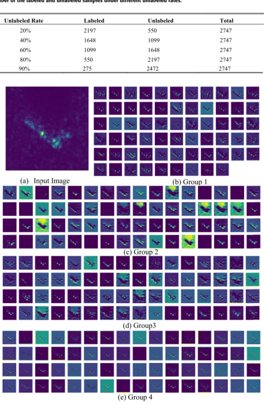
FIGURE 6. (a) is the input image used for testing, and (b, c, d, e) corresponds to the four groups of output feature graphs in the first grouping convolution.
sion, called ‘‘cardinality’’ (the size of the set of transfor-mations). Considering the information in different channels may be localized, cardinality is a way of converting all the channels into grouped convolutions. The group convolu-tion in ResNeXt combines the correlaconvolu-tions between different convolution channels, which is applicable for SAR target
recognition. In the first group convolution layer, there are 512 convolution kernels, which are divided into 8 groups for convolution. Here, we randomly select four groups to demonstrate the process. The results are shown in Fig. 6.
As can be seen from the results shown in Fig. 6, in the same group, the extracted features have much commonness,
TABLE 3. Recognition accuracy comparison between different CNN models.
while the extracted features of different convolution groups are quite different. As shown in Fig. 6(b), in the first group, most of the convolution kernels extract the grayscale features of the input image. The difference between them is that each convolution kernel focuses on different areas and pays dif-ferent attention to the background. The second group shown in Fig. 6(c) extracts the basic contour of the targets: Not only the contour of the SAR ground target, but also the boundary of the shadow. The third group and the fourth group focus on the texture of the input. The texture extracted in the third group is relatively smooth, while the texture extracted from the fourth group is rough. The extracted features by the convolution kernel in different groups are generally different, but there are also some similar features between them. This indicates that there are both connections and difference between SAR image features in different groups. Different features reflect the nature of the targets from different perspectives. The independence effect and joint effect of these features are essential for SAR target recognition.
After the CBAM has been integrated, the information extracted from the ResNeXt is optimized in the convolu-tion module, and the performance of the network is further improved. Therefore, we choose the CBAM-ResNeXt as the baseline model (CBAM-CNN) of our method.
C. EXPERIMENTS UNDER DIFFERENT UNLABELED RATES The experimental part can be shown in two steps. Step 1: training the baseline model and calculating the prediction bias-and-variance of the unlabeled data. Then, the pseudo-label is assigned according to the prediction statistical results. Step 2: DAM is integrated with the baseline model to screen the unlabeled data. On the basis of the baseline model, labeled and unlabeled sets are used to continue the training process. 1) STEP 1: BASELINE MODEL TRAINING AND THE
BIAS-AND-VARIANCE COLLECTING
When training the baseline model on MSTAR dataset, we use the parameters in the baseline model pre-trained on cifar10 optical dataset [43] to initialize the network and fine tune the system on this basis. In the case of a small dataset, fine-tuning can make the network’s recognition accuracy increase rapidly [44]–[46]. When we train the baseline model, only the labeled set is used for training, and all the samples in the testing set are used for testing. We carry out each group of
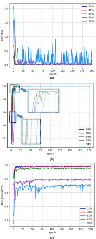
FIGURE 7. Training loss(a), training accuracy(b) and recognition accuracy(c) curves of the baseline model correspond to 20%,40%,60%,80% and 90% unlabeled rate.
experiments with the labeled samples under 20%, 40%, 60%, 80% and 90% unlabeled rates. We record the training loss, the training accuracy and the recognition accuracy of the testing set after each iteration. The experimental results are shown in Fig. 7.
Fig.7 (a) and (b) show that the training loss decreases and the training accuracy increases with the training process. More labeled samples can make the training process converge
FIGURE 8. Bias-and-variance decomposition results under the conditions of 40% ((a), (e)), 60% ((b), (f)), 80% ((c), (g)) and 90% ((d), (h)) unlabeled rates. In the first line ((a), (b), (c), (d)), each point in the graph represents an unlabeled sample. The x and y axes are the bias and variance, and the z axis represents the sum of samples with smaller bias-and-variance; In the below ((e), (f), (g), (h)) is the two-dimensional projection of the left image, with shades representing the number of unlabeled samples.
faster and more smoothly. When the iteration reaches 50, the training accuracy remains 1.0. In order to train adequately and avoid over-fitting, we continue to train for 150 iterations with learning rate decay. In Fig. 7 (c), we can see that the overall accuracy increases as the training iterations increases. With the increase of the unlabeled rates, the amount of the labeled samples in the training set reduces and the infor-mation possessed by these samples correspondingly reduces. As a result, as the unlabeled rates increases, the overall recognition accuracy declines. Especially when the unlabeled rate exceeds 60%, the decrease of accuracy is more sig-nificant, indicating that the feature information possessed by a small amount of the labeled samples is insufficient to represent a part of the target in the testing set. Hence, we need to use unlabeled samples to increase the infor-mation stored on the model, improve the ability of feature extraction and accurately identify more targets in testing set.
As shown in Fig. 7, the recognition accuracy gradually stabilizes during the training process. When the number of the iterations is about 100, the accuracy fluctuation is small. The prediction of the unlabeled data needs to be recorded when the recognition accuracy is stable, so we sustain to train 100 iterations. During these 100 iterations, we input the unlabeled samples into the network for prediction. According to the proposed method, the output of the multiple predictions of the unlabeled data is recorded. After the training of the baseline model, we calculate the bias-and-variance of the unlabeled samples based on the recorded predictions. The bias-and-variance statistical results of the unlabeled data under differ-ent unlabeled rates are shown in Fig. 8.
As shown in Fig. 8, most of the points are near zero bias and variance, which indicates that the network can accurately pre-dict most of the unlabeled samples under 40%, 60%, 80% and 90% unlabeled rate. With the reduction of the labeled data, the range of bias-and-variance fluctuation becomes larger. The bias-and-variance of some unlabeled samples are large, indicating that the predictions of these data are inconsistent in multiple predictions and the target recognition is difficult. Therefore, the unlabeled data should be screened.
After the training of the baseline model, we first assign the pseudo-label to the unlabeled data based on the statistical results of multiple predictions and group the unlabeled data into three sub-datasets. Then these unlabeled sub-datasets and the labeled set are sent into the DA-CBAM and the training is carried out by the baseline model.
2) STEP 2: DA-CBAM TRAINING WITH LABELED AND UNLABELED DATA
It can be seen from the training process of the baseline model shown in Fig. 7 that the best recognition accuracy (99.59%) is basically consistent with supervised learning under 20% unlabeled rate. The reserved labeled samples have mastered enough information, and there is no need to carry out the operation of step 2. We continue to do experiments on 40%, 60%, 80% and 90% unlabeled rates. The training loss and training accuracy are similar to that of step 1 shown in Fig. 7 (a), (b). The recognition accuracy of DA-CBAM during the training process is shown in Fig. 9.
From the final experimental results shown in Fig. 9, we can see that as the number of the training iterations increases, the accuracy of the network recognition is improved. Since
FIGURE 9. Recognition accuracy curves of DA-CBAM correspond to 40%,60%,80% and 90% unlabeled rate.
TABLE 4. Recognition accuracy comparison and recognition accuracy lifting ratio with different unlabeled rates.
our training process continues on the basis of the baseline model, the accuracy increases from the final recognition accuracy of the baseline model. We initialize the DSFs of the three sub-datasets with 0.5, indicating that we initially select 50% of the samples from each sub-dataset to join the training set. We can see that at the beginning of the training, the recognition accuracy fluctuates greatly. With the progress of the training, the composition of the training set is gradually stable, and the accuracy fluctuation is relatively small. The final recognition accuracy of DA-CBAM, and the recognition accuracy increase ratios are shown in Table 4.
From the results, we can see that the DAM has an improve-ment effect on the recognition accuracy. DAM filters out hard-to-learn and redundant samples in the unlabeled set. Compared to the baseline model, DA-CBAM uses the unla-beled samples correctly to enrich the knowledge learned by the network and enables the network to identify more targets in the testing set. With the increase of the unlabeled rates, the features of the unlabeled samples will bring more promo-tional effect to the baseline model trained with limited labeled samples. As a result, the recognition accuracy increases with the increase of the unlabeled rates.
D. COMPARISON EXPERIMENTS WITH OTHER METHODS In this part, we compare the performance of our method with several state of the art semi-supervised learning methods, including Mean-teacher [47], π-model [48], Temporal-ensembling [48] and Ladder-network [49]. In the
mean-teacher, we first apply the moving average of the model parameters into the teacher model, and then gener-ate the proxy label for each unlabeled sample, and finally calculate the overall consistency loss and supervised loss;
π-model learns immutability from the input data by adding two different perturbations and two different regular con-ditions; Temporal-ensembling focuses on the performance of the model in different phases, using different time step integration models. Ladder-network is trained to simultane-ously minimize the sum of the supervised and unsupervised cost functions by backpropagation, avoiding the need for layer-wise pre-training which enables accurate features extraction in a noisy environment.
We carry out experiments under different unlabeled rates. We compare the recognition accuracy of different methods and evaluate it with the receiver operating characteris-tic (ROC) curve [50]. The area under ROC Curve (AUC) values [51] is a comprehensive representative of experimental accuracy and can evaluate the generalization performance of different algorithms. Table 5 shows the recognition accuracy of different methods corresponding to different unlabeled rates. The main configuration of the employed computer are: GPU: GTX 1060; 2.8 GHz; 8GB RAM; operating system: Ubuntu 16.04; running software: Python 3.5. The compu-tational efficiency of the methods is reflected by the aver-age testing time per imaver-age in the last column of Table 5. Fig. 10 shows the ROC curves of different algorithms under different unlabeled rates.
It can be seen from Table 5 that the proposed method has the best recognition accuracy under different unlabeled rates. From the average time per image, we can see that the compu-tational efficiency of these algorithms are of the same order of magnitude. Besides the ladder network, DA-CBAM is faster than the other three algorithms. Further, ResNeXt’s deep and wide network architecture achieves rich feature extraction capability, but at the same time, DA-CBAM offers no par-ticular advantage in computational performance. As shown in Fig. 10, AUC is 1 under the unlabeled rate of 40% and 60%, indicating that almost all the samples in the testing set are accurately identified. DA-CBAM can also maintain high true positive rates and low false positive rates at the unlabeled rates of 80% and 90%. The advantage of DA-CBAM becomes more significant with the increase of the unlabeled rate.
IV. DISCUSSION
The correct usage of the unlabeled data is crucial to semi-supervised learning algorithms. In step 2 of our method, the screened unlabeled set evidently boosts the performance of the network. In this section, we first try to figure out the reasons for the improvement of the network performance. After that, we verify the validity and robustness of DAM through the comparison experiments.
A. NETWORK VISUALIZATION ANALYSIS WITH GRAD-CAM In this section, we make qualitative analysis on DA-CBAM by Grad-CAM (gradient-weighted Class Activation
TABLE 5. Performance comparison of Ladder network, mean-teacher,π-model, temporal-ensembling and our method.
FIGURE 10. ROC curves of recognition accuracy:(a-d) correspond to 40%, 60%, 80% and 90% unlabeled rate, respectively.
Mapping) [52]. Grad-CAM is a visualization method that uses gradients to calculate the importance of spatial positions in a convolution layer. The gradient here is calculated relative to a unique class, and the results of Grad-CAM clearly show the regions involved in the recognition of the target. By comparing the Grad-CAM results of the baseline model and DA-CBAM, we explain how DA-CBAM uses features and improves the accuracy of target recognition. Here, we take the experiment under the 90% unlabeled rate as an example and select two SAR images from the testing set to visualize the results. The two targets correspond to 2S1 and BMP2, respectively. The results are shown in Fig. 11.
In Fig. 11, we use pseudo-colorization for visual analysis. We can see that for the correct recognition labeling, Grad-CAM masks are located at the center of the input image and basically cover the target area. For other non-target
classifications, their recognition areas are disorderly and irregular, and basically do not contain the target areas. The experimental results show that when we use DAM to screen unlabeled data and further train, the recognition accuracy is improved. At the same time, we can see that the network pays more attention to the target area and the area of interest is also increased. DA-CBAM can extract more information from the target area and acquire more features. This indicates that the information in the unlabeled data is used correctly, which can explain why the accuracy of DA-CBAM greatly improves compared with that of the baseline model.
B. VALIDITY AND ROBUSTNESS ANALYSIS OF THE DAM In order to prove the effectiveness of DAM in screening unlabeled data, we conduct the following comparative experi-ment: model-I: DA-CBAM, model-II: training continually on
FIGURE 11. (a), (c) correspond to 2S1 and BMP2 input images, respectively. (b), (d) are the Grad-CAM visualization results of 2S1 and BMP2, and the ten small images upper correspond to the baseline model and the ten small images below correspond to DA-CBAM. The Grad-CAM visualization is calculated for the last convolution outputs. The recognition result is shown on the top of each Grad-CAM mask and the number below them denotes the softmax score of each class.
CBAM only with representative unlabeled data, model-III: training continually on CBAM with all unlabeled data. The specific experiment settings are as shown below.
Here we still take the experiment under 90% unlabeled ratio as an example. First, we use the labeled set to train the baseline model. The first set of the experiments: we integrate DAM with the baseline model and screen the unlabeled set through DAM. The final model DA-CBAM filters out in total 1138 unlabeled samples from the unlabeled set. In the second set of the experiments, we select 1138 unlabeled samples with low prediction bias-and-variance from the unlabeled set and continue to train the same number of iterations directly on the basis of the baseline model. In the third experiment, we employ all the unlabeled data to train the baseline model continuously with the same amount of iterations as the pre-vious two set experiments. We use all the data in the testing set to test, and the recognition accuracy of model-I, model-II and model-III are 93.20%, 92.25%, and 88.52%, respectively. We visually analyze the distribution of unlabeled samples’ predictions through t-SNE (t-Distributed Stochastic Neighbor Embedding) [53]. t-SNE is a nonlinear dimension-reduction algorithm for visualizing high-dimensional data information, which can keep the neighborhood distribution characteris-tics of the high-dimensional data consistent with those of the low-dimensional data. We extract the feature vectors of the testing samples outputted from model-I, model-II and model-III, and then we transform the feature vectors to two-dimensional ones using t-SNE. The result is shown in Fig. 12.
From Fig. 12 we can see that model-I and model-II recognize ten categories of the targets in the testing set. Different categories of samples are mostly divided into dif-ferent regions, while model-III has a fuzzy division. Model-I, which uses DAM for unlabeled data screening, can better predict the samples of the testing set. Samples of different
FIGURE 12. The distribution of the feature vectors output by model-I, model-II and model-III, from left to right (The numbers 0-9 in the figure represent the ten categories of targets in the test set.).
categories are divided into different regions with less over-laps. Model-II retains a large number of representative data, but does not obtain sufficient information from the unlabeled samples. Therefore, it is difficult to identify the data with large difference from the training set. Model-III adds all the unlabeled data into the network for training. In this case, the pseudo-label of some unlabeled data with large bias-and-variance has a high error probability, so using these data directly will have a negative impact on the performance of the network. The third sub-figure in Fig.12 shows that the boundary division between different categories is fuzzy, and the clustering center of each category is not clear, reflecting the low recognition accuracy of the testing set.
In order to fully verify that the DA-CBAM can obtain sufficient information and the network has higher robustness and generalization ability, we add speckle noise [54]–[56] to the testing samples under different variances and test model-I and model-II. Speckle noise is a grainy, black-and-white tex-ture in SAR images [57]–[60]. Testing images with different variance of noise are shown in Fig. 13 and the recognition accuracy of the two models with different noise intensity is shown in Fig. 14.
As can be seen from the experimental results shown in Fig. 13, some detailed information of the SAR target is
FIGURE 13. Original image and images under different Intensity of speckle noise.
FIGURE 14. Recognition accuracy of model-I and model-II under different speckle noise.
submerged by the noise with the increase of noise intensity and the accuracy of the two models declines. Model-I with DAM is more robust to noise and more insensitive to param-eter disturbance. In the second set experiment, unlabeled data with small bias-and-variance are directly adopted. Model-II is more representative, but it can’t fully grasp the information of all unlabeled data. As a result, it is difficult to identify some new data or low-quality targets.
When the DAM is adopted, the screening of the dataset is completed through network learning. In this way, the forma-tion of the training set is more appropriate and the overall generalization ability of the network greatly improves. The DAM is similar to active learning in the extraction of useful samples. The difference is that the samples are assessed by the network itself instead of the expert system, thus avoiding the human participation. And unlike active learning, which uses fixed indicators to select samples, our data screening is accomplished through the network training.
V. CONCLUSION
In order to improve the security of the pseudo-labels assignment and screen the unlabeled data, we propose a semi-supervised learning method based on attention mech-anism and bias-variance decomposition. In view of the characteristics of semi-supervised learning, we propose a novel attention mechanism focusing the data screening, namely DAM. Through the continuous training of the DAM, the model focuses its attention on the useful data, ignores the harmful and useless data. By this way, we select out the data that has a positive effect on network generalization perfor-mance. We use multiple prediction to reduce the uncertainty of single prediction. The pseudo-label of each unlabeled sam-ple is considered to be the classification with the maximum
probability of multiple predictions. The method proposed in this paper is an end-to-end process. At the beginning of the experiment, as long as all the experimental parameters are set, the network can automatically complete the training process, the assignment of pseudo-labels and the unlabeled data screening.
The experiment in this paper is carried out under various unlabeled rates. Compared with the baseline model which only uses labeled samples, the accuracy of the experiment is greatly improved. We have also compared our method with several latest semi-supervised learning algorithms, which shows our method has higher recognition accuracy. After that, we analyze the reason why the accuracy of the final model greatly improves compared with the baseline model through Grad-CAM. The use of unlabeled data enables the network to pay more attention to the target region and enlarge the concerned area. Finally, based on the baseline model, three sets of comparative experiments are carried out to verify the validity and robustness of DAM. The proposed method is a simple yet effective way to select unlabeled samples, which can be widely used to boost the performance of other semi-supervised learning algorithm. The deep and wide network architecture of ResNeXt achieves rich feature extraction capability, at the expense of limited computational efficiency. Use of lightweight networks like MobileNet and ShuffleNet is a promising future research direction. Further, for different tasks, there are hyper-parameters of DAM that need to be preset. More effective and optimised selection of hyper-parameters is another future research challenge, that is of interest.
REFERENCES
[1] G. J. Owirka, S. M. Verbout, and L. M. Novak, ‘‘Template-based SAR ATR performance using different image enhancement techniques,’’Proc. SPIE, Int. Soc. Opt. Eng., vol. 3721, pp. 302–319, 1999.
[2] A. Chatziantoniou, E. Psomiadis, and G. Petropoulos, ‘‘Co-orbital sentinel 1 and 2 for LULC mapping with emphasis on wetlands in a mediterranean setting based on machine learning,’’Remote Sens., vol. 9, no. 12, p. 1259, Dec. 2017.
[3] Q. Zhu, Y. Zhong, S. Wu, L. Zhang, and D. Li, ‘‘Scene classification based on the sparse homogeneous–heterogeneous topic feature model,’’IEEE Trans. Geosci. Remote Sens., vol. 56, no. 5, pp. 2689–2703, May 2018. [4] J. Yang and Z. Peng, ‘‘SAR target recognition based on spectrum feature
of optimal Gabor transform,’’ inProc. Int. Conf. Commun., Circuits Syst. (ICCCAS)., Nov. 2013, vol. 2, pp. 230–234.
[5] F. Gao, F. Ma, Y. Zhang, J. Wang, J. Sun, E. Yang, and A. Hus-sain, ‘‘Biologically inspired progressive enhancement target detection from heavy cluttered SAR images,’’ Cognit. Comput., vol. 8, no. 5, pp. 955–966, Oct. 2016.
[6] S. Chen, H. Wang, F. Xu, and Y.-Q. Jin, ‘‘Target classification using the deep convolutional networks for SAR images,’’IEEE Trans. Geosci. Remote Sens., vol. 54, no. 8, pp. 4806–4817, Aug. 2016.
[7] T. Zhuangzhuang, Z. Ronghui, H. Jiemin, and Z. Jun, ‘‘SAR ATR based on convolutional neural network,’’J. Radars, vol. 5, no. 3, pp. 320–325, Mar. 2016.
[8] F. Gaoet al., ‘‘A new algorithm for sar image target recognition based on an improved deep convolutional neural network,’’Cogn. Comput., vol. 5, pp. 1–16, 2018.
[9] Z. Yueet al., ‘‘A novel semi-supervised convolutional neural network method for synthetic aperture radar image recognition,’’Cogn. Comput., pp. 1–12, 2019.
[10] H.-J. Qi, Y.-G. Wang, J. Ding, and H.-W. Liu, ‘‘SAR target recognition based on multi—Information dictionary learning and sparse representa-tion,’’Syst. Eng. Electron., vol. 37, no. 6, pp. 1280–1287, 2015. [11] W. Lu, Z. Fan, L. Wei, X. Xiao-Ming, and H. Wei, ‘‘A method of SAR target
recognition based on Gabor filter and local texture feature extraction,’’ J. Radars, vol. 4, no. 6, pp. 658–665, 2015.
[12] F. Gao, T. Huang, J. Wang, J. Sun, A. Hussain, E. Yang, ‘‘Dual-branch deep convolution neural network for polarimetric SAR image classification,’’ Appl. Sci., vol. 7, no. 5, p. 447, Apr. 2017.
[13] F. Gao, Y. Zhang, J. Wang, J. Sun, E. Yang, and A. Hussain, ‘‘Visual attention model based vehicle target detection in synthetic aperture radar images: A novel approach,’’Cognit. Comput., vol. 7, no. 4, pp. 434–444, Aug. 2015.
[14] A. Krizhevsky, I. Sutskever, and G. E. Hinton, ‘‘Imagenet classification with deep convolutional neural networks,’’ inProc. Adv. Neural Inf. Pro-cess. Syst., 2012, pp. 1097–1105.
[15] K. Simonyan and A. Zisserman, ‘‘Very deep convolutional networks for large-scale image recognition,’’ Sep. 2014,arXiv:1409.1556. [Online]. Available: https://arxiv.org/abs/1409.1556
[16] K. He, X. Zhang, S. Ren, and J. Sun, ‘‘Deep residual learning for image recognition,’’ inProc. IEEE Conf. Comput. Vis. Pattern Recognit., Jun. 2016, pp. 770–778.
[17] K. He, X. Zhang, S. Ren, and J. Sun, ‘‘Identity mappings in deep residual networks,’’ inProc. Eur. Conf. Comput. Vis., Sep. 2016, pp. 630–645. [18] G. Huang, Z. Liu, L. van der Maaten, and K. Q. Weinberger, ‘‘Densely
connected convolutional networks,’’ inProc. CVPR, Jul. 2017, vol. 1, no. 2, pp. 4700–4708.
[19] C. Szegedy, W. Liu, Y. Jia, P. Sermanet, S. Reed, D. Anguelov, D. Erhan, V. Vanhoucke, and A. Rabinovich, ‘‘Going deeper with convolutions,’’ in Proc. IEEE Conf. Comput. Vis. Pattern Recognit., Jun. 2015, pp. 1–9. [20] C. Szegedy, V. Vanhoucke, S. Ioffe, J. Shlens, and Z. Wojna, ‘‘Rethinking
the inception architecture for computer vision,’’ inProc. IEEE Conf. Comput. Vis. Pattern Recognit. (CVPR), Jun. 2016, pp. 2818–2826. [21] C. Szegedy, S. Ioffe, V. Vanhoucke, and A. A Alemi, ‘‘Inception-v4,
inception-resnet and the impact of residual connections on learning,’’ in Proc. AAAI, Feb. 2017, pp. 4278–4284.
[22] S. Xie, R. Girshick, P. Dollar, Z. Tu, and K. He, ‘‘Aggregated residual transformations for deep neural networks,’’ inProc. Comput. Vis. Pattern Recognit. (CVPR), Jul. 2017, pp. 5987–5995.
[23] X. Zhang, L. Yao, X. Wang, J. Monaghan, D. Mcalpine, and Y. Zhang, ‘‘A survey on deep learning based brain computer interface: Recent advances and new frontiers,’’ May 2019,arXiv:1905.04149. [Online]. Available: https://arxiv.org/abs/1905.04149
[24] Y. Jiao, Y. Zhang, Y. Wang, B. Wang, J. Jin, and X. Wang, ‘‘A novel multilayer correlation maximization model for improving CCA-based fre-quency recognition in SSVEP brain–computer interface,’’Int. J. Neural Syst., vol. 27, no. 8, May 2018, Art. no. 1750039.
[25] N. Liu, L. Wan, Y. Zhang, T. Zhou, H. Huo, and T. Fang, ‘‘Exploiting convolutional neural networks with deeply local description for remote sensing image classification,’’IEEE Access, vol. 6, pp. 11215–11228, 2018.
[26] F. Wang, M. Jiang, C. Qian, S. Yang, C. Li, H. Zhang, X. Wang, and X. Tang, ‘‘Residual attention network for image classification,’’ in Proc. IEEE Conf. Comput. Vis. Pattern Recognit. (CVPR), Jul. 2017, pp. 3156–3164.
[27] J. Hu, L. Shen, S. Albanie, G. Sun, and E. Wu, ‘‘Squeeze-and-excitation networks,’’ Sep. 2017,arXiv:1709.01507. [Online]. Available: https://arxiv.org/abs/1709.01507
[28] S. Woo, J. Park, J.-Y. Lee, and I. S. Kweon, ‘‘Cbam: Convolutional block attention module,’’ inProc. Eur. Conf. Comput. Vision (ECCV), Sep. 2018, pp. 3–19.
[29] B. M. Shahshahani and D. A. Landgrebe, ‘‘The effect of unlabeled samples in reducing the small sample size problem and mitigating the Hughes phenomenon,’’IEEE Trans. Geosci. Remote Sens., vol. 32, no. 5, pp. 1087–1095, Sep. 1994.
[30] Z. Pan, X. Qiu, Z. Huang, and B. Lei, ‘‘Airplane recognition in TerraSAR-X images via scatter cluster extraction and reweighted sparse represen-tation,’’IEEE Geosci. Remote Sens. Lett., vol. 14, no. 1, pp. 112–116, Jan. 2017.
[31] S. Ding, X. Xi, Z. Liu, H. Qiao, and B. Zhang, ‘‘A novel manifold regu-larized online semi-supervised learning model,’’Cognit. Comput., vol. 10, no. 1, pp. 49–61, Feb. 2018.
[32] S. Scardapane and A. Uncini, ‘‘Semi-supervised echo state networks for audio classification,’’Cognit. Comput., vol. 9, no. 1, pp. 125–135, Feb. 2017.
[33] T. Jebara, J. Wang, and S. F. Chang, ‘‘Graph construction and b-matching for semi-supervised learning,’’ inProc. 26th Annu. Int. Conf. Mach. Learn., Jun. 2009, pp. 441–448.
[34] A. Blum and S. Chawla, ‘‘Learning from labeled and unlabeled data using graph mincuts,’’ inProc. Int. Conf. Mach. Learn. (ICML), 2001. [35] A. Blum and T. Mitchell, ‘‘Combining labeled and unlabeled data with
co-training,’’ inProc. 11th Annu. Conf. Comput. Learn. Theory, Jul. 1998, pp. 92–100.
[36] W. Tang, H. Xiong, S. Zhong, and J. Wu, ‘‘Enhancing semi-supervised clustering: A feature projection perspective,’’ inProc. ACM SIGKDD Int. Conf. Knowl. Discovery Data Mining, Aug. 2007, pp. 707–716. [37] M. Bilenko, S. Basu, and R. J. Mooney, ‘‘Integrating constraints and metric
learning in semi-supervised clustering,’’ inProc. 21st Int. Conf. Mach. Learn., Jul. 2004, p. 11.
[38] S. Geman, E. Bienenstock, and R. Doursat, ‘‘Neural networks and the bias/variance dilemma,’’Neural Comput., vol. 4, no. 1, pp. 1–58, Jan. 1992.
[39] R. Kohavi and D. H. Wolpert, ‘‘Bias plus variance decomposition for zero-one loss functions,’’ inProc. ICML, Jul. 1996, vol. 96, pp. 275–283. [40] E. B. Kong and T. G. Dietterich, ‘‘Error-correcting output coding
cor-rects bias and variance,’’ inProc. 12th Int. Conf. Mach. Learn., 1995, pp. 313–321.
[41] G. Valentini, ‘‘An experimental bias-variance analysis of SVM ensem-bles based on resampling techniques,’’IEEE Trans. Syst., Man, Cybern. B. Cybern., vol. 35, no. 6, pp. 1252–1271, Dec. 2005.
[42] The Air Force Moving and Stationary Target Recognition Database. Available. Accessed: Feb. 3, 2016. [Online]. Available: https://www.sdms.afrl.af.mil/datasets/mstar/
[43] A. Krizhevsky and G. Hinton, ‘‘Learning multiple layers of features from tiny images,’’ Tech. Rep., 2009, vol. 1, no. 4, p. 7.
[44] D. Mishkin and J. Matas, ‘‘All you need is a good init,’’ Nov. 2015, arXiv:1511.06422. [Online]. Available: https://arxiv.org/abs/1511.06422 [45] J. Yosinski, J. Clune, Y. Bengio, and H. Lipson, ‘‘How transferable are
features in deep neural networks?’’ inProc. Adv. Neural Inf. Process. Syst., 2014, pp. 3320–3328.
[46] S. J. Pan and Q. Yang, ‘‘A survey on transfer learning,’’IEEE Trans. Knowl. Data Eng., vol. 22, no. 10, pp. 1345–1359, Oct. 2010.
[47] A. Tarvainen and H. Valpola, ‘‘Mean teachers are better role models: Weight-averaged consistency targets improve semi-supervised deep learn-ing results,’’ inProc. Adv. Neural Inf. Process. Syst., 2017, pp. 1195–1204. [48] S. Laine and T. Aila, ‘‘Temporal ensembling for semi-supervised learning,’’ Oct. 2016, arXiv:1610.02242. [Online]. Available: https://arxiv.org/abs/1610.02242
[49] A. Rasmus, M. Berglund, M. Honkala, H. Valpola, and T. Raiko, ‘‘Semi-supervised learning with ladder networks,’’ inProc. Adv. Neural Inf. Pro-cess. Syst., 2015, pp. 3546–3554.
[50] T. Fawcett, ‘‘ROC graphs: Notes and practical considerations for researchers,’’Mach. Learn., vol. 31, no. 1, pp. 1–38, Mar. 2004. [51] A. P. Bradley, ‘‘The use of the area under the ROC curve in the
evalu-ation of machine learning algorithms,’’Pattern Recognit., vol. 30, no. 7, pp. 1145–1159, Jul. 1997.
[52] R. R. Selvaraju, M. Cogswell, A. Das, R. Vedantam, D. Parikh, and D. Batra, ‘‘Grad-CAM: Visual explanations from deep networks via gradient-based localization,’’ CoRR, vol. abs/1610.02391, Oct. 2016, pp. 1–24.
[53] L. J. P. van der Maaten and G. E. Hinton, ‘‘Visualizing data using T-SNE,’’ J. Mach. Learn. Res., vol. 9, pp. 2579–2605, Nov. 2008.
[54] J. W. Goodman, ‘‘Some fundamental properties of speckle,’’J. Opt. Soc. Amer., vol. 66, no. 66, pp. 1145–1150, 1976.
[55] F. Gao, Y. Zhang, J. Wang, and J. Sun, ‘‘Fast algorithm for inverse two-dimensional s transform and its application in time-frequency filtering for SAR image despeckling,’’Chin. J. Electron., vol. 25, no. 1, pp. 100–105, Jan. 2016.
[56] F. Gao, X. Xue, J. Sun, J. Wang, and Y. Zhang, ‘‘A SAR image despeckling method based on two-dimensional S transform shrinkage,’’IEEE Trans. Geosci. Remote Sens., vol. 54, no. 5, pp. 3025–3034, May 2016. [57] F. T. Ulaby, R. K. Moore, and A. K. Fung, ‘‘Microwave remote sensing:
[58] F. T. Ulaby, T. F. Haddock, and R. T. Austin, ‘‘Fluctuation statistics of millimeter-wave scattering from distributed targets,’’IEEE Trans. Geosci. Remote Sens., vol. 26, no. 3, pp. 268–281, May 1988.
[59] J. Zhang and N. Tansu, ‘‘Optical gain and laser characteristics of InGaN quantum wells on ternary InGaN substrates,’’IEEE Photon. J., vol. 5, no. 2, Apr. 2013, Art. no. 2600111.
[60] F. Gao, F. Ma, J. Wang, J. Sun, E. Yang, and H. Zhou, ‘‘Visual saliency modeling for river detection in high-resolution SAR imagery,’’IEEE Access, vol. 6, pp. 1000–1014, 2018.
FEI GAO received the B.S. and M.S. degrees from the Xi’an Petroleum Institute, Xi’an, China, in 1996 and 1999, respectively, and the Ph.D. degree from the Beijing University of Aeronau-tics and AstronauAeronau-tics (BUAA), Beijing, China, in 2005.
He is currently an Associate Professor with the School of Electronic and Information Engineering, BUAA. He is interested in radar signal processing, moving target detection, and image processing.
WEI SHIreceived the B.S. degree in electronic and information engineering from the Beijing Uni-versity of Aeronautics and Astronautics, Beijing, China, in 2018, where he is currently pursuing the M.S. degree.
His research interests include radar signal pro-cessing, image propro-cessing, machine learning, and target detection.
JUN WANGreceived the B.S. degree from North western Polytechnical University, Xi’an, China, in 1995, and the M.S. and Ph.D. degrees from the Beijing University of Aeronautics and Astronau-tics (BUAA), Beijing, China, in 1998 and 2001, respectively.
He is currently a Professor with the School of Electronic and Information Engineering, BUAA. He is interested in signal processing, DSP/FPGA real-time architecture, target recognition and tracking, and so on. His research has resulted in 38 papers in journals, books, and conference proceedings.
AMIR HUSSAINreceived the B.Eng. and Ph.D. degrees in electronic and electrical engineering from the University of Strathclyde, Scotland, U.K., in 1992 and 1997, respectively. He held postdoc-toral and academic positions at the West of Scot-land, from 1996 to 1998, Dundee, from 1998 to 2000, and Stirling Universities, from 2000 to 2018, respectively. He is currently a Professor and the Founding Head of the Cognitive Big Data and Cybersecurity (CogBiD) Research Labora-tory, Edinburgh Napier University, U.K. His research interests include cog-nitive computation, machine learning, and computer vision.
HUIYU ZHOUreceived the B.Eng. degree in radio technology from the Huazhong University of Sci-ence and Technology, Wuhan, China, the M.S. degree in biomedical engineering from the Uni-versity of Dundee, Dundee, U.K., and the Ph.D. degree in computer vision from Heriot-Watt Uni-versity, Edinburgh, U.K.
He is currently a Reader with the Department of Informatics, The University of Leicester, Leices-ter, U.K. He has taken part in the consortiums of a number of research projects in medical image processing, computer vision, intelligent systems, and data mining.