A P P R O X I M AT I O N S C H E M E S F O R M A C H I N E S C H E D U L I N G m a r t e n m a a c k
Dissertation
zur Erlangung des akademischen Grades Doktor der Naturwissenschaften
(Dr. rer. nat.) der Technischen Fakultät
der Christian-Albrechts-Universität zu Kiel eingereicht im Jahr2019
2. g u ta c h t e r Prof. Dr. Friedhelm Meyer auf der Heide 3. g u ta c h t e r Prof. Dr. Asaf Levin
d at u m d e r d i s p u tat i o n 7. Mai2020
Marten Maack:Approximation Schemes for Machine Scheduling,c Novem-ber2019
A B S T R A C T
In the classical problem of makespan minimization on identical par-allel machines, or machine scheduling for short, a set of jobs has to be assigned to a set of machines. The jobs have a processing time and the goal is to minimize the latest finishing time of the jobs. Ma-chine scheduling is well known to be NP-hard and thus there is no polynomial time algorithm for this problem that is guaranteed to find an optimal solution unless P=NP. There is, however, a polynomial time approximation scheme (PTAS) for machine scheduling, that is, a family of(1+ε)-approximations for eachε > 0. Whether a problem admits an approximation scheme or not is a fundamental question in approximation theory. In the present work, we consider this question for several variants of machine scheduling.
For instance, we study the problem where the machines are par-titioned into a constant number of types and the processing time of the jobs is also dependent on the machine type it is assigned to. We present an efficient PTAS (EPTAS)—a PTAS whose running time is
a product of some function in 1/ε and a polynomial in the input
length—for this problem and variants thereof.
In the restricted assignment problem, each job may only be assigned to a given subset of machines. We show that certain cases of restricted assignment do not admit a PTAS unless P=NP, e.g., the case in which the machines are linearly ordered and each job is eligible on a set of consecutive machines. Moreover, we introduce a graph framework based on the restrictions of the jobs and use it in the design of ap-proximation schemes for several variants of restricted assignment generalizing and unifying many of the known PTAS results.
Furthermore, we introduce an enhanced integer programming for-mulation for assignment problems, show that it can be efficiently solved, and use it in the EPTAS design for variants of machine schedul-ing with setup times. For one of the problems, we show that there is also a PTAS in the case with uniform machines, where machines have speeds influencing the processing times of the jobs.
Lastly, we consider cases in which each job requires a certain amount of a shared renewable resource and the processing time is depended on the amount of resource it receives or not. We present asymptotic fully polynomial time approximation schemes (AFPTAS) for the problems: For anyε > 0a schedule is provided whose length lies within a factor of(1+ε)of the optimum value except for an additional additive error depending on the maximal processing time and1/ε.
Z U S A M M E N FA S S U N G
Im klassischen Problem des Machine Scheduling muss eine Menge von Jobs einer Menge von Maschinen zugewiesen werden. Die Jobs haben eine Bearbeitungszeit und das Ziel ist es, den Zeitpunkt zu minimieren an dem der letzte Job vollständig bearbeitet ist. Machine Scheduling ist NP-vollständig und daher gibt es keinen Algorithmus, der in polynomieller Zeit garantiert eine optimale Lösung für das Problem findet, es sei denn P=NP. Es gibt jedoch ein Approximationsschema mit polynomieller Laufzeit (PTAS) für Machine Scheduling, d.h. eine Familie von(1+ε)-Approximationen für jedesε > 0. Ob ein Problem ein Approximationsschema zulässt oder nicht, ist eine grundlegende Frage der Approximationstheorie. In dieser Arbeit betrachten wir diese Frage für mehrere Varianten des Machine Scheduling.
So betrachten wir beispielsweise Varianten, bei denen die Maschi-nen in eine konstante Anzahl von Typen partitioniert sind und die Bearbeitungszeit der Jobs vom Maschinentyp abhängt. Wir präsentie-ren ein effizientes PTAS (EPTAS) für dieses Problem, d.h. ein PTAS dessen Laufzeit durch das Produkt einer Funktion in 1/εund eines Polynoms in der Eingabelänge abgeschätzt werden kann.
Bei dem Restricted Assignment Problem darf jeder Job nur einer gegebenen Teilmenge von Maschinen zugeordnet werden. Wir zeigen, dass bestimmte Spezialfälle von Restricted Assignment kein PTAS zulassen (sofern P6=NP), z.B. der Fall, in dem die Maschinen line-ar geordnet sind und jeder Job auf einer Menge von konsekutiven Maschinen zulässig ist. Weiterhin führen wir ein auf den Zulässig-keiten basierendes Graphen-Framework ein und verwenden es beim PTAS-Design für diverse Varianten des Restricted Assignment.
Darüber hinaus entwickeln wir eine erweiterte ganzzahlige Op-timierungsformulierung für Zuweisungsprobleme, zeigen, dass sie effizient gelöst werden kann, und verwenden sie im EPTAS-Design für Varianten von Machine Scheduling mit Setup Zeiten. Für eine dieser Varianten zeigen wir zusätzlich, dass es auch für den Fall mit uniformen Maschinen ein PTAS gibt. Uniforme Maschinen haben Geschwindigkeiten, die die Bearbeitungszeiten der Jobs beeinflussen.
Schließlich betrachten wir Fälle, in denen jeder Job eine bestimm-te Menge einer gebestimm-teilbestimm-ten erneuerbaren Ressource benötigt und die Bearbeitungszeit von der Menge der erhaltenen Ressource abhängt oder nicht. Wir präsentieren asymptotische, vollständig polynomielle Approximationsschemata (AFPTAS) für die Probleme: Für jedesε > 0
wird ein Schedule gefunden dessen Länge, bis auf einen zusätzlichen additiven Fehler abhängig von der maximalen Ausführungszeit und
1/ε, höchstens um einen Faktor von(1+ε)vom Optimum abweicht.
P U B L I C AT I O N S
The present work is based on the following publications:
[78] Klaus Jansen and Marten Maack. “An EPTAS for Scheduling on Unrelated Machines of Few Different Types.” In:Algorithmica 81.10(2019), pp.4134–4164.doi:
10.1007/s00453-019-00581-w.
[79] Klaus Jansen, Marten Maack, and Alexander Mäcker.
“Schedul-ing on (Un-)Related Machines with Setup Times.” In: 2019
IEEE International Parallel and Distributed Processing Symposium, IPDPS2019, Rio de Janeiro, Brazil, May20-24,2019.2019, pp.145– 154.doi:10.1109/IPDPS.2019.00025.
[81] Klaus Jansen, Marten Maack, and Malin Rau. “Approximation Schemes for Machine Scheduling with Resource (In-)dependent Processing Times.” In:ACM Trans. Algorithms15.3(2019), 31:1– 31:28.doi:10.1145/3302250.
[82] Klaus Jansen, Marten Maack, and Roberto Solis-Oba. “Struc-tural Parameters for Scheduling with Assignment Restrictions.” In: Algorithms and Complexity - 10th International Conference, CIAC2017, Athens, Greece, May24-26, 2017, Proceedings.2017, pp.357–368.doi:10.1007/978-3-319-57586-5\_30.
[86] Klaus Jansen, Kim-Manuel Klein, Marten Maack, and Malin Rau. “Empowering the Configuration-IP - New PTAS Results for Scheduling with Setups Times.” In:10th Innovations in The-oretical Computer Science Conference, ITCS 2019, January10-12, 2019, San Diego, California, USA.2019,44:1–44:19.doi:10.4230/
LIPIcs.ITCS.2019.44.
[111] Marten Maack and Klaus Jansen. “Inapproximability Results for Scheduling with Interval and Resource Restrictions.” In: 37th International Symposium on Theoretical Aspects of Computer Science, STACS 2020, March 10-13, 2020, Montpellier, France. Vol.154.2020,5:1–5:18.doi:10.4230/LIPIcs.STACS.2020.5. All of the above publications have been peer-reviewed. Conference versions of [78] and [81] have previously been published in the pro-ceedings of WADS2017[77] and SODA2016[80], respectively.
A C K N O W L E D G M E N T S
I sincerely thank my advisor Klaus Jansen for supporting this work. Many thanks to my other colleagues in the algorithms and complexity group in Kiel, namely, Sebastian Berndt, Max Deppert, Kilian Grage, Ute Iaquinto, Maren Kaluza, Kim-Manuel Klein, Stefan Kraft, Felix and Kati Land, Alexandra Lassota, Parvaneh Massouleh, Niklas Paulsen, Malin Rau, and Lars Rohwedder. I had a marvelous time collaborating, traveling, debating, and working along side with you day to day.
As part of my studies, I visited the Western University in London, Ontario for six months. I wish to thank Roberto Solis-Oba for super-vising my work during that time and for generally being a great host. Thanks also to Daniel Page with whom I collaborated while visiting and shared an office as well as many exciting conversations.
I would like to thank all my co-authors with whom I have worked on the papers contributing to this work, namely, Klaus Jansen, Kim-Manuel Klein, Alexander Mäcker, Malin Rau, and Roberto Solis-Oba. A special thanks goes to Kim-Manuel Klein, Alexandra Lassota, and Daniel Page for proofreading parts of this work.
Finally, I thank my family and friends, and especially my wife Beate, my mother Gabi, and my father Rainer for their unconditional support and advice, and for generally putting up with me.
C O N T E N T S
1 i n t r o d u c t i o n 1 2 p r e l i m i na r i e s 9
2.1 Basic Concepts and Notation 9
2.2 Example Approximation Scheme 11
3 u n r e l at e d s c h e d u l i n g w i t h f e w t y p e s 15
3.1 Introduction 15
3.2 Basic EPTAS 19
3.3 Better running time 23
3.4 The Santa Claus Problem 30
3.5 Uniform Machine Types 33
3.6 Vector Scheduling 40 3.7 Open Problems 43 4 i n t e r va l a n d r e s o u r c e r e s t r i c t i o n s 45 4.1 Introduction 45 4.2 Interval Restrictions 49 4.3 Resource Restrictions 63 4.4 Open Problems 73 5 s t r u c t u r a l pa r a m e t e r r e s t r i c t i o n s 75 5.1 Introduction 75 5.2 Preliminaries 78 5.3 Treewidth Results 80
5.4 Clique- and Rankwidth Results 88
5.5 Other Objective Functions 97
5.6 Open Problems 99 6 m a c h i n e s c h e d u l i n g w i t h s e t u p t i m e s 101 6.1 Introduction 101 6.2 Preliminaries 105 6.3 Module Configuration IP 107 6.4 EPTAS results 110
6.5 Improvements of the running time 133
6.6 Open Problems 136 7 u n i f o r m s c h e d u l i n g w i t h s e t u p t i m e s 137 7.1 Introduction 137 7.2 PTAS 137 7.3 Open Problems 150 8 m a c h i n e s c h e d u l i n g w i t h a s h a r e d r e s o u r c e 151 8.1 Introduction 151
8.2 Single resource constrained scheduling 155
8.3 Resource Dependent Processing Times 175
8.4 Open Problems 185
b i b l i o g r a p h y 187
1
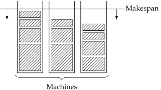
I N T R O D U C T I O NConsider the problem of makespan minimization on identical parallel machines, called machine scheduling for short: Given a set M of m
machines and a set Jofnjobs each with a processing time or sizepj, the goal is to find an assignmentσ:J→Mof the jobs to the machines such that the maximal load any machine receives is minimized (see Figure1.1). The maximal loadCmax(σ) =maxi∈MP
j∈σ−1(i)pj is also
called themakespanandσaschedule. Machine scheduling is a classical combinatorial optimization problem—problems with a discrete and usually finite space of feasible solutions in which the goal is to find an optimal solution with respect to a given objective function. Like for many combinatorial optimization problems, the study of machine scheduling can be motivated from practical applications, e.g., from scheduling in production facilities or the assignment of computational tasks to identical processors. On the other hand, their simple combina-torial structure arguably already motivates their study from a purely theoretical perspective. In this work, we study algorithms for problems closely related to machine scheduling. We focus on the theoretical perspective, but consider many variants that capture additional diffi-culties that typically arise in practice, like, e.g., assignment restrictions, setup times or the influence of additional resources.
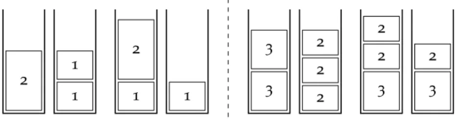
a l g o r i t h m s f o r m a c h i n e s c h e d u l i n g. Finding a sensible assignment for a given machine scheduling instance is not very hard. For example, one could simply consider one job after another and assign it to a machine that so far received minimal load. We call this heuristic algorithmheuin the following. However, the solutions generated by this procedure will usually not be optimal (see Figure 1.2). One could improve the procedure by first sorting the jobs by
Makespan
Machines
Figure1.1: A schedule for a machine scheduling instance with11jobs and3
machines. The jobs are represented by the hatched rectangles.
2 1 1 1 2 1 3 3 2 2 2 3 2 2 3 2
Figure1.2: Two simple examples visualizing that heu and heu∗ are not
guaranteed to find optimal solutions. In the example on the left, an optimal solution is depicted left and the solution produced by
heuwhen the big job is considered last on the right. On the right,
again an optimal solution is depicted left and a solution produced by heu∗on the right. The depicted numbers correspond to the
processing times.
decreasing processing times, but still the generated solutions are not guaranteed to be optimal (see Figure 1.2). We call the improved heuristicheu∗.
On the other hand, it is also not particularly difficult to find an optimal solution—we could try each of the mmachine as the place of assignment for each of the n jobs yielding mn possibilities. We can improve upon this brute force approach, e.g., by using a dynamic program in which the machines are considered one after another and a best partial solution for each subset of jobs is remembered. This approach yields a running time of 2O(n)m (see Section 5.2). While there are more elaborate known approaches to solve this problem, they all share the property that their running time is exponential in the input length. Therefore, they scale very badly: Say we had an algorithm with running time 2nand an instance that is solved by it in
1second. Then adding 10jobs increases the running time to a quarter hour, another10 to a dozen days, another10 to a few decades, and adding60jobs in total would give a running time that is much longer than the estimated age of the earth. The heuristic proceduresheuand heu∗, on the other hand, have a running time that is at most quadratic in the input length, that is, increasing the number of jobs by afactorof
60would give a running time of at most an hour in a corresponding sample calculation.
p v s. n p. Algorithms whose running times are bounded by linear or quadratic functions in the input length are deemed desirable in most contexts. However, considering the asymptotic scaling behaviour, any polynomial is preferable to any exponential function. Indeed, the question of whether a problem admits a polynomial time algorithm is considered fundamental in theoretical computer science. An early discussion of this idea can be found in a work by Edmonds [41] from
1965, who studied a polynomial time algorithm for the maximum
i n t r o d u c t i o n 3
There is an obvious finite algorithm, but that algorithm increases in difficulty exponentially with the size of the graph. It is by no means obvious whetheror notthere exists an algorithm whose difficulty increases only algebraically [i.e., polynomially] with the size of the graph.
The mathematical significance of this paper rests largely on the assumption that the two preceding sentences have mathematical meaning.[...]
For practical purposes the difference between algebraic and exponential order is often more crucial than the differ-ence between finite and non-finite.
In the early 1970s, Cook [33] and Karp [91] introduced the class of NP-complete decision problems1
, which are widely believed not to admit (deterministic) polynomial time algorithms. The class of decision problems that can be solved in polynomial time is denoted as P, while NP denotes the class of decision problems for which, roughly speaking, there exist solutions for positive instances that can beverified in polynomial time. The former class is a subclass of the latter, and P6=NP is a widely accepted and famous conjecture. Resolving it is one of the so called Millennium Prize Problems—a collection of problems in mathematics that are considered to be particularly important and hard. Now, a problem is called NP-complete if it is both in NP and NP-hard. The latter property essentially means that a polynomial time algorithm for any of them would imply such an algorithm for all problems in NP2
. Many fundamental problems are well-known to be NP-complete including the decision versions3
of numerous combinatorial optimization problems (see [51]). This is also the case for machine scheduling. Since solving the optimization version implies solving the decision version of a problem, there is no polynomial time algorithm for machine scheduling that is guaranteed to find an optimal solution unless P=NP. However, there are intriguing approaches to deal with this problem.
a p p r o x i m at i o n a l g o r i t h m s. Consider the heuristic algorithms heu and heu∗. Both algorithms assign each job to a least loaded machine, and therefore no machine may receive more load than the average load and one additional job which may have maximal size. Hence, the load of each machine is upper bounded by maxj∈Jpj+ (Pj∈Jpj)/m. Both maxj∈Jpj and(
P
j∈Jpj)/mare lower bounds for the optimal objective value, and therefore the objective value of a solution produced by the heuristics is at most twice as big as the optimal one.
1 Problems for which a yes-or-no question has to be answered.
2 For proper definitions and background information on complexity theory, we refer to the textbook by Arora and Barak [8].
3 For optimization problems, one can state the question of whether a solution with at most/at least a certain objective value exists.
Letalg(I)denote the objective value an algorithmalg computes for an input instanceIandopt(I)be the corresponding optimal value. An algorithmalg is calledapproximation algorithmwithratioαorα -approximation ifalg(I)6αopt(I)in case of a minimization problem orαalg(I)>opt(I)in case of a maximization problem. The ratio α is also called theapproximation guaranteeorrateof the algorithm. Fur-thermore, if not stated otherwise, we use the term approximation algorithm as a short hand for polynomial time approximation algo-rithm. Using the above notation, the heuristics heu and heu∗ are
2-approximations.
The concept of approximation algorithms was formally introduced by Johnson [87] in1974, however, there were earlier results proving approximation guarantees of algorithms. For instance, in1966and1969 Graham [57,58] considered the heuristicsheuandheu∗and proved them to be2- and4/3-approximations, respectively. The algorithmheu is usually calledlist schedulingand the prioritization of large jobs used inheu∗is known as theLPT(largest processing time first) rule . These are considered among the first results in the field of approximation algorithms.
When studying approximation algorithms, it is rather natural to ask which is the best possible approximation ratio one could obtain for a given problem or even whether there exists a best ratio. For machine scheduling, the answer to the latter question turns out to be negative. a p p r o x i m at i o n s c h e m e s. For a given problem, apolynomial time approximation scheme (PTAS)is a family of algorithms that includes a (1+ε)-approximation for each ε > 0. We also study approximation schemes with higher requirements on the running time. In particular, a PTAS is calledefficient(EPTAS) if it has a running time of the form
f(1/ε)|I|O(1), wherefis some computable function and|I| the input length. Furthermore, an EPTAS is calledfully polynomial(FPTAS) if the functionfis a polynomial.
Whether a problem admits a PTAS or not is a fundamental question in approximation. In 1987, Hochbaum and Shmoys [65] designed a PTAS for machine scheduling and hence showed that any approxima-tion guarantee strictly above1can be achieved for this problem4
. Since then, there have been many more results concerning approximation schemes for machine scheduling and variants thereof (like, e.g., [5,46, 47,66,72,73,119,122,133]).
The present work aims at deepening the understanding in this line of research. To this end, we design approximation schemes for many important variants of machine scheduling. We introduce new techniques in this context and show that our results work for a wide variety of problems. Furthermore, we present inapproximability
re-4 We present an example PTAS for machine scheduling in Section2.2which is closely related to this result.
i n t r o d u c t i o n 5
sults that rule out the existence of approximation schemes for certain cases under the assumption that P6=NP.
c l a s s i c a l s c h e d u l i n g p r o b l e m s. In order to discuss the re-sults of this work in more detail, we first have to introduce some classical variants of machine scheduling studied in the literature. The
most common two are called makespan minimization on uniformly
relatedandunrelatedparallel machines, and are abbreviated asuniform andunrelated schedulingin the following. In the problem of unrelated scheduling, the processing time of a job depends on the machine it is processed on, that is, the input includes a processing timepijfor each machineiand jobj. Uniform scheduling can be seen as a special case of unrelated scheduling where each jobjhas a sizepj, each machinei
a speedsi, and the processing time of jobjon machineiis given by
pij=pj/si.
For uniform scheduling, there is a PTAS due to Hochbaum and Shmoys [66], and both machine [5] and uniform scheduling [72] are known to admit an EPTAS. On the other hand, the problems are well known to be strongly NP-hard5
, which implies that there is no FPTAS for them unless P=NP. If the number of machines is considered con-stant, already unrelated scheduling admits an FPTAS [67]. However, there is no approximation algorithm with a ratio smaller than 1.5
for unrelated scheduling unless P=NP. This was shown by Lenstra, Shmoys and Tardos [108] and already holds for the so calledrestricted assignmentproblem, where each job has a sizepjandpij∈{pj,∞}. For each jobj, the machinesiwithpij=pjare called eligible and we say that the assignment ofjto other machines is restricted. Lestra et al. also provided a2-approximation for unrelated scheduling. Closing (or nar-rowing) the gap between1.5-inapproximability and2-approximation for either unrelated scheduling or restricted assignment is considered one of the most important open problems in approximation [145] and scheduling theory [132]. This also motivates the study of special cases, and whether these cases admit approximation schemes in particular, in order to better understand the approximability of these problems.
For a broader overview of scheduling theory, we refer to the follow-ing textbook [127] and survey [28].
c o n t r i b u t i o n s a n d o r g a n i z at i o n
In Chapter 2, we discuss further basic concepts and notation and present an example PTAS for machine scheduling. Each of the remain-ing chapters is based on a prior publication and can, for the most part, be read independently. Exceptions to this rule are Chapter 5 and 7 which are closely related to the respective direct predecessor chap-ters and therefore cover the related literature and motivation of the
work only to a limited extent. In the following, we briefly discuss the problems considered in each chapter as well as the obtained results. c h a p t e r 3. In this chapter, we consider the variant of unrelated scheduling with a constant numberKof machine types. Two machines have the same type if all jobs have the same processing time for them. Note that forK=1, we have the problem of machine scheduling. We present an EPTAS for the problem with a running time of
2O(Klog(K)1/εlog4 1/ε)+
poly(|I|),
where|I|denotes the input length. Furthermore, we study three other problem variants and present an EPTAS for each of them: The Santa Claus problem, where the minimum machine load has to be maxi-mized; the case of unrelated scheduling with a constant number of uniformtypes, where machines of the same type behave like uniform machines; and the multidimensional vector scheduling variant of the problem, where both the dimension and the number of machine types are constant. For the Santa Claus problem we achieve the same asymp-totic running time. The results are obtained, using mixed integer linear programming and rounding techniques. This chapter is based on [77]. c h a p t e r 4. We consider two variants of the restricted assignment problem. In the case of interval restrictions the machines can be totally ordered such that jobs are eligible on consecutive machines. We show that there is no PTAS unless P=NP for this variant. The question of whether a PTAS for this problem exists was stated as an open problem before, and PTAS results for special cases of this variant are known. Interestingly, there is a paper claiming to have found a PTAS for this problem but it is flawed.
Furthermore, we consider a variant with resource restrictions where the sets of eligible machines are of the following form: There is a fixed number of (renewable) resources, each machine has a capacity, and each job a demand for each resource. A job is eligible on a machine if its demand is at most as big as the capacity of the machine for each resource. For one resource, this problem has been intensively studied under several different names and is known to admit a PTAS, and for two resources the variant with interval restrictions is contained as a special case. Moreover, the version with multiple resources is closely related to unrelated scheduling with a low rank processing time matrix. We show that there is no polynomial time approximation algorithm with a rate smaller than48/47≈1.02or1.5for scheduling with resource restrictions with2 or4 resources, respectively, unless P=NP. All our results can be extended to the Santa Claus variants of the problems where the goal is to maximize the minimal processing time any machine receives. This chapter is based on [111].
i n t r o d u c t i o n 7
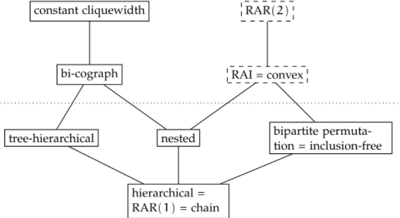
c h a p t e r 5. Similar to the previous chapter, we consider special types of assignment restrictions. We introduce a graph framework based on the restrictions:
In the primal graph, the jobs are the nodes and are adjacent if they share an eligible machine. In the dual graph, on the other hand, the machines are the nodes and two machines are adjacent if there is a job that is eligible on both of them. Lastly, the incidence graph is a bipartite graph that includes both jobs and machines as nodes, and a job node is adjacent to a machine node if the job is eligible on the machine. We study cases in which these graphs have certain structural properties.
We show that the variant of restricted assignment where the inci-dence graph has a constant rank- or cliquewidth admits a PTAS. This generalizes and unifies several known PTAS results.
Furthermore, we consider the treewidth for each of the three graphs. We show that a constant treewidth for the dual or incidence graph implies the existence of an FPTAS. Furthermore, we design so called fixed parameter tractable (FPT) algorithms, that is, exact algorithms with a running time of the formf(c)poly(|I|)wherecis a parameter of the instanceI,fsome computable function, and|I| the input length. We present FPT results for each of the three graph. For instance, we show that restricted assignment is FPT with respect to the treewidth of the primal graph. All results concerning the treewidth also work for the more general case of unrelated scheduling with restrictions. This chapter is based on [82].
c h a p t e r 6. Integer linear programs of configurations, or configura-tion IPs, are a classical tool in the design of algorithms for scheduling and packing problems where a set of items has to be placed in mul-tiple target locations. Herein, a configuration describes a possible placement on one of the target locations, and the IP is used to choose suitable configurations covering the items. We present an augmented IP formulation, which we call the module configuration IP. It can be described within the framework of n-fold integer programming and, therefore, be solved efficiently. As an application, we consider variants of machine scheduling with setup times. For instance, we investigate the case that jobs can be split and scheduled on multiple machines. However, before a part of a job can be processed, an uninterrupted setup depending on the job has to be paid. For both of the variants that jobs can be executed in parallel or not, we obtain an efficient polynomial time approximation scheme (EPTAS) of running time
f(1/ε)poly(|I|)with a single exponential term inffor the first and a double exponential one for the second case. Previously, only constant factor approximations of 5/3and 4/3+ε, respectively, were known. Furthermore, we present an EPTAS for a problem where classes of (non-splittable) jobs are given, and a setup has to be paid for each
class of jobs being executed on one machine. This chapter is based on [86].
c h a p t e r 7. In this chapter, we consider the variant of uniform scheduling in which the jobs are partitioned into classes and class depended setup has to be paid for each class present on a machine. This is the uniform version of the non-splittable problem considered in the last chapter. We design a PTAS for this problem. This chapter is based on parts of [79].
c h a p t e r 8. We consider two related variants of machine schedul-ing: single resource constrained scheduling on identical parallel ma-chines and a generalization with resource dependent processing times. In both problems, jobs require a certain amount of an additional resource and have to be scheduled on machines minimizing the makespan, while at every point in time a given resource capacity is not exceeded. In the first variant of the problem, the processing times and resource amounts are fixed, while, in the second, the former depends on the latter.
Both problems contain the problem of bin packing with cardinality constraints as a special case, and, therefore, these problems are strongly NP-complete even for a constant number of machines larger than three, which can be proven by a reduction from3-Partition. Furthermore, if the number of machines is part of the input, we cannot hope for an approximation algorithm with absolute ratio smaller than3/2.
We present asymptotic fully polynomial time approximation schemes (AFPTAS) for the problems: For anyε > 0a schedule of length at most (1+ε)times the optimum plus an additive term ofO(pmaxlog(1/ε)/ε) is provided, and the running time is polynomially bounded in 1/ε
and the input length. Up to now, only approximation algorithms with absolute approximation ratios were known. This chapter is based on [81].
2
P R E L I M I N A R I E SIn this chapter, we present some basic concepts and notation and provide an example approximation scheme for machine scheduling in-troducing some of the standard techniques used throughout this work. However, there are many concepts and techniques widely used in the field, like e.g., integer and dynamic programming, that we apply with little or no further explanation. For introductions to these concepts and general background information, we refer to the textbooks by Williamson and Shmoys [145] concerning approximation algorithms, by Papadimitriou and Steiglitz [126] concerning combinatorial opti-mization, and the one by Arora and Barak [8] concerning complexity theory. As a general introduction to the theory of computation, we would also like to highlight the beautiful textbook by Moore and Mertens [118].
2.1 b a s i c c o n c e p t s a n d n o tat i o n
p r o b l e m s a n d i n s ta n c e s. All the problems considered in this work are variants of machine scheduling, and definitions of some of the most important ones have already been provided in the last chapter. Furthermore, for the sake of readability, each chapter includes the definitions of the problems studied therein. In each context,Jdenotes the set of jobs,n=|J|the number of jobs,Mthe set of machines, and
m=|M|the number of machines. Sometimes we assumeM= [m]and adjust the notation accordingly. Moreover, we usually assume in each context that some instance denoted as Iis given and we denote the encoding length of the instance as |I|.
a p p r o x i m at i o n s c h e m e s. As stated in the last chapter, a poly-nomial time approximation scheme (PTAS) is a family of algorithms that includes a(1+ε)-approximation for eachε > 0; an efficient PTAS (EPTAS) is a PTAS with a running time of the form f(1/ε)poly(|I|), wherefis some computable function, and poly(·)some polynomial function; and an EPTAS is called fully polynomial (FPTAS) if the functionfis a polynomial as well.
Throughout this work ε > 0 denotes the accuracy parameter of some approximation scheme. However, we usually provide an(1+cε )-approximation for some constantcinstead of an(1+ε)-approximation. We do so for the sake of simple presentation. Note that we may simply apply the described procedures with a modified parameterε0=ε/c. This does not effect any of the running times claimed in this work due
to the O-notation. Moreover, we sometimes require ε 6 cfor some constantc. Again, this is not a problem, since we may simply use the (1+c)-approximation for the case thatε > c. Lastly, in some instances, we assume that1/εis an integer. Taking the two considerations above into account, this can easily be realized: On the one hand, we may
assume ε 6 1, and, on the other, each number lies between two
succeeding powers of2.
f i x e d-pa r a m e t e r t r a c ta b i l i t y. Some of the topics studied in this work have close connections to the field ofparameterized com-plexityandfixed-parameter tractable(FPT) algorithms. Formally, fixed-parameter tractability is introduced for variants of decision problems in which an additional parameterk∈Nis given as part of the input. The problem is included in the complexity class FPT if there is an algorithm that solves the problem and has a running time of the form
f(k)poly(|I|), wherefis some computable function. This definition can easily be extended to multiple parameters, e.g., by summing them up. For more background information on this subject, we refer to the book by Cygan et al. [37].
We also talk about FPT algorithms in the context of optimization problems and usually mean that the problem can be optimally solved by an algorithm with FPT running timef(k)poly(|I|), wherekis some parameter that is part of the input. Furthermore, note that an EPTAS may be considered as an algorithm with FPT running time for the parameter1/ε. For a discussion of connections between parameterized complexity and approximation algorithms, we refer to the work by Marx [113].
m i s c e l l a n e o u s. For any integer n, we denote the set{1,. . .,n} by [n], we write log(·) for the logarithm with basis 2, and we use poly(n)and polylog(n)as synonyms forO(n)O(1)andO(log(n))O(1), respectively. Furthermore, for any two setsX,Y, we writeYXfor the set of functions f:X→ Y. IfXis finite, we say that Y is indexed by
X and sometimes denote the function value of f for the argument
x∈Xbyfx. We may also say thatfis a vector indexed byX. IfY is an additive group that is clear from the context,f+f0for two functions
f,f0 ∈YXdenotes the component-wise addition of the two functions, that is, f+f0 : X → Y withx 7→ f(x) +f0(x). When considering the union of two disjoint setsAandBwe sometimes use the disjoint union notation A∪˙ Bwhich emphasizes the fact that the sets are disjoint.
Lastly, for two functions f : A → C and g : B → C (with Aand B
disjoint) f∪g denotes the function that maps elements ofa ∈ Ato
f(a)and elementsb∈Btog(b). This is consistent with the definition of functions as sets of pairs.
2.2 e x a m p l e a p p r o x i m at i o n s c h e m e 11
2.2 e x a m p l e a p p r o x i m at i o n s c h e m e
We present an approximation scheme for machine scheduling as a first example. The scheme can be seen as a variation of the works by Hochbaum and Shmoys [65] and Alon et al. [5] and does not contain any new ideas.
d ua l a p p r o x i m at i o n. Consider the dual approximation frame-work introduced by Hochbaum and Shmoys [65]: Instead of solving the minimization version of a problem directly, it is often sufficient to find a procedure that for a given boundT on the objective value either correctly reports that there is no solution with value T, or returns a solution with value at most (1+cε)T for some constant c. If we have some initial upper boundBfor the optimal makespanoptwith
B6βoptfor some factorβ, we can define a PTAS by trying different values T from the interval [B/β,B] in a binary search fashion, and find a value T∗ 6 (1+O(ε))opt after O(logβ/ε) iterations. This it sufficient as long as logβis bounded by a polynomial in the input length.
For nearly all of the problems considered in this work a constant factor approximation algorithm is known providing us with a suitable
Band constantβ. Moreover, it is usually easy for the types of prob-lems considered in this work to find trivialm-approximation, e.g., by scheduling all the jobs in sequence on one machine.
For machine scheduling, we may do the latter or use one of the simple heuristicsheuandheu∗presented in the last chapter. Hence,
we assume from now on that a target makespan T is given, and,
furthermore, that all the processing times are upper bounded by
T, because otherwise we can rejectT immediately. Furthermore, we assume that 1/ε∈Z>0.
r o u n d i n g a n d s c a l i n g. Next, we simplify the processing times of the jobs. We call a jobj big if it has a size of at leastεT, i.e.,pj>εT. Otherwise,jis called small.
We perform anarithmetic rounding step: The sizes of the big jobs are rounded up to the next integer multiple of ε2T, that is, pj0 =
dpj/ε2Teε2T for each big jobj. For the resulting instanceI0, we have: • There is only a constant number of big job sizes. More precisely,
we have|{pj0|j∈J,pj >εT}|=O(1/ε2).
• If there is a schedule with makespan at mostT forI, then there is also schedule with makespan at mostT0:= (1+ε)T forI0. For the second property, note that each job size was increased at most by a factor of(1+ε).
Another classic rounding strategy calledgeometric roundingleads to similar results. In this approach, the sizes are rounded up to the next
integer power of(1+ε), that is,pj0= (1+ε)dpj/(1+ε)e for each big job
j. This yieldsO(log1+ε(1/ε))distinct processing times for the big jobs. However, an advantage of arithmetic rounding is that the instance can easily be scaled by (ε2T)−1 to get an instance in which all the big processing times are integers. Hence, we assume ε2T =1 in the following. This implies thatT =1/ε2 andT0= (1+ε)T =1/ε2+1/ε are integers as well since we assumed1/εto be an integer.
d e a l i n g w i t h s m a l l j o b s. In the case of machine scheduling, it is very easy to deal with the small jobs. One strategy is to simply remove the small jobs and search for a schedule with makespan at mostT0 for the resulting instance. If there is no such schedule, there neither is one forI0; and if we have such a schedule, we can insert the small jobs viaheu, that is, assign them one after another in arbitrary order to a least loaded machine. Then either the resulting schedule has a makespan of at mostT0+εT = (1+2ε)T, or each machine has load of more than T0and there cannot be a schedule with makespan at mostT0forI0. Hence, we assume in the following that there are no small jobs present inI0.
s o lv i n g t h e s i m p l i f i e d i n s ta n c e. We present two approaches to find a schedule with makespan at mostT0 forI0. The first is based on dynamic programming and yields a PTAS, and the second is based on integer programming and yields an EPTAS.
Let P = {pj0|j ∈ J} be the set of (big) job sizes, and np be the number of jobs with size p for each p ∈ P. Note that in a given schedule we could permute jobs with equal size and hence we can focus on the job sizes placed on each machine rather than the actual jobs. Let Ξ = {0,1,. . .,n}P be a set of multiplicity vectors for job sizes andΛ(ξ) =Pp∈Pξppbe the size of a vector ξ∈Ξ. Each such vector corresponds to a selection of job or job sizes andΛ(ξ)to their summed up size. LetC={κ∈Ξ|Λ(κ)6T0}be the set of vectors with size at mostT0 called the set ofconfigurations. A configurationκ∈C
corresponds to a suitable placement of jobs on a single machine. Let
ξ∗ ∈Ξbe the vector that corresponds to the jobs in the instance, that is,
ξ∗p=npfor eachp∈P. It is easy to see that any schedule forI0with makespanT0 can be translated into a selection ofm configurations that cover all jobs, that is, sum up toξ∗, and vice-versa.
For the dynamic program, we first define a layered graph with
m+1layers. In the first layer (layer0), there is only one nodeα, and, for eachi∈[m], layericontains one nodev(i,ξ)for eachξ∈Ξ. Edges exclusively go from one layer to the next. The node αis connected to the nodes v(1,κ) with κ ∈C, and for each i∈ [m−1]and ξ ∈ Ξ, the nodev(i,ξ)is connected to each nodev(i+1,ξ0)withξ0−ξ∈C
and ξ0 ∈ Ξ. Any path with length ` corresponds to a selection of
2.2 e x a m p l e a p p r o x i m at i o n s c h e m e 13
selection ofmconfigurations that sum up toξ∗. Moreover, if such a selection exists there also exists such a path. Hence, we essentially have to solve a reachability problem in a graph with(n+1)O(1/ε2)m
nodes. This can be done in polynomial time in the input length, but
1/ε occurs in the exponent and hence we get a PTAS but no EPTAS. The second approach is to solve the so called configuration ILP (integer linear program). In this ILP we introduce a variablexκ ∈Z>0 for each configurationκ∈Cand search for a solution that satisfies the following constraints: X κ∈C xκ=m (2.1) X κ∈C κpxκ=np ∀p∈P (2.2)
This ILP selectsmconfigurations due to the Constraint (2.1), and these configurations cover all the jobs due to Constraint (2.2). We can solve it using the following classical result by Lenstra [88] and Kannan [89]: t h e o r e m 2.1: An integer linear program withdintegral variables and encoding sizescan be solved in timedO(d)poly(s).
The above ILP has|C|many variables, and we have:
|C|=O(1/ε2)O(1/ε)=2O(1/εlog(1/ε))
Note that we haveO(1/ε2)many constraints and all the occurring num-bers are polynomially bounded in the input length and 1/ε. Hence, using this approach yields an EPTAS.
3
U N R E L AT E D S C H E D U L I N G W I T H F E W T Y P E S3.1 i n t r o d u c t i o n
We consider the problem of unrelated scheduling in which a setJofn
jobs has to be assigned to a setMofmmachines. Each jobjhas a pro-cessing timepij for each machinei, and the goal is to find a schedule σ:J→Mminimizing themakespanCmax(σ) =maxi∈MPj∈σ−1(i)pij.
In particular, we study the special case where there is only a constant number Kofmachine types. Two machinesiandi0have the same type if pij =pi0j holds for each jobj. In many application scenarios this
setting is plausible, e.g., when considering computers which typically only have a very limited number of different types of processing units. We denote the processing time of a jobjon a machine of typet∈[K] byptjand assume that the input consists of the corresponding K×n processing time matrix together with machine multiplicitiesmt for each type t yielding m = Pt∈[K]mt. Note that the case K = 1 is equivalent to the classical machine scheduling.
For unrelated scheduling, there is a2-approximation due to Lenstra, Shmoys and Tardos [108] who also showed that there is no better than 1.5-approximation for this problem unless P=NP. For machine scheduling, on the other hand, an EPTAS is known [5,73]. The case with a constant number of types was first considered by Bonifaci and Wiese [20] and in a closely related setting by Bonifaci, Wiese and Baruah [144]. They presented a PTAS for both cases. Furthermore, Gehrke et al. [52] presented a PTAS with an improved running time of
O(Kn) +mO(K/ε2)(log(m)/ε)O(K2). We also study three other variants
of the problem:
s a n ta c l au s p r o b l e m. We also consider the reverse objective of maximizing the minimum machine load, that is:
Cmin(σ) =min i∈M
X
j∈σ−1(i)
pij
This problem is known as max-min fair allocation or the Santa Claus problem. The intuition behind these names is that the jobs are inter-preted as goods (e.g. presents), the machines as players (e.g. children), and the processing times as the values of the goods from the perspec-tive of the different players. Finding an assignment that maximizes the minimum machine load means, therefore, finding an allocation of the goods that is in some sense fair (making the least happy kid as happy as possible). We will refer to the problem as Santa Claus problem, in the following, but otherwise stick to the scheduling terminology.
For the Santa Claus problem, no constant approximation algorithm is known. The best rate so far isO(nε) and due to Bateni et al. [13] and Chakrabarty et al. [23] with a running time ofO(n1/ε) for any
ε > 0.
u n i f o r m t y p e s. Two machines i and i0 have the same uniform machine type if there is a scaling factorssuch thatpij=spi0jfor each
jobj. While jobs behave on machines of the same type as they do on identical machines, they behave of machines of the same uniform type like they do on uniformly related machines. Hence, we may assume that the input consists of job sizesptjdepending on the jobj and the uniform typet, together with uniform machine typesti, and machine speeds si such that pij = ptij/si. Note that K = 1 is equivalent to uniform scheduling in this case.
To the best of our knowledge,this case has not been studied before, but we argue that it is a natural extension of the case with a constant number of regular machine types and also a sensible special case of the general unrelated scheduling. For the special case of uniform scheduling, an EPTAS due to Jansen [72] is known.
v e c t o r s c h e d u l i n g. In the D-dimensional vector scheduling variant of unrelated scheduling, for each jobj and machineia pro-cessing time vectorpij= (p(ij1),. . .,p(ijD))is given, and the makespan of a schedule σis defined as the maximum load any machine receives in any dimension: Cmax(σ) =max i∈M X j∈σ−1(i) pij ∞=i∈Mmax,d∈[D] X j∈σ−1(i) p(ijd)
Machine types are defined correspondingly. We consider the case that bothKandDare constant and, as in the one-dimensional case, we may assume that the input consist of processing time vectors depending on types and jobs and machine multiplicities.
A PTAS for this problem has been presented in the work by Bonifaci and Wiese [20]. Before, the vector scheduling problem has been studied for the special case of identical machines by Chekuri and Khanna [26]. They achieved a PTAS for the case thatDis constant and anO(log2D) -approximation for the case thatDis arbitrary.
r e s u lt s a n d m e t h o d o l o g y. The main result of this chapter is the following:
t h e o r e m 3.1: There is an EPTAS for both scheduling on unrelated parallel machines and the Santa Claus problem with a constant number
Kof different machine types with running time2O(Klog(K)1/εlog4 1/ε)+
poly(|I|).
First, we present a basic version of the EPTAS for unrelated schedul-ing with a runnschedul-ing time doubly exponential in1/ε. For this EPTAS
3.1 i n t r o d u c t i o n 17
we use the dual approximation approach by Hochbaum and Shmoys [65] to get a guessT of the optimal makespanopt. Then, we further simplify the problem via geometric rounding of the processing times. Next, we formulate a mixed integer linear program (MILP) based on the classical configuration ILP with a constant number of integral variables that encodes a relaxed version of the problem. We solve it with the algorithm by Lenstra and Kannan [88, 89]. The fractional variables of the MILP have to be rounded and we achieve this with a properly designed flow network utilizing flow integrality and causing only a small error. With an additional error, the obtained solution can be used to construct a schedule with makespan (1+O(ε))T. This procedure is described in detail in Section3.2. Building upon the basic EPTAS we achieve the improved running time using techniques by Jansen [72] and by Jansen et al. [73]. The basic idea of these techniques is to make use of results concerning the existence of simple structured solutions of integer linear programs (ILPs). In particular, these results can be used to guess the non-zero variables of the MILP because they sufficiently limit the search space. We show how these techniques can be applied in our case in Section3.3. Furthermore, we present efficient approximation schemes for several other problem variants thereby demonstrating the flexibility of our approach. In particular, we can adapt all our techniques to the Santa Claus problem yielding the result stated above. This is covered in Section3.4and in Section3.5we show: t h e o r e m 3.2: There is an EPTAS for scheduling on unrelated
parallel machines with a constant number K of different uniform
machine types with running time2O(Klog(K)1/ε3log5 1/ε)+poly(|I|).
We achieve this with a non-trivial combination of the ideas of Section 3.2with techniques for scheduling on uniformly related machines by Jansen [72]. Finally, in Section 3.6, we revisit the unrelated vector scheduling problem that was studied by Bonifaci and Wiese [20]. We show that an additional rounding step—similar to the one in [26]— together with a slight modification of the MILP and the rounding procedure yield an EPTAS for this problem as well.
t h e o r e m 3.3: There is an EPTAS for vector scheduling on unre-lated parallel machines with constant dimension Dand a constant numberKof different machine types.
Note that our results may also be seen as fixed parameter tractable algorithms (see Section2.1) for the parameters1/εandK(andD). In the last section, we elaborate on possible directions for future research. f u r t h e r r e l at e d w o r k. It is well known that the unrelated scheduling problem admits an FPTAS in the case that the number of machines is considered constant [67], and we already mentioned the seminal work by Lenstra et al. [108]. Furthermore, the problem of unrelated scheduling with a constant number of machine types is
strongly NP-hard because it is a generalization of the strongly NP-hard problem of machine scheduling, where the execution times of the jobs do not depend on the machines. Therefore, an FPTAS cannot be hoped for, but there is a classical PTAS result due to Hochbaum and Shmoys [65] for this case. The same authors also provided the first PTAS for scheduling on uniform parallel machines [66], where each jobihas a size pj, each machinei has a speed si, and we have pij = pj/si. For both of these problems, there are EPTAS results due to Alon et al. [5] for the identical and due to Jansen [72] for the uniform case. The EPTAS for scheduling on identical parallel machines with the best asymptotic running time so far was presented by Jansen, Klein and Verschae [73]. They achieve a running time of2O(1/εlog4 1/ε)+poly(n). On the other hand, Chen, Ye and Zhang [30] showed that we cannot hope for an EPTAS with a sub-linear dependency in1/εin the expo-nent, unless the exponential time hypothesis (see [69]) fails. All the above EPTAS results employ some version of the classical configura-tion ILP (integer linear program), which was originally introduced by Gilmore and Gomory [55] in the context of the closely related bin packing problem.
For unrelated scheduling with a constant number of machine types, the caseK=2has been studied: Imreh [70] designed heuristic algo-rithms with rates2+ (m1−1)/m2and4−2/m1, and Bleuse et al. [17] presented an algorithm with rate4/3+3/m2 and moreover a (faster)
3/2-approximation for the case that for each job the processing time on the second machine type is at most the one on the first. Moreover, Raravi and Nélis [128] designed a PTAS for the case with two machine types. In2018, Kones and Levin [103] presented an EPTAS for a prob-lem that generalizes many of the probprob-lems considered in this chapter and the setting with uniform types in particular.
Interestingly, unrelated scheduling is in P if both the number of machine types and the number of job types is bounded by a constant. This is implied by a result due to Chen et al. [31] building upon a re-sult by Goemans and Rothvoss [56]. Job types are defined analogously to machine types, i.e., two jobsj,j0 have the same type, if pij = pij0
for each machinei. In this case the matrix(pij)has only a constant number of distinct rows and columns. Note that both the number of machine types and uniform machine types bounds the rank of this matrix. However, the case of unrelated scheduling where the matrix (pij)has constant rank turns out to be much harder: Already for the case with rank 3, the problem is APX-hard [31], and for rank 4 an approximation algorithm with rate smaller than3/2can be ruled out unless P=NP [30]. In a rather recent work, Knop and Koutecký [100] considered the number of machine types as a parameter from the perspective of fixed parameter tractability. They showed that unre-lated scheduling is fixed parameter tractable for the parameters K
3.2 b a s i c e p ta s 19
scheduling is fixed parameter tractable for the parameters maxpi,j and the rank of the processing time matrix.
For the case that the number of machines is constant, the Santa Claus problem behaves similar to the unrelated scheduling prob-lem: there is an FPTAS that is implied by a result due to Woeginger [147]. In the general case however, so far no approximation algo-rithm with a constant approximation guarantee has been found. The results by Lenstra et al. [108] can be adapted to show that there is no approximation algorithm with a rate smaller than 2, unless P=NP, and to get an algorithm that finds a solution with value at leastopt(I) −maxpi,j, as was done by Bezáková and Dani [15]. Since maxpi,j could be bigger than opt(I), this does not provide a (multi-plicative) approximation guarantee. Bezáková and Dani also presented a simple (n−m+1)-approximation, and an improved approximation guarantee of O(√nlog3n) was achieved by Asadpour and Saberi [9]. 3.2 b a s i c e p ta s
In this section, we describe a basic EPTAS for unrelated scheduling with a constant number of machine types with a running time doubly exponential in 1/ε. W.l.o.g. we assume ε < 1. Furthermore, log(·) denotes the logarithm to the base 2and fork∈Z>0 we write[k]for
{1,. . .,k}.
First, we simplify the problem via the classical dual approximation concept by Hochbaum and Shmoys [65] (see Section2.2), and therefore assume that a target makespanT is given. Note that a constant approx-imation for unrelated scheduling is known and hence the additional effort due to the binary search is only a constant factor. Next, we present a brief overview of the algorithm for the simplified problem followed by a detailed description and analysis.
a l g o r i t h m 3.4.
1. Simplify the input via geometric rounding with an error ofεT. 2. Build the mixed integer linear program MILP(T¯), and solve it
with the algorithm by Lenstra and Kannan ( ¯T = (1+ε)T). 3. If there is no solution, report that there is no solution with
makespanT.
4. Generate an integral solution for MILP(T¯ +εT+ε2T)via a flow network utilizing flow integrality.
5. The integral solution is turned into a schedule with an additional error ofε2T due to the small jobs.
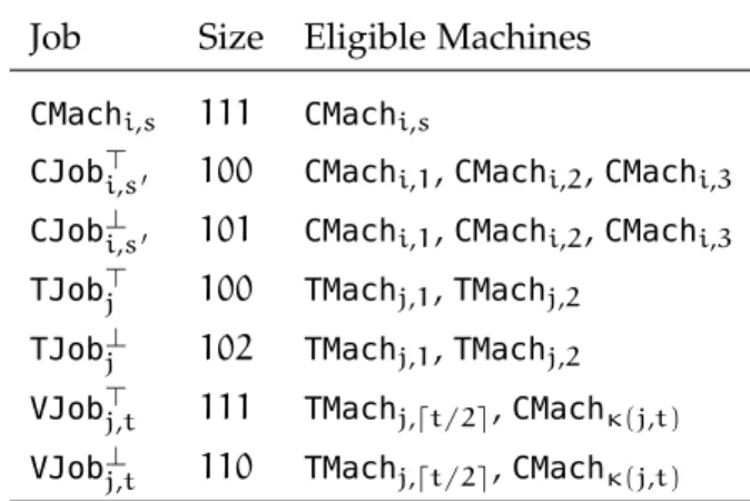
s i m p l i f i c at i o n o f t h e i n p u t. We construct a simplified in-stance ¯Iwith modified processing times ¯ptj. If a jobjhas a processing
time bigger than T for a machine typet∈[K], we set ¯ptj=∞. We call a job big (for machine typet) ifptj > ε2T and smallotherwise. We perform a geometric rounding step for each jobjwithptj<∞, that is, we set ¯ptj= (1+ε)xε2T withx=dlog1+ε(ptj/(ε2T))e.
l e m m a 3.5. If there is a schedule with makespan at most T forI, then the same schedule has makespan at most(1+ε)T for instance¯I; and any schedule for instance¯Ican be turned into a schedule forIwithout increase in the makespan.
We will search for a schedule with makespan ¯T = (1+ε)T for the rounded instance ¯I.
We establish some notation for the rounded instance. For any rounded processing timep, we denote the set of jobsj with ¯ptj =p by Jt(p). Moreover, for each machine type t, let St and Bt be the sets of small and big rounded processing times. Obviously, we have
|St|+|Bt| 6 n. Furthermore, |Bt| is bounded by a constant: Let N be such that (1+ε)Nε2T is the biggest rounded processing time for all machine types. Then we have (1+ε)N−1ε2T 6 T and therefore
|Bt|6N6log(1/ε2)/log(1+ε) +161/εlog(1/ε2) +1(usingε61).
m i l p. For any set of processing times P, we call the P-indexed vectors of non-negative integers ZP
>0 configurations (for P). The size Λ(C) of configuration C is given by Pp∈PCpp. For each t ∈ [K], we consider the setCt(T¯)of configurationsCfor the big processing times Bt and with Λ(C) 6 T¯. Given a schedule σ, we say that a machine i of type t obeys a configuration C if the number of big jobs with processing timepthatσassigns to iis exactlyCpfor each
p ∈ Bt. Since the processing times in Bt are bigger than ε2T, we havePp∈BtCp61/ε
2 for eachC∈C
t(T¯). Therefore, the number of distinct configurations in Ct(T¯)can be bounded by:
(1/ε2+1)N <(1/ε2+1)1/εlog(1/ε2)+1
=2log(1/ε2+1)1/εlog(1/ε2)+1 ∈2O(1/εlog2 1/ε)
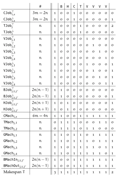
We define a mixed integer linear program MILP(T¯)in which con-figurations are chosen integrally and jobs are assigned fractionally to machine types. Note that we will call a solution of a MILP integral if both the integral and fractional variables have integral values. We introduce variables zC,t ∈ Z>0 for each machine type t ∈ [K] and configurationC ∈Ct(T¯), andxj,t >0for each machine type t∈[K] and jobj∈J. For ¯ptj=∞, we setxj,t =0. Besides this, the MILP has the following constraints:
X C∈Ct(T¯) zC,t=mt ∀t∈[K] (3.1) X t∈[K] xj,t=1 ∀j∈J (3.2)
3.2 b a s i c e p ta s 21 X j∈Jt(p) xj,t6 X C∈Ct(T¯) CpzC,t ∀t∈[K],p∈Bt (3.3) X C∈Ct(T¯) Λ(C)zC,t+ X p∈St p X j∈Jt(p) xj,t 6mtT¯ ∀t∈[K] (3.4) Because of Constraint (3.1), the number of chosen configurations for each machine type equals the number of machines of this type. Due to Constraint (3.2), the variablesxj,t encode the fractional assignment of jobs to machine types. Moreover, for each machine type, it is ensured with Constraint (3.3) that the summed up number of big jobs of each size is at most the number of big jobs that are used in the chosen configurations for the respective machine type. Lastly, (3.4) guarantees that the overall processing time of the configurations and small jobs assigned to a machine type does not exceed the areamtT¯. It is easy to see that the MILP models a relaxed version of the problem:
l e m m a 3.6. If there is schedule with makespanT¯, then there is a feasible (integral) solution ofMILP(T¯); and if there is a feasible integral solution for MILP(T¯), then there is a schedule with makespan at mostT¯ +ε2T.
Proof. Letσbe a schedule with makespan ¯T. Each machine of type
t obeys exactly one configuration fromCt(T¯), and we set zC,t to be the number of machines of type t that obey C with respect to σ. Furthermore, for a jobj∗let t∗ be the type of machineσ(j∗). We set
xj∗,t∗ =1andxj∗,t =0fort6=t∗. It is easy to check that all conditions
are fulfilled.
Now, let(zC,t,xj,t)be an integral solution of MILP(T¯). Using (3.2), we can assign the jobs to distinct machine types based on thex vari-ables. Thezvariables can be used to assign configurations to machines such that each machine receives exactly one configuration (utilizing (3.1)). Based on these configurations, we can create slots for the big jobs, and, for each typet, we can successively assign all of the big jobs assigned to this type to slots of the size of their processing time be-cause of (3.3). Now, for each type, we can iterate through the machines and greedily assign small jobs. When the makespan ¯T is exceeded due to some job, we stop assigning to the current machine and continue with the next. Because of (3.4), all small jobs can be assigned in this fashion. Since the small jobs have size at most ε2T, we get a schedule with makespan at most ¯T+ε2T.
We haveK2O(1/εlog2 1/ε) integral variables, i.e., a constant number.
Therefore, MILP(T¯)can be solved in polynomial time with the follow-ing classical result due to Lenstra [88] and Kannan [89]:
t h e o r e m 3.7: A mixed integer linear program with d integral variables and encoding sizes can be solved in timedO(d)poly(s).
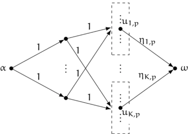
r o u n d i n g. In this paragraph, we describe how a feasible solution (zC,t,xj,t) for MILP(T¯) can be transformed into an integral feasible
α ... 1 1 .. . .. . .. . .. . .. . 1 1 1 1 ω η1,p ηK,p u1,p uK,p
Figure3.1: The flow network used for the rounding of the fractional variables.
solution (z¯C,t, ¯xj,t) for MILP(T¯ +εT+ε2T), where the second MILP is defined using the same configurations but properly changed right hand side. This is achieved via a flow network utilizing flow integrality.
For any (small or big) processing timep, letηt,p=dPj∈J
t(p)xj,te
be the rounded up (fractional) number of jobs with processing timep
that are assigned to machine typet. Note that for big job sizesp∈Bt, we have ηt,p 6 PC∈C
t(T¯)CpzC,t because of (3.3) and because the
right hand side is an integer.
Now, we describe the flow networkG= (V,E) with sourceαand sinkω. For each jobj ∈J, there is a job nodevj and an edge(α,vj) with capacity 1 connecting the source and the job node. Moreover, for each machine type tand processing time p∈Bt∪St, we have a processing time nodeut,p. The processing time nodes are connected to the sink via edges(ut,p,ω)with capacityηt,p. Lastly, for each jobj and machine type twith ¯pt,j <∞, we have an edge(vj,ut, ¯pt,j) with capacity1connecting the job node with the corresponding processing time nodes. We outline the construction in Figure3.1. Obviously we have|V|6(K+1)n+2and|E|6(2K+1)n.
l e m m a 3.8. Ghas a maximum flowfwith value|f|=n.
Proof. Since the outgoing edges fromαhave summed up capacityn,n
is a trivial upper bound for the maximum flow. The solution(zC,t,xj,t) for MILP(T¯) can be used to design a flowfwith value nby setting
f((α,vj)) = 1,f((vj,ut, ¯pt,j)) = xj,t andf((ut,y,ω)) =
P
j∈Jt(y)xj,t. It
is easy to check that fis indeed a feasible flow with valuen.
Using the Ford-Fulkerson algorithm, an integral maximum flow
f∗ can be found in time O(|E||f∗|) = O(Kn2). Due to flow conserva-tion, for each job j, there is exactly one machine type t∗ such that
f((vj,ut∗, ¯p
t∗,j)) =1, and we set ¯xj,t∗ =1and ¯xj,t =0fort6=t
∗
. More-over, we set ¯zC,t =zC,t. Obviously,(z¯C,t, ¯xj,t)satisfies (3.1) and (3.2). Furthermore, (3.3) is fulfilled because of the capacities and because
3.3 b e t t e r r u n n i n g t i m e 23
ηt,p 6
P
C∈Ct(T¯)CpzC,t for big job sizes p. Due to the geometric
rounding and the convergence of the geometric series, we have: X p∈St p6ε2T ∞ X i=0 (1+ε)−i=ε2T1+ε ε
This together withPj∈Jt(p)x¯j,t 6ηt,p<
P j∈Jt(p)xj,t+1yields: X p∈St p X j∈Jt(p) ¯ xj,t < X p∈St p X j∈Jt(p) xj,t+ X p∈St p < X p∈St p X j∈Jt(p) xj,t+ε2T 1+ε ε Hence: X C∈Ct(T¯) Λ(C)z¯C,t+ X p∈St p X j∈Jt(p) ¯ xj,t < mt(T¯ +εT+ε2T)
Therefore (3.4) is fulfilled as well.
a na ly s i s. The solution found for MILP(T¯) can be turned into an integral solution for MILP(T¯ +εT+ε2T). Like described in the proof of Lemma3.6this can easily be turned into a schedule with makespan
¯
T +εT+ε2T+ε2T 6(1+4ε)T. It is easy to see that the running time of the algorithm by Lenstra and Kannan (see Theorem3.7) dominates the overall running time. Since MILP(T¯)hasO(K/εlog1/ε+n)many constraints, Kn fractional and K2O(1/εlog2 1/ε) integral variables, the
running time of the algorithm can be bounded by: (K2O(1/εlog2 1/ε))O(K2O(1/εlog2 1/ε))
poly((K/εlog1/ε)|I|) = 2K2O(1/εlog2 1/ε)poly(|I|)
3.3 b e t t e r r u n n i n g t i m e
We improve the running time of the algorithm using techniques that utilize results concerning the existence of solutions for integer linear programs (ILPs) with a certain simple structure. In a first step, we can reduce the running time to be only singly exponential in1/εwith a technique by Jansen [72]. Then we further improve the running time to the one claimed in Theorem3.1with a result by Jansen et al.[73]. Both techniques rely upon the following result about integer cones by Eisenbrandt and Shmonin [43]:
t h e o r e m 3.9: Let X ⊂ Zd be a finite set of integer vectors and let b ∈int-cone(X) = {Px∈Xλxx|λx ∈Z>0}. Then there is a subset
˜
X ⊆X such that b ∈ int-cone(X˜) and |X˜| 6 2dlog(4dM), with M = maxx∈Xkxk∞.
f i r s t i m p r ov e m e n t. For the first improvement of the running time, this theorem is used to show:
c o r o l l a r y 3.1 0. MILP(T¯)has a feasible solution where for each machine type as few as O(1/εlog21/ε) of the corresponding integer variables are non-zero.
We get the better running time by guessing the non-zero variables and removing all the others from the MILP. The number of possibilities of choosingO(1/εlog21/ε)elements out of a set of2O(1/εlog2 1/ε)
ele-ments can be bounded by2O(1/ε2log4 1/ε). Considering all the machine
types, we can bound the number of guesses by 2O(K/ε2log4 1/ε). The
running time of the algorithm by Lenstra and Kannan (see Theorem 3.7) withO(K/εlog21/ε)integer variables can be bounded by:
O(K/εlog21/ε)O(K/εlog2 1/ε)poly(|I|) =2O(Klog(K)1/εlog3 1/ε)poly(|I|)
This yields a running time of:
2O(Klog(K)1/ε2log4 1/ε)poly(|I|)
Proof of Corollary3.10. We consider the configuration ILP for schedul-ing on identical machines. Let m0 be a given number of machines,
P be a set of processing times with multiplicitieskp∈Z>0 for each
p∈P, and letC⊆ZP
>0 be some finite set of configurations forP. The configuration ILP form0,P,k= (kp)p∈P, andCis given by:
X C∈C CpyC =kp ∀p∈P (3.5) X C∈C yC =m0 (3.6) yC ∈Z>0 ∀C∈C (3.7)
The default case that we will consider most of the time is that C is given by a target makespan T that upper bounds the size of the configurations.
Let us assume we had a feasible solution(z˜C,t, ˜xj,t) for MILP(T¯). For each t∈ [K]and p∈ Bt, we set ˜kt,p =
P
C∈Ct(T¯)Cpz˜C,t. We fix
a machine type t. By setting yC = z˜C,t, we get a feasible solution for the configuration ILP given by mt, Bt, ˜kt and Ct(T¯). Theorem
3.9can be used to show the existence of a solution for the ILP with only a few non-zero variables: Let X be the set of column vectors corresponding to the left hand side of the ILP and bbe the vector corresponding to the right hand side. Thenb∈int-cone(X)holds and Theorem3.9yields that there is a subset ˜XofXwith cardinality at most
2(|Bt|+1)log(4(|Bt|+1)1/ε2) ∈O(1/εlog21/ε) andb ∈int-cone(X˜). Therefore, there is a solution(y˘C) for the ILP with O(1/εlog21/ε) many non-zero variables. If we set ˘zC,t = y˘C and ˘xj,t = x˜j,t and perform corresponding steps for each machine type, we get a solution