THE RESEARCH INSTITUTE OF INDUSTRIAL ECONOMICS
Working Paper No. 570, 2002
Cross-Border Acquisitions and Greenfield Entry
by Pehr-Johan Norbäck and Lars Persson
IUI, The Research Institute of Industrial Economics P.O. Box 5501
Cross-Border Acquistions and Greenfield Entry
Pehr-Johan Norbäck
∗The Research Institute of Industrial Economics
Lars Persson
The Research Institute of Industrial Economics and CEPR
January 10, 2002
Abstract
We investigate the interaction between cross-border acquisitions and greenfield entry in a multi-firm setting. It is shown that the net profits of the acquirer may decrease when the acquisition gives the acquirer a strong position in the product market, relative to greenfield entrants. The reason is that the price of the assets increases more than the acquirer’s profit, due to strategic interaction effects in the product market. The paper also provides an explanation why MNEs entering a new market by acquisitions may make a lower profit than MNEs entering greenfield. A greenfield entrant faces the risk of not being able to successfully locate production due to the lack of knowledge of characteristics of the local market. The bidding competition between the MNEs for being successfully located in the market then drives up the acquisition price to such a level that being a successful greenfield entrant is, ex post, more profitable.
Keywords: Investment Liberalization, FDI, Mergers & Acquisitions. JEL classification: F0, F2, L1
∗We are grateful for helpful discussions with Jonas Björnerstedt, S-O Fridolfsson, Chiara Fumagalli,
Mattias Ganslandt and Monika Schnitzer, and participants at IUI seminars and the 2001 SAET con-ference in Ischia. Financial support from the Marianne and Marcus Wallenberg Foundation, and Tom Hedelius’ and Jan Wallander’s Research Foundations, is gratefully acknowledged. Email: [email protected].
1. Introduction
Multinational Enterprises (MNEs) can use two types of business strategies to conduct foreign direct investment (FDI); they can either acquire (or merge with) a firm in the host country or invest greenfield, i.e. set up a new plant in the host country.
When will the MNEs prefer acquisitions to greenfield investment? Several factors have been argued to be important for explaining why MNEs prefer to grow via M&As rather than through organic growth: the quest for strategic assets, such as brand names, the possessions of local permits or distribution networks and patents. Moreover, when the time to market is vital, the takeover of an existingfirm with an established distribution system is preferable to developing a new local distribution and marketing organization.1
All these motivations seem build on the fact that the acquirer gains a strong position in the product market by its acquisition. In order to capture this aspect, the domestic assets will be said to be strategically valuable when giving the acquirer a strong position
in the product market, relative to greenfield entrants.
We present a model where we indeed show that a high strategic value of the domestic assets is conducive to acquisitions. However, while acquisition entry is associated with a high strategic value of the domestic assets, we also show that such acquisitions might have low profitability: the net profits of the acquirer may decrease, the more strategically valuable the domestic assets are. In the model, a domestic firm is initially located in the domestic market in country H. There are also several MNEs located in the world market. The domestic market will now be exposed to international competition. The interaction takes place in three stages. In the first stage, the MNEs might acquire the domesticfirm’s assets. In the second stage, MNEs have the option of investing greenfield in new assets in country H. Finally, in the third stage,firms compete in oligopoly fashion in country H.
The result that the net profits of the acquirer, i.e. the product market profit net
1See World Investment Report (WIR) 2000 and its reference to different studies of cross-border
of acquisition price, may decrease in the strategic value of the domestic assets seems counterintuitive at first sight, since the domesticfirm’s assets are then more valuable to the MNEs when acquired. However, this result is intuitive, when taking into account how the level of strategic value of the domestic assets affects the acquisition price. The price of the assets is a non-acquiring MNE’s willingness to pay, which consist of two profit terms: the profit for this firm if it would instead obtain the domesticfirm’s assets net of the profit when not buying. It then follows that thefirst profit term increases to exactly the same extent as that of the acquirer from an increase in the strategic value of the domestic assets, and will thus off-set the acquirer’s profit increase. Moreover, the second profit term will decrease, the more strategically valuable the domestic assets are, since the non-acquirer will then face a stronger competitor in the product market. This implies that the willingness to pay increases further for the non-acquirer. Consequently, the acquisition price increases more than the acquirer’s product market profit when the domestic assets become more strategically valuable.
In the literature on MNEs2, it has also been argued that one of the main benefits from
acquiring a local competitor instead of entering greenfield is that the acquisition helps the firm avoid risks due to lack of knowledge of the specific characteristics of the local market. Moreover, there may be several MNEs competing to enter the market, all of which may not be able to make a profitable entry, thereby making greenfield investment risky. By entering by a M&A, an MNE avoids the risk of unsuccessful greenfield entry. However, we show that the “extra” value of avoiding this risk is competed away in the bidding competition over the domestic (target) firm’s assets. The price of the domestic firm’s assets will be determined such that the net profit of the acquirer is the expected value of being a successful greenfield entrant with a certain probability and an unsuccessful entrant with a certain probability. The bidding competition over being successfully located in the market with certainty thus drives up the acquisition price to such a level that being a greenfield entrant ex post is more profitable. We thus show that MNEs entering a new market by M&As may make a lower profit than MNEs entering greenfield.
The selling of the failing South Korean car-producer Daewoo in 2000, where FORD acquired Daewoo in competition with Daimler-Chrysler and Hyundai and GM and FIAT, provides an example of the insights this paper may offer. According to Business Week (January 2000), an acquisition of Daewoo would (i) provide the acquiring firm with strategically valuable assets (instant command of 1/3 of the South Korean market, the second largest market in Asia), and (ii) secure and facilitate large scale entry into the Asian market.3 In this situation, FORD apparently paid a high price for the South
Korean firm as indicated by the following quote from the Economist (2000): Insiders admit that FORD was willing to pay well over the odds for the South Korean company
because of the strength it would thereby acquire in Asia. FORD actually paid such a
high price that, in September 2000, it abandoned its bid for Daewoo, when the revealed problems with Daewoo’s assets turned out to be worse than FORD had anticipated. (Business Week October, 2000). The apparently low profitability of FORD’s bid then seems to stem from a combination of - on the one hand - a high acquisition price triggered by bidding competition over strategically valuable assets and - on the other hand - underestimating Daewoo’s debts and liabilities.4
The strategic motive for paying a high price for strategically important assets also seems to have been important in the bidding competition over Banco do Estado de Sao Paulo (Banespa), the seventh-largest bank in Brazil. In November 2000, Banco Santander Central Hispanio (BSCH) won a controlling minority stake in Banespa, in competition with several other large banks, including its Spanish rival Banco Bilbao Vizcaya Argentaria (BBVA). According to Business Week (April 23, 2001): “It cost an astronomical $3.55 billion, but it put BSCH back on top” (before BBVA - authors comment). The assets of Banespa were considered strategically valuable, as indicated
3For FORD, the later motivation seemed very important as indicated by the following quote from
the Economist (2000), commenting on FORD’s vulnerable situation as a non-acquirer: there is nothing left for Ford to acquire, leaving organic growth as its only hope.
4FORD offered to pay $6.9 billion. To our knowledge the bids from the other bidders were not
revealed. However, recently GM paid $400m for a 57% stake in Daewoo. (Financial Times, October, 2001).
by the following quote ”Anyone who can add Banespa to their existing structure will take a gigantic leap forward,” says Elio Duarte, director of institutional relations at the Brazilian subsidiary of Britain’s HSBC Holdings PLC, one of the nine banks qualified to take part in the auction.” (Business Week, November 20, 2000). According to Business Week (November 20, 2000), this means that ”...bidders will pay a premium not just to get their hands on Banespa but also to stop rivals from doing so.”
The related theoretical literature on FDI and MNEs is surveyed in Markusen (1995). This literature does not explicitly address the question of whether entry into a foreign market is greenfield or through the acquisition of assets already in the market, or both. This issue is at focus in our study, however.5
There is also a small theoretical literature addressing aspects of cross-border mergers in international oligopoly markets.6 However, the equilibrium acquisition price, which is in focus in our study, is not determined in those studies.
The model is spelled out in Section 2. In Section 3, we derive the equilibrium market structure. Section 4 concludes. Finally, most proofs appear in the Appendix.
2. The Model
Consider a countryH, where the market has previously been served by a single domestic firm, denoted d, possessing one unit of domestic assets, denoted ¯k. This market will now be exposed to international competition.7 There are several different reasons why the market is exposed to international competition at this stage, but not previously. For instance, the country might be investment liberalizing, the expansion might be a natural step in the life cycle of a product8 or stem from increasing local demand, or 5See Görg (1997) and Das and Sengupta (2001) for papers addressing the choice of entry mode.
However, these papers abstract from the competition between MNEs, which is at focus in our study.
6This literature includes papers by, for example, Bjorvatn (2001), Head and Reis (1997) and Horn
and Persson (2001).
7It is of no consequence whether the market was previously open to imports.
8Caves (1996, p.58) argues that many MNEs cannot expand quickly due to constraints of growth.
the administrative costs of cross-border acquisitions and greenfield entry may have been reduced in the globalization process.
We assume that there are M >1 symmetric MNEs in the world market. The MNEs did initially not have any assets in Country H, but might now invest. The interaction takes place in three stages. In the first stage, the MNEs might acquire the domestic firm’s assets. In the second stage, MNEs have the option to invest greenfield in new assets in country H. Finally, in the third stage, firms compete in oligopoly fashion in country H.9
The next sections describe the product market interaction, the greenfield investment game, and the acquisition game.
2.1. Stage three: product market interaction
The profits in the industry will depend on the distribution of asset ownership. Due to symmetry, we need only to distinguish between two types of ownership structures: (i) the one where the domestic assets are sold to one of the MNEs, denotedkm, and (ii) the one where the domestic assets remain in the hands of the domestic owner, denotedkd.
Vectors km andkd are defined as follows:
km ≡ km(α, Nm)≡(0,αk, k¯ G, kG,..., kG, Nm 0, ...,0 M−Nm−1 ), α>0 (2.1) kd ≡ kd(1, Nd)≡(¯k, kG, kG,..., kG, Nd 0, ...,0 M−Nd ). (2.2)
Thefirst entry in each vector shows the asset ownership of the domesticfirm, the second entry is the asset ownership of the, potentially, acquiring MNE. The parameter α > 0 captures that an MNE and the domestic firm may differ in how efficiently they can use the assets ¯k. We shall discuss the parameter α in detail below. The remaining entries show the asset ownership of the non-acquiring MNEs, being either greenfield entrants
9The choice of timing between the acquisition and the greenfield investment is not obvious in a
general setting. In this particular application, however, it seems natural for the acquisition decision to be made before the greenfield decision, since the assets for sale already exist in the market and entering greenfield requires the construction of a new plant, which is usually time consuming.
(having assets kG) or ”exporters”, i.e. non-investing MNEs (having assets kE ≡ 0). Under MNE ownership, there is one acquiring MNE and Nm non-acquiring MNEs that invest greenfield, whereasM−Nm
−1MNEs do not invest. Under domestic ownership, there are Nd MNEs investing greenfield andM −Nd MNEs that do not.
Under MNE ownership of the domestic assets k¯, we let πA(km) denote the reduced-form product market profit for the acquiring MNE, πG(km) the corresponding profit for a non-acquiring MNE as a greenfield entrant, and πE(km)the corresponding profit for a non-acquiring MNE as exporter (i.e. a non-investing MNE). Under domestic ownership of the assets¯k, MNEs are either greenfield entrants or exporters, with profitsπG(kd)and
πE(kd), respectively.The corresponding profit for the domesticfirm under the respective ownership structures are πd(kl), l ={d,m}.
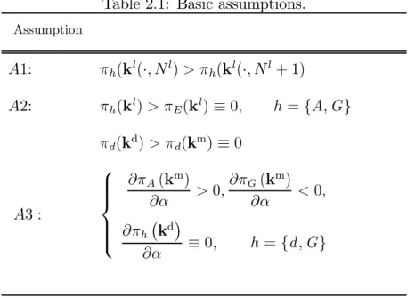
We make the following assumptions about profits in the product market as summa-rized by table 2.1:
Table 2.1: Basic assumptions. Assumption A1: πh(kl(·, Nl)>πh(kl(·, Nl+ 1) A2: πh(kl)>πE(kl)≡0, h={A,G} πd(kd)>πd(km)≡0 A3 : ∂πA(km) ∂α >0, ∂πG(km) ∂α <0, ∂πh kd ∂α ≡0, h={d,G}
Assumption A1 states that the product market profit for all types of firms decreases in the number of greenfield entrants, Nl. We describe greenfield entry in detail in the next section.
H. This assumption then forms the basic motive for FDI in terms of acquisition or greenfield entry, stemming from trade cost avoidance or lower factor costs. To facilitate readability, but with no loss of generality, we normalize such thatπE(kl)≡0, i.e. export profits for MNEs, are set to zero.10 Moreover, we also assume that the domestic firm will not make any product market profit without its assets,πd(km) = 0.
The local assets¯kmay be used differently under domestic and foreign ownership. As-sumption 3 then states that an increase inthe strategic value,α, increases the acquirer’s profit, whereas the market profit for a non-acquirer (i.e. greenfield investor) decreases. The size of these effects depends on the strength of complementarities between MNEs´ firm-specific assets and the domestic assets. For example, the combination of an MNE’s strong brand name and the acquired firm´s knowledge of the market or strength in dis-tribution may provide the acquiring MNE with a strong market position. If the brand name of the domestic assets are locally very strong, the strategic value of the assets will also be high. Or, if the domestic assets are sold at an early stage, the acquirer may gain a strong first-mover advantage, building up a dominant position in the product market.11
This set-up and these assumptions are compatible with several different oligopoly models. For example, Farell and Shapiro (1996) study changes in exogenous assets ownership, assuming the product market competition to be Cournot. Under general assumptions on demand and costs, they show that an increase in capital for a firm (i) increases this firm’s profit, while (ii) decreasing the profits of its competitors. Since
kA=αk¯, an increase inα corresponds to an increase in effective asset ownership by the acquiring MNE, the Farrell and Shapiro model (1996) is compatible with this set-up. Moreover, using a quantity-setting conjectural variation oligopoly model under a set of
10It can shown that all results in this paper can be derived without this normalization, allowing for
the service or good produced by this industry to be either tradable or non-tradable.
11As a specific example, in the retail industry, MNEs acquire local retail chains and combine their
advantages of global sourcing with the advantages of the established distribution network. As Greenfield entry does not have this advantage, and it takes more time to build local assets, an acquiring MNE is at an advantage. While having the initial possession over the distribution network, a domesticfirm lacks the advantage of global sourcing.
stability criteria, Dixit (1986) shows that a change, which is prima facie favorable to a firm, as is an increase in capital (α), reduces the profits of all other firms.
2.2. Stage two: Greenfield investments
At this stage, MNEs that did not enter the market through the acquisition of firm d, can enter by undertaking a greenfield investment at a fixed cost, G.12 To simplify the
analysis, we assume that investments into greenfield assets kG are ”lumpy”, i.e. they come in discrete assets or plants and that the domestic firm does not find it profitable to invest in this stage due to, for instance, financial or managerial restrictions.
Assumption A2 states that there are locational advantages for MNEs from producing in country H. We use two different ways of determining the number of MNEs which take advantage of such business opportunities by investing greenfield, Nl:
(i) Greenfield entry might be risky due to lack of knowledge of the specific character-istics of the local market. In the literature on MNEs, it is argued that one of the main benefits of acquiring a local competitor instead of entering greenfield is the avoidance of such risks.13 To this end, we assume that there is an exogenous individual risk of failure in greenfield entry.14 We denote the probability of successful entry asPl = P. Nl is then simply the MNEs drawn as successful in the greenfield stage.
(ii) Alternatively, all MNEs may not face profitable greenfield entry due to insufficient demand. To determine the number of entrants in this case, we assume the pool of potential entrants to be ordered in sequence, where each possible ordering can be drawn with equal probability.15 Entry then takes place until the lastfirm cannot cover its entry
costG, that is,Nl must fulfillπ
G(kl(·, Nl)>G andπG(kl(·, Nl+1)≤G. The probability
12There is then implicitly assumed to be a minimum efficient plant scale, which is not too small
relative to market demand.
13See Caves (1996).
14Consequently, we assume that there is no correlation between the probability of successful greenfield
entry for different MNEs.
of successful greenfield entryPl is then: Pl = Nm M−1 if l =m Nd M if l =d. (2.3)
Note that in this case, an MNE’s probability of greenfield entry may not be the same under a different ownership of the domestic assets: First, the number of MNEs competing for greenfield entry is different. In addition, the number of profitable greenfield entrants
Nl may not be the same. This follows directly from Assumption A3, where it is assumed that the product market profits for greenfield entrants differ under different ownerships of the domestic assets.16
2.3. Stage one: the acquisition game
To focus on the bidding competition among MNEs as the determinant of the equilibrium buyer, we assume that MNEs post bids for the domesticfirm, which thatfirm may accept or reject.17 More specifically, the acquisition process is depicted as an auction whereM
MNEs simultaneously post bids and the domesticfirm then either accepts or rejects these bids.18 Each MNEi announces a bid,b
i, for the domesticfirm. b= (b1, b2, ..., bM)∈RM
16What is important for most of our results is that the expected profit for a firm participating in
the greenfield investment game is non-negative for all parameter values and positive for some. The results in the paper hold if the investment game can be modeled as simultaneous game and solved for Nash equilibria in pure strategies, where each equilibrium is assumed to have equal probability. In a general simultaneous entry approach, there might be over as well as underinvestment, however (Dixit and Shapiro (1986)). Another approach is to include a pre-entry period, wherefirms can use irreversible commitments to convert the game into a sequential one. Nti (2000) then shows that in such an approach, the expected net profit of participating in the investment game is positive.
17The main results of the paper would hold if there were initially more than one domesticfirm in the
market. However, several other aspects would then have to be taken care of, such as the possibility of domestic mergers, timing of the selling of the different domestic firms, etc., and the analysis of these issues is outside the scope of this paper.
18The main result in the acquisition game would also hold in a setting where the domesticfirm states
an asking price simultaneously with the MNEs’ bids. There will be multiple equilibria, not present in this set-up, for some parameter values in such a setting, however.
is the vector of these bids. Following the announcement of b, the domestic firm may be sold to one of the MNEs at the bid price or remain in the ownership of firmd. If more than one bid is accepted, the bidder with the highest bid obtains the domestic assets. If there is more than one MNE with such a bid, each such MNE obtains the assets with equal probability. The acquisition is solved for Nash equilibria in undominated pure strategies.19
It is assumed that firm d cannot make a bid for the MNEs. This assumption might be motivated by the domestic owner being financially weaker or lacking the competence to efficiently run the larger business. Moreover, it is assumed that MNEs cannot make bids on each other’s firms. This assumption might be supported in a full merger model in two basic ways. One is to assume that the profit of a merged entity is small enough to imply that no merger takes place between the MNEs.20 The second possibility would be to assume that mergers between MNEs would not be permitted by the competition authorities.
We now turn to thefirms’ valuations of the domesticfirm’s assets¯k. There are three different valuations which need to be considered:
vmimj is the value for MNEi of obtainingk¯, when MNE j would otherwise obtaink¯. Using symmetry among MNEs, we will suppress the subindices and simply write vmm. The first term shows the profit when possessing ¯k. The second term is the expected profit when a rival MNE obtains ¯k,in which case greenfield entry in stage 2 takes place with probability Pm.
vmm=πA(km)−Pm[πG(km)−G] (2.4)
vmd is the value for MNE i of obtaining k¯ when the domestic firm would otherwise keep them. The expected profit for MNE i when not obtaining assets ¯k is different in
19There is a smallest amount, ε, chosen such that all inequalities are preserved if ε is added or
subtracted.
20For instance, it has been shown by Kamien and Zang (1990) that the hold up problem in merger
formation might lead to no merger taking place in equilibrium, if the initial number of firms is suffi -ciently large. Moreover, mergers might be non profitable since the costs associated with mergers can be substantial, for example due to problems of melting together different company cultures.
this case, for two reasons. First, when the¯k assets are in the hands of the domesticfirm, they might be used differently from when in the hands of an MNE. This implies that the profits as a greenfield entrant will typically be different. Second, as previously discussed in section 2.2, the probability of succeeding with greenfield entry may also be affected by a change in the ownership of the domestic assets.
vmd =πA(km)−Pd πG(kd)−G (2.5)
vd is the value for the domestic firm of obtaining k¯. Consequently, since we have assumed that πd(km) = 0:
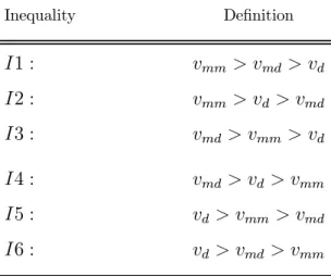
vd =πd(kd). (2.6) Thefirms’ bidding behavior is dependent on the relation between their own valuation of obtaining assets k¯ and all other firms’ valuations of obtaining these assets. Since MNEs are symmetric, valuations vmm, vmd and vd can be ordered in six different ways, as shown in table 2.2. As will be shown in the analysis below, these inequalities are useful for illustrating the results.
Table 2.2: Orderings of valuations
Inequality Definition I1 : vmm> vmd> vd I2 : vmm> vd> vmd I3 : vmd > vmm> vd I4 : vmd > vd> vmm I5 : vd> vmm > vmd I6 : vd> vmd> vmm
3. The equilibrium ownership structure
We are now set to derive the equilibrium ownership structure (EOS), the acquisition price, A, and the net profit for each type of firm in the international oligopoly laid out above. To this end, we need some further notation. As stated earlier, in equilibrium, three types of firms can exist: (i) The net profit of the MNE that has acquired the k¯
assets is denoted ΠA and consists of product market profits net of the acquisition price, i.e. ΠA(km) = π
A(km)−A, (ii) MNEs that have invested greenfield. ΠG denotes this firm’s net profit, i.e. ΠG(km) =π
G(km)−GandΠG(kd) = πG(kd)−G when the domestic assets are under MNE and domestic ownership, respectively and (iii) the domestic firm. Πd denotes the domesticfirm’s net profit, i.e. Πd(kd) = π
d(kd), if assets¯k remain in d’s ownership and Πd(km) =
A otherwise. We can then state the following lemma.
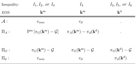
Lemma 1. The equilibrium ownership structure (EOS), acquisition price and net profit for each type of firm are described in table 3.1:
Proof. See the Appendix.
Table 3.1: Equilibrium ownership, acquisition price and net profits. Inequality: I1, I2,or I3 I4 I2, I5,or I6 EOS: km km kd A: vmm vd . ΠA: Pm[π G(km)−G] πA(km)−πd(kd) . ΠG : πG(km)−G πG(km)−G πG(kd)−G Πd: vmm vd πd(kd)
Lemma 1 shows that when one of the inequalities I1, I3, or I4 holds, ¯k is obtained by one of the MNEs. Under I1 and I3, the acquiring MNE pays the acquisition price
A=vmm, andA =vdunder I4. When I5 orI6 holds, the domesticfirm keeps its assets. WhenI2 holds, there exist multiple equilibria.21
Lemma 1 has some noteworthy implications. For instance, Caves (1996) argues that the acquisition price will be high, due to equity share holder competition, which implies that the MNE must at least pay the maximum value of the firm in the hands of local management, i.e. vd. Lemma 1 shows that the acquisition price will be the maximum of vmm andvd, since not only shareholders but also other MNEs compete to acquire the assets.
Moreover, the main motivations for MNEs to acquire the domestic firm’s assets is that ownership of these assets allows an early entry into the market or give access to proprietary assets. Increasing the strategic value of the domestic assets, increasingα, will increase the profit in the product market for the acquirer, relative to greenfield MNEs. This makes the bidding competition between the MNEs tougher and drives up the MNEs’ valuations of the domestic assets. This, in turn, will lead to a foreign acquisition of the domestic assets, as shown by the following Proposition:
Proposition 1. Given that the strategic value of the domestic assets is sufficiently
high, α>α∗, the equilibrium asset ownership structure is km.
Proof. See the Appendix.
However, while high strategic value is conducive to foreign acquisitions, high strategic value is not necessarily associated with high profitability as shown in the next section.
3.1. Profitability and the strategic value of the domestic assets
When bargaining between an MNE and a domestic seller takes place in isolation, acqui-sition entry should become more profitable as compared to greenfield entry, the more strategically valuable the domestic assets are. The reason being that both parties gain when the total surplus increases in most bargaining models. However, when there are
21 An equilibrium wherefirmd keeps the assets and no MNE posts a bid abovev
d. There is also an equilibrium where one of the MNEs obtains the assets at a price vmm−ε and another MNE posts the second highest bid atvmm−2ε.
several potential buyers of the domesticfirm’s assets, the net profits of the acquirer may decrease as illustrated by the following Proposition:
Proposition 2. When several MNEs are potential buyers of the domesticfirm’s assets, the net profits of all types of MNEs, including the acquirer, may decrease, the more strategically valuable the domestic assets are.
To explain this result, we explore how the net-profit of the acquiring MNE, ΠA, changes from an increase in parameterα when I1, I2 or I3 holds. In these cases, bidding competition among the MNEs over the domesticfirm’s assets is more intense, since the value of preventing other MNEs from obtaining the domestic assets is high.
To proceed, let E [ΠN A] denote the expected profit (omitting the asset-ownership vector km as an argument), at the beginning of period 2 for an MNE not acquiring the domesticfirm’s assets. The net profit of the acquiring MNE can then be written:
ΠA = πA(km)−A (3.1) = πA(km)−[πA(km)−E [ΠN A]] (3.2) = E [ΠN A]
≡ Pm[πG(km)−G] (3.3) First, note that any increase in profit due to an increased strategic value of the domestic assets k¯ for the buyer is off-set. The reason is that the price of the assets is determined by a non-acquiring MNE’s willingness to pay, which, in turn, is determined by the two terms in the bracketed expression in (3.2). The first term is the profit for the non-acquiring MNE, if this firm were to obtain k¯. This will increase to exactly the same extent as the acquirer’s profit and will thus off-set the acquirer’s profit increase. Hence, the change in net profit for the acquirer from a change in strategic value of the domestic assets is then completely determined by the change in profit of the non-acquirer when not buying. This profit, E [ΠN A], is the second term in the bracketed expression in (3.2), and is written out in (3.3). If E [ΠN A] decreases (increases) due to increase in
the strategic value of the domestic assets, the net profit of the acquirer, ΠA, will then decrease (increase). Three effects will determine how this profit changes whenαchanges.
3.1.1. Strategic value and product market effects
Let us first assume that the risk of failure in greenfield investment does not depend on
α. This would correspond to case (i) version of the greenfield game in Section 2.2 or to the situation where the change in α is so small that the number of greenfield entrants is not affected in version (ii). We can then treat the probability of successful greenfield entry, Pm, as exogenous. It then follows that there is a product-market effect on the non-acquirer’s profit from an increase in strategic value. This product-market effect is negative since non-acquiring MNEs, that is, greenfield entrants, now face a stronger competitor:
∂E [ΠN A]
∂α = P
m∂πG(km)
∂α <0, (3.4)
where we have used E [ΠN A]≡Pm[πG(km)−G]from (3.3) and ∂πG(k m)
∂α <0 by Assump-tion A3.
Any benefits from acquiring the domestic firm’s assets are competed away in the bidding competition among potential buyers. The only thing left is any negative exter-nalities on rivals the acquired assets might generate, and these become stronger the more strategically valuable the domestic assets are.
3.1.2. Strategic value and entry effects
If the number of greenfield entrants Nm is affected by a change in α, there are two additional effects: The investment game value effect and the entry possibility effect.
Rewriting (3.3) into E [ΠN A] = PmΠG and taking into account that there is then a discrete change in the number of greenfield entrants Nm, we can write the sum of these
effects as:22
∆E [ΠN A] = Pm[ΠG(Nm+∆Nm)−ΠG(Nm)] +∆PmΠG(Nm+∆Nm) (3.5)
The investment game value effect, represented by the first term in (3.5), shows how
the profit of participating in the entry game is affected when the number of successful entrants changes. The entry possibility effect, as represented by the second term in (3.5), shows how the expected profit changes with the changed probability of successful greenfield entry. It follows from Assumption 3 that the stronger the acquiring MNE becomes in the product market competition, the less profitable is greenfield entry. The investment game value effect is then positive since from Assumption A1, the aggregate profit in the investment game increases when product market competition is weakened, due to a lower number of greenfield entrants. On the other hand, the entry possibility effect will be negative. The reason is that greenfield entry is less likely since the acquirer now being a stronger competitor.
In summary, if the probability of successful greenfield entry Pm is exogenous, the net profits of all types of MNEs, including the acquirer, decrease the more strategically valuable the domestic assets are.23 The reason is that any benefits from acquiring the domestic firm’s assets are competed away in the bidding competition among potential buyers. The only thing left is any negative externalities on rivals the acquired assets might generate, and these become stronger the more strategically valuable the domestic assets become. When the probability of successful greenfield entryPmdepends onα, we also need to take the two entry effects into account. It then follows that the net profits could increase as well as decrease when the domestic assets become more strategically valuable. This is also illustrated in a linear Cournot model in Appendix A.6 (see, figure A.1).
22We write net profits directly as a function of the number of greenfield entrants,Π(N). ∆Nmis the
change in the number of greenfield entrants and, from (2.3),∆Pm=∆Nm
M−1 is the corresponding change in the probability of greenfield entry.
23Note that the acquirer benefits if I4 holds, since an increase inα then implies that the acquirer’s
3.2. Profitability and limited greenfield possibilities
An MNE not entering by M&A faces the risk of not being able to successfully locate production in the market. We have provided two reasons why this might be the case: (i) Greenfield entry might be risky due to the lack of knowledge of the specific characteristics of the local market.24 (ii) There may be several MNEs competing to enter the market, all of which may not be able to make profitable entry.
Let us now compare the net profits for the different types of firms, given that the domestic assets are sold, i.e. I1, I2, I3 or I4 holds. We then have the following result:
Proposition 3. An MNE successfully entering greenfield makes at least as high a net profit as an MNE entering by acquisition.
Proof. See the Appendix.
Equilibrium acquisitions should be profitable relative to greenfield entry when bar-gaining between the acquiring MNE and the seller takes place in isolation, since the buying MNE would otherwise enter greenfield. But when there are several potential buyers for the domestic firm, the price of the domestic firm’s assets will be determined such that the non-acquirer (and the acquirer) is indifferent between acquiring and not acquiring.25 Consequently, the expected profit from entry by acquisition should equal the expected profit from greenfield entry. However, when there is a risk associated with greenfield entry, the ex post profit for the acquirer will be lower than the ex post profit for the successful greenfield entrant.
24One other possible interpretation of this situation is that each firm invests a fixed cost F when
participating in the investment game, for instance lobbying or marketing costs. Firms are then randomly drawn as successful over time. Afirm drawn as successful would then enter iffprofitable according to the entry conditions in the model. πG(kl)would then correspond to the profit for a successful entrant
andπE(kl)to the profit for an unsuccessful entrant. This implies that we can use our set-up as long as
the expected profit for a greenfield entrant is still non-negative.
25This is true under I1-I3, under I4 the expected profit for the acquirer is lower than the expected
3.3. Stockmarket value and cross-border acquisitions
In this section, we will make a couple of remarks on the implications for stock market value. Following the standard approach in the so-called event studies on M&A perfor-mance, we assume that the acquisition comes as a surprise for thefinancial markets.26 We
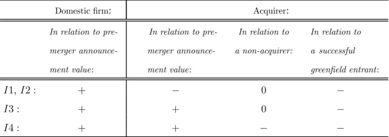
then show in table 3.2 how thefirms’ stock market values are affected by the acquisition.
Table 3.2: Change in stockmarket value. Domesticfirm: Acquirer: In relation to pre-merger announce-ment value: In relation to pre-merger announce-ment value: In relation to a non-acquirer: In relation to a successful
greenfield entrant:
I1,I2 : + − 0 −
I3 : + + 0 −
I4 : + + − −
Note : A formal proof is provided in Appendix A.5. Figures A2 and A3 provide an illustration for the results in the second column for a linear Cournot model .
The first column compares the stock market value of the target at the time of the announcement of the acquisition to its pre-merger announcement value. The bidding competition implies that the domestic firm will sell its assets at a higher price than its pre-merger value vd = πd(kd). Moreover, under I1, I2 or I3, the acquisition price is possibly substantiality higher since A =vmm > vd. Hence, the target firm’s share price increases when the acquisition is announced.27
26Fridolfsson and Stennek (1999) argue that the stockmarket, if being efficient, should anticipate the
merger, and the new information in the merger announcement is which firms are insiders and which are outsiders. Under this assumption they show that preemptive mergers could explain the empirical evidence that mergers reduce profits and raise share prices. The reason is that the profit decreases less for insiders than for outsiders.
27This seems consistent with empirical results from event studies on merger performance. The event
The effect on the acquirer is more involved, and depends on the reference point. In the second column, we compare the net-profits of the acquiring firm, ΠA(km), with its pre-merger announcement value, which is the expected net-profit of this firm, had no acquisition occurred, E ΠG(kd) = Pd πG(kd)−G . Under I3 or I4, an acquisition leads to an increase in net profits, and, consequently, to an increase in stock market value. However, more surprisingly, under I1 or I2, an acquisition lowers the net profit of the acquirer and reduces the stock market value of this firm. Recall from section 3.1 that a high strategic value of the domestic assets generates a high acquisition price, since the acquirer makes a high product market profit, while the product market profit as a non-acquirer is low. When I1 or I2 holds, the latter effect is so strong that the acquiring firm faces a lower net-profit as compared to a situation when no acquisition takes place.28
In column three, we compare the stock-market value of the acquirer to that of a non-acquirer.29 Since the bidding competition makes MNEs indifferent between buying and not buying, the stock market value of the acquirer relative to a non-acquirer remains unchanged when the acquisition is announced. Hence, while the acquirer’s stock market value may be reduced as a consequence of the acquisition, participating in the bidding competition is nevertheless consistent with profit maximization.30
Finally, we compare the acquirer’s profit to a greenfield entrant at the time when the greenfield uncertainty is resolved. From section 3.2, we have seen that when there is a risk associated with greenfield entry, the ex post profit for the acquirer,ΠA(km), will be lower than the ex post profit for the successful greenfield entrant, ΠG(km). Hence, the prices a few weeks before and after the event. The results from these studies are that the targetfirms’ shareholders benefit, and the buyingfirms’ shareholders break even. See Scherer and Ross (1990) and its references to empirical studies on M&A performance.
28In appendix A.6, we illustrate these results using a linear Cournot model (see,figures A.2 and A.3). 29We then compare the net-profits of the acquiringfirm,Π
A(km), with the expected net-profits of the
non-acquirer,E [ΠN A] = E [ΠG(km)] = Pm[πG(km)−G].
30Note also that under I4, all MNEs benefit from an acquisition. The acquirer bears the costs of
the acquisition, however. Therefore, the acquirer’s stock market value is reduced in relation to a non-acquirer.
stock market value of the acquirer relative to a greenfield entrant decrease. We can summarize:
Corollary 1. The stock market value of the domesticfirm increases when the acquisition is announced. The stock market value of the acquirer may increase or decrease.
4. Concluding discussion
In this paper, it has been shown that the bidding competition over the domestic target firm implies that there are no excess profits to be made in cross-border acquisitions when bidding firms are symmetric. We have also shown that this bidding competition implies that the domestic firm will sell its assets at a higher, and possibly substantiality higher, price than its reservation price. The empirical implication is then that the target firm’s shareholders benefit from the acquisition, which seems consistent with the existing empirical literature. The predictions for the acquirer are more involved. However, an interesting finding is that the share value of both the buyer and the non-buyer will decrease when a merger is announced if the domestic assets are sufficiently strategically important. This is due to the fact that the bidding competition is then sofierce that the firms involved would be better off not starting a bidding war.31
If there is a risk associated with greenfield entry our empirical prediction is that, in the long run, when the greenfield uncertainty is resolved, the share value of a successful greenfield entrant should perform better than the share value of the acquirer. To test this hypothesis, we would need to be able to distinguish between successful and unsuccessful non-acquirers. One possibility would be to use data from markets opened up by an investment liberalization. It should then be possible to identify the MNEs active in the industry: acquiring firms, greenfield entrants, exporters and firms not active in the market.
31However, if firms are asymmetric, a cross-border acquisition should lead to higher share prices
and profit streams for the acquirer, compared to its rivalfirms not involved in acquisitions, since the acquiringfirm will then pay a lower price than its valuation of thefirm, thereby leading to a surplus for the acquirer.
One potential problem with testing the results from this model is that MNEs are typical multi-product firms that only derive a small fraction of their revenues from the market where the acquisition takes place. Using profitflows in affiliates might be a way of handling this problem.
The main results in the paper would also hold if the acquisition and greenfield de-cisions were assumed to take place simultaneously. To see this, note that as long as the domestic assets are scarce and their use by an MNE shifts profits from greenfield investors to the acquiring MNE,vmm might be higher than vmd andvd and Proposition 3.5 is then valid. Moreover, Proposition 3 would also hold since acquisition entry is still certain and greenfield entry uncertain and equation 3.3 applies.
A critical assumption in this paper is that the only risk is a firm-specific risk of unsuccessful greenfield entry. However, in a more general set-up, there might also be a risk associated with entry by acquisition and a market risk. If the latter risks are low enough, relative to the risk of greenfield entry, the results in the paper should still hold.
A. Appendix:
A.1. Proof of Lemma 1
A.1.1. Solving for the equilibrium buyer
First, note thatbi ≥maxvml, l={d,m}is a weakly dominated strategy, since no MNE will post a bid equal or above its maximum valuation of obtaining the assets and that firmd will accept a bid in stage 2, iff bi > vd.
InequalityI1: Consider the equilibrium candidateb∗ = (b∗
1, b∗2, ..., yes).Let us assume that MNEw=d is the MNE that has posted the highest bid and obtains the assets and firms=d is the MNE with the second highest bid.
Then, b∗
w ≥vmm is a weakly dominated strategy. b∗w < vmm−ε is not an equilibrium since firmj =w, d then benefits from deviating tobj =b∗w+ε, since it will then obtain
the assets and pay a price lower than its valuation of obtaining them. If b∗
w =vmm−ε,
andb∗s ∈[vmm−ε, vmm−2ε], then no MNE has an incentive to deviate.By deviating to
no, firm d’s payoff decreases, since it foregoes a selling price exceeding its valuation, vd. Accordingly, firmd has no incentive to deviate. Thus, b∗ is a Nash equilibrium.
Let b = (b1, , , bm, no) be a Nash equilibrium. Let MNE h be the MNE with the highest bid. Firmd will then saynoiff bh ≤vd. But MNEj =d will have the incentive to deviate to b = vd+ε in period 1, since vmd > vd. This contradicts the assumption that b is a Nash equilibrium.
Inequality I2: Consider the equilibrium candidate b∗ = (b∗
1, b∗2, ..., y). Then, b∗w ≥vij is a weakly dominated strategy. b∗w < vij−εis not an equilibrium sincefirmj =w, dthen benefits from deviating tobj =b∗w+ε,since it will then obtain the assets and pay a price lower than its valuation of obtaining them. Ifb∗w =vmm−ε, andb∗s ∈[vmm−ε, vmm−2ε], then no MNE has an incentive to deviate. By deviating to no, firmd’s payoff decreases since it foregoes a selling price exceeding its valuation, vd. Accordingly, firm d has no incentive to deviate. Thus, b∗ is a Nash equilibrium.
Consider the equilibrium candidate b∗∗ = (b∗∗
1 , b∗∗2 , ..., no). Then, b∗w ≥ vmd is not an equilibrium sincefirmdwould then benefit by deviating toyes. Ifb∗
w ≤vdthen no MNE has an incentive to deviate. By deviating to yes, firm d’s payoff decreases since it then sells its assets at a price below its valuation, vd. Firm d has no incentive to deviate. Thus,b∗∗ is a Nash equilibrium.
Inequality I3: Consider the equilibrium candidate b∗ = (b∗
1, b∗2, ..., yes). Then, b∗w ≥
vmm is a weakly dominated strategy. b∗w < vmm −ε is not an equilibrium since firm
j =w, d then benefits from deviating to bj =b∗w+ε, since it will then obtain the assets and pay a price lower than its valuation of obtaining them. If b∗w = vmm − ε, and
b∗
s ∈ [vmm−ε, vmm−2ε], then no MNE has an incentive to deviate. By deviating to
no, firm d’s payoff decreases since it foregoes a selling price exceeding its valuation vd. Accordingly, firmd has no incentive to deviate. Thus, b∗ is a Nash equilibrium.
Let b = (b1, ..., bM, no) be a Nash equilibrium. Firm d will then say no iff bh ≤ vd. But MNE j =d will then have the incentive to deviate to b = vd+ε in stage 1 since,
vmd> vd. This contradicts the assumption that b is a Nash equilibrium.
InequalityI4: Consider the equilibrium candidateb∗ = (b∗
1, b∗2, ..., yes).Then,b∗w > vd is not an equilibrium since firm w would then benefit by deviating to bw =vd. b∗w < vd is not an equilibrium since firmd would then not accept any bid. Ifb∗
w =vd, then firm
w has no incentive to deviate. By deviating to bj ≤ b∗
w, firm j’s, j = w, d, payoff does not change. By deviating tobj > b∗w,firmj’s payoff decreases since it has to pay a price above its willingness to pay vmm. Accordingly, firm j has no incentive to deviate. By deviating tono, firmd’s payoff does not change. Accordingly, firmd has no incentive to deviate. Thus, b∗ is a Nash equilibrium.
Let b = (b1, ..., bm, no) be a Nash equilibrium. Firm d will then say no iff bh ≤ vd. But MNEj =dwill have the incentive to deviate tob =vd+εin stage 1 since,vmd > vd. This contradicts the assumption thatb is a Nash equilibrium.
Inequalities I5 orI6: Consider the equilibrium candidateb∗ = (b∗
1, b∗2, ..., no), where
b∗
i < vd ∀i ∈M. It then follows directly that no firm has an incentive to deviate. Thus,
b∗ is a Nash equilibrium.
Then note thatfirmdwill accept a bid iff bi ≥vd.Butbi ≥vdis a weakly dominated bid in these intervals, since vd > max{vmm, vmd}. Thus, the assets will not be sold in these intervals.
A.2. Proofs concerning table 3.1
vmm. Then, using the symmetry of MNEs:
ΠA = πA(km)−A
= πA(km)−[πA(km)−Pm[πG(km)−G]] = Pm[πG(km)−G]
Inequality I4: In the case of I4, we haveA=vd:
ΠA=πA(km)−πd(kd).
A.3. Proof of proposition 1
We need to show that for a sufficiently high value of the complimentarity α, the equi-librium market structure is always km. Note that the equilibrium market structure kd arises under inequalities I5 and I6. Inspecting these inequalities reveals that they have in common that vmd < vd. Note that vd = πd(kd) is not dependent on α. Moreover, note that vmd =πA(km)−Pd πG(kd)−G . From Assumption 1, the first term in this expression is increasing in α whereas the second term is independent of α. It must then be that dvmd
dα > vd
dα = 0. Hence, there exists aα∗ such that for anyα>α∗,vmd > vd and, consequently, the equilibrium market structure is km.
A.4. Proof of proposition 3
Inequalities I1, I2 or I3: Using table 3.1, we have:
ΠG−ΠA = [πG(km)−G]−Pm[πG(km)−G] = [πG(km)−G] [1−Pm]>0.
Inequality I4: First, note that from I4in table 2.2, vd> vmm.Using (2.4) and (2.6), we can write:
vd > vmm (A.1)
Using (A.1) and table 3.1, we can now show that ΠG >ΠA, since:
ΠG > ΠA
πG(km)−G > πA(km)−πd(kd)
πG(km)−G > Pm[πG(km)−G] [πG(km)−G] [1−Pm] > 0
A.5. Proof of Corollary 1 and table 3.2
Column one in table 3.2 follows directly from the fact thatA >πd(kd)if an acquisition takes place.
For the results in column two in table 3.2, denote the expected profit an MNE enter-ing greenfield under MNE ownership of the domestic assets k¯ as E[ΠG(km)]. Likewise, denote the expected profit an MNE entering greenfield under domestic ownership of the domestic assets k¯ as E ΠG(kd) . Under I1 and I2, we have vmm > vmd. Using (2.4) and (2.5), this can be rewritten as E ΠG(kd) > E[ΠG(km)]. Hence, ΠA(km) =
E[ΠG(km)]< E ΠG(kd) . UnderI3, we havevmm< vmd. Using (2.4) and (2.5), this can be rewritten asE ΠG(kd) < E[ΠG(km)]. Hence,ΠA(km) =E[ΠG(km)]> E ΠG(kd) . UnderI4, adding and subtracting E[ΠG(km)] to ΠA(km)−E ΠG(kd) and using (2.4) and (2.5), we can write ΠA(km)
−E ΠG(kd) =v
md−vd>0.
For the results in column three in table 3.2, note that under I1,I2 andI3, we have ΠA(km) =E[ΠG(km)]. UnderI4, using (2.4) and (2.6), we haveΠA(km)
−E[ΠG(km)] =
vmm−vd<0.
Finally, column four in table 3.2 follows directly from the proof of proposition 3.
A.6. The Linear Cournot model
For illustration and as proof for some of the some results, we use a linear Cournot model. Suppose that demand is linear P = a−Q, where Q is total quantity. Moreover,
suppose that the marginal cost for a firm of type h takes the form:32 ch = cA =c−α¯k cG=c−kG cd =c−¯k , (A.2)
Due to linear demand, it follows that the product market profits of the firms will be quadratic functions of their optimal quantity choices, i.e. πh = qh2. Assuming that marginal costs andfirm quantities are always positive (i.e. ch >0andqh >0holds), the profit of the different types of firms as a function of the ownership structure are given in table A.1, below.
Table A.1: Profits for the different types of firms in the linear Cournot model.
Domestic ownership, kd Foreign ownership, km
πA:
.
Λ+N mαk¯−(Nm−1)k G Nm+1 2 πG: Λ+2kG− ¯ k Nd+2 2 −G Λ−α¯k+2kG Nm+1 2 −G πd: Λ+(Nd+1)¯k−Ndk G Nd+2 2.
A.6.1. Proof of proposition 3.5
Assume that M = 5,G = 0.1, kG = 1.5, k¯ = 1.4, Λ =a−c= 6 and G= 3.2. In figure A.1, we then show how the net profit of the acquirer,ΠA, depends on the strategic value of the domestic assets,α, when allowing for entry effects. Thefigurefirst illustrates that a increase in strategic value decreases the net profit of the acquirer for a given number of greenfield entrants. Moreover, if an increase in α reduces greenfield entry, there is a
32We tried a wide range of parameter values and alternative specifications of both costs and demand
0.6 3.08 0 0.60 EOSkm Avmm Nm2 EOSkd EOSkm Avmm Nm1 EOSkm Avmm Nm 0 ) $A
Figure A.1: Net profit of the acquirer and greenfield entry.
discrete increase in net profits of the acquirer. However, when entry by greenfield is not possible, all monopoly rents are competed away.
A.6.2. Illustrating Corollary 1:
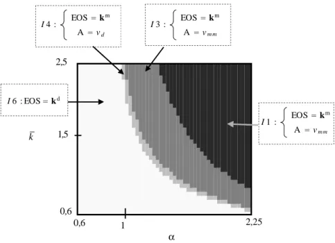
Assume that M = 5,G = 0.1, kG = 1.5, Λ = a−c = 6 and G = 0,1. For simplicity, using a low cost of greenfield entry then implies that the probability of greenfield entry Ph is set to unity. In fig A.2, we first illustrate the implied Equilibrium Ownership Structure (EOS) over the α k¯ -space. This figure illustrates proposition 1 as α must be sufficiently high for an acquisition to occur (i.e. α >1). In figure A.3, we calculate the implied change in stockmarket value for the acquirer as compared to a situation where no acquisition takes place. The change in stockmarket value is then measured the difference between net-profits of the acquiring MNE, ΠA(km), and its pre-merger announcement value, i.e. ΠA(km)−E ΠG(kd) = ΠA(km)−Pd πG(kd)−G . This figure illustrates the statement in corollary 1 that the stockmarket value of the acquirer may decrease (at high values ofα) or increase (at low values ofα).
I 3 : EOSk m A vm m I 1 : EOSk m A vm m I 6 : EOSkd 6 0, 2,25 α 1 6 0, 5 2, k 1,5 I 4 : EOSk m A vd
Figure A.2: Equilibrium Ownership Structure (EOS).
0,6 0,6 -0,6 -0,5 -0,4 -0,3 -0,2 -0,1 0 0,1 0,2 0,3 -0,6 -0,5 -0,4 -0,3 -0,2-0,2 -0,1 0 0,1 0,2 0,3 2,25 2,5 0,6 0,6 -0,6 0 0,3 α k $Akm "E $Gkd t
References
[1] Bjorvatn, K., 2001, “On the Profitability of Cross-Border Mergers, Mimeo, LOS, Bergen.
[2] Business Week, October 2, 2000, November 20, 2000, April 23, 2001.
[3] Caves, R.E., 1996. Multinational Enterprise and Economic Analysis. 2nd edition, (Cambridge University Press, Cambridge and New York).
[4] Das, S P. and Sengupta, S.,2001, ”Assymetric information, Bargaining, and Inter-national Mergers”, Journal of Economics and Management Strategy, Vol 10, No 4, 565-590.
[5] Dixit, A. and C. Shapiro, 1986, ”Entry Dynamics and Mixed Strategies.” In The Economics of Strategic Planning: Essays in Honor of Joel Dean, edited by L. G. Thomas. Lexington Books.
[6] Dunning, J., Trade, 1977, Location of Economic Activity and the MNE: A Search for and Eclectic Approach, in: Ohlin, B. Hesselborn, P.-O. and P.M. Wijkman, eds, The International Allocation of Economic Activity, (London: McMillan) 395-418. [7] The Economist, September 21, 2000.
[8] Farrell, J and Shapiro, C, “Asset Ownership and Market Structure in Oligopoly,”
RAND Journal of Economics, Summer 1990b, Vol. 21, 275-292.
[9] Fridolfsson, S.-O. and J. Stennek, 1999, ”Why Mergers Reduce Profits, and Raise Share Prices,” Working Paper No. 511, (Stockholm: The Research Institute of In-dustrial Economics).
[10] Görg, H., 2000, “Analyzing Foreign Market Entry: The Choice between Greenfield Investment and Acquisition,” Journal of Economic Studies.
[11] Head K, and J. Reis, 1997, ”International Mergers and Welfare under Decentralized Competition Policy”, Canadian Journal of Economics v30, n4: 1104-23.
[12] Horn, H. and L. Persson, 2001, “The Equilibrium Ownership of an International Oligopoly,”Journal of International Economics, Vol. 53, No. 2.
[13] Kamien, M. I. and Zang, I., 1990, “The Limits of Monopolization Through Acqui-sition,” Quarterly Journal of Economics, 2, 465-99.
[14] Markusen, J. R., 1995, ”The Boundaries of Multinational Enterprises and the The-ory of International Trade,” Journal of Economic Perspectives 9, 169-189.
[15] Nti, K. O., 2000, ”Potential Competition and Coordination in a Market Entry Game,” Journal of Economics, Vol. 71, N0.2. 149-165.
[16] Scherer, F. M., and Ross, D., 1990, ”Industrial Market Structure and Economic Performance,” Houghton Mifflin Company.
[17] UNCTAD, World Investment Report 2000, (United Nations Conference on Trade and Development, Geneva).
[18] Vives, X. 1988, ”Sequential Entry, Industry Structure and Welfare, ” European