Antitrust Policy and Environmental Protection
Shigeru Matsumoto Hajime Sugeta
Kansai University Kansai University
Abstract
We examine the effects of antitrust policy (the prohibition of a input price discrimination) when an emission tax is used for environmental protection. We show that antitrust policy reduces pollution emission and improves social welfare. Therefore, antitrust policy contributes to environmental protection.
An earlier version of this paper is presented at the SEEPS 2005 conference, Tokyo and the ISS industrial Organization Workshop at Tokyo University. We would like to thank Yasunori Fujita, Norimichi Matsueda, Toshihiro Matsumura, Dan Sasaki, and other participants for the useful comments. We also thank the associate editor and anonymous referee for valuable comments.
1
Introduction
The welfare effect of third-degree price discrimination has been intensively studied in the
last century.1 However, most studies have examined the relationship between total output
and social welfare. We employ the standard model of input price discrimination proposed
by Katz (1997) and DeGraba (1990) and examine the effects of a typical antitrust
pol-icy (the Robinson-Patman Act) on environmental protection.2 The downstream market
comprises Cournot duopoly firms that produce the final product for consumers. They use two intermediate inputs. One is a dirty input that is supplied in a competitive
mar-ket; its use causes environmental pollution. The other is a clean input that is supplied
by the monopolist; its use does not cause any environmental pollution. The two
down-stream firms have different production technologies and use the dirty input in different quantities. We refer to the firm that uses a lesser amount of the dirty input as an envi-ronmentally friendly firm. We refer to the other firm as an environmentally unfriendly
firm. The difference in thesefirms’ production technologies provides the monopolist with an incentive to price discriminate against them.
We assume that the pollution damage is serious, and the environmental protection
agency (EPA) levies an emission tax on pollution emission. We then examine the effects
of a specific antitrust policy (the prohibition of an input price discrimination) in two cases.3 In the first case, EPA has to utilize the same tax rate regardless of the pricing regime. In the second case, EPA differentiates between the tax rates of two pricing
regimes so as to maximize social welfare.
1See Schmalensee(1981), Varian(1985), and Schwartz(1990)for the reference.
2Yoshida (2000) and Valletti (2003) generalized the analysis of input price discrimination. More recently, Adachi (2002,2005) examines the welfare consequence of third-degree price discrimination in the presence of consumption externalities. Galera and Zaratiegui(2005) generalizes the analysis to an oligopoly framework.
3In this paper, the application of antitrust policy implies the prohibition of an input price discrimina-tion by a monopolist. The result presented in this paper may not be valid for different kinds of antitrust policies.
2
The Model
Two Cournot downstream firms produce a homogeneous final product and engage in quantity competition. Letqi and qj denote the quantities of the final product produced byfirmiandfirmj, respectively. The aggregate supply is indicated byQ≡Pqi ≡qi+qj. The downstreamfirms produce their products using two types of inputs: a clean input and a dirty input. The clean input is supplied by the upstream monopolist M, while
the dirty input is supplied in a competitive market. The monopolist produces the clean
input at a constant marginal cost cM.
The downstream firms have Leontief-type technologies. The firm i requires one unit of the clean input andβi units of the dirty input to produce one unit of thefinal product.
Let ei denote the amount of pollution emission by firm i. One unit of the dirty input leads to one unit of pollution emission, i.e., ei = βiqi. We assume βi < βj. Thus, firm i uses a smaller amount of the dirty input than firm j to produce one unit of the final product. We refer to firm i andfirm j as environmentally friendly and environmentally unfriendly firms, respectively. The aggregate emission is given byE ≡Pei.
The consumers’ utility level,U, is assumed to be additively separable from the
disutil-ity arising from the environmental damage,D(E)≡ϕE. Thus,U =u(Q) +m−D(E), whereu(Q)≡aQ−12bQ2 andmis the numeraire consumption. Letpdenote the price of
thefinal product. From utility maximization by the consumers, it follows thatp=u0(Q). Thus, the downstream firms face the linear inverse demand function, p(Q)≡a−bQ.
EPA imposes an emission tax rate ofτ. We normalize the price of the dirty input to1.
Then, the profit function of the downstream firmiis given by πi ≡(p(Q)−ri−βi)qi−
τei, whereri is the price of the intermediate input. When price discrimination is
prohib-ited by the antitrust law, ri =rj =r. The profit function of the monopolist is given by πM ≡P(ri−cM)qi.
In the subsequent analysis, we consider the two-stage game. In Stage 1, the
order to find the subgame perfect equilibrium of this stage game, the usual backward induction is employed. Thus, we begin with solving the second-stage problem.
2.1
Downstream Market
The second-stage game is characterized by Cournot duopoly with eachfirm incurring the marginal cost,ci ≡ri+βi(1+τ). We obtain the following equilibrium outputs under price discrimination:4 qd
i = 31b(a−2ri+rj−(2βi−βj)(1 +τ))andQd= 32b
¡
a−r+β(1 +τ)¢, where r ≡ 12(ri+rj) is the average input price and β ≡ 12¡βi+βj
¢
is the average
pollution intensity of the twofirms. If price discrimination is prohibited, i.e.,ri =rj =r, then the equilibrium outputs become qu
i =
1
3b(a −r − (2βi − βj) (1 +τ)) and Qu =
2
3b(a−r+β(1+τ)). Furthermore, the second-stage Cournot-Nash equilibrium downstream
profit and total emission level can be expressed as πx
i = b(qix)
2
and Ex
≡ Pβiqx i,
respectively, for the pricing regimex=d, u.
2.2
Upstream Market
Under price discrimination, the monopolist maximizes its profit πd
M ≡
P
(ri−cM)qd i
with respect tori andrj. This yields the discriminatory prices given byri = 12(a+cM−
βi(1 +τ)). Since ri−rj = 12(βj −βi)(1 +τ) > 0, the environmentally friendly firm is
charged a higher input price than the environmentally unfriendlyfirm. Firmi’s marginal cost becomes cd
i =
1
2(a+cM +βi(1 +τ)).
The uniform pricing regime yields the profit function of the monopolist, given by πuM ≡
P
(r−cM)qui = (r−cM)Qu. After substituting the aggregate input demand
and then maximizing πuM through the choice of r, we obtain the optimal uniform price,
r= 12(a+cM −β(1 +τ)), which is the average of the optimal discriminatory prices, i.e.,
r=r. Firm j’s marginal cost becomes cu i =
1
2(a+cM +
¡
2βi−β¢(1 +τ)).
4The superscript d denotes the discriminatory pricing regime, while the superscript u denotes the uniform pricing regime.
The antitrust policy changes the pricing regime from price discrimination to uniform
pricing. It doubles the cost difference between the two downstreamfirms, sincecu
j−cui =
(βj − βi)(1 + τ) = 2(cdj − cdi) > 0. Therefore, the antitrust policy strengthens the
competitiveness of the environmentally friendly firm.
For an exogenously given emission tax, the equilibrium outcomes are summarized in
the left column of Table 1. It follows thatqd
i −qjd=
1
2b(1 +τ)
¡
βj−βi¢ >0. Thus, the discriminatory pricing does not reverse the marginal cost ranking.
We can show that ∂(ri −rj)/∂τ = 12(βj −βi) > 0. The degree of the input price
discrimination rises when the emission tax is increased. We also know that the tax
increase relatively favors the environmentally friendlyfirm,∂(cd
j−cdi)/∂τ = 1 2(βj−βi)>0. Hence, we obtain ∂(qd i −qjd)/∂τ = 1 2b ¡
βj −βi¢>0. The tax increase widens the output difference between the two downstreamfirms.
The output difference under uniform pricing is qu
i −quj = 1b (1 +τ)
¡
βj−βi¢ > 0; thus, ∂(qui −qju)/∂τ = 2 ·∂(qid−qjd)/∂τ > 0. This implies that the effect of the tax
increase on the output difference is stronger under price discrimination.
Finally, we examine the effectiveness of the emission tax under both pricing regimes.
By differentiating the total emission with respect to τ, we can compare the effectiveness
of the emission taxation between the two pricing regimes as follows:
0>− 1 3bK = ∂Ed ∂τ > ∂Eu ∂τ =− 1 3b(2K −β 2 ), where we define K ≡ β2i −βiβj +β 2 j > 0 and employ 2K −β 2 > K ⇔ K −β2 = 3¡βj−βi ¢2 /4>0.
Lemma 1 Antitrust policy increases the effectiveness of the emission taxation.
2.3
Optimal Emission Tax Rates
We now derive the optimal tax rates under both pricing regimes. The social welfare is P
the consumer’s surplus net of the environmental damage, the next two terms are the
upstream and downstream profits, and the last term is the tax revenue. Substituting the above expressions into u(Q), πM, πi and D(E), we write the social welfare under the
pricing regime x=d, uas Wx =AQx− 1 2b(Q x)2 −Xβiqxi −ϕE x,
where A ≡ a−cM > 0. Differentiating W with respect to τ, we obtain the first-order condition for the optimal emission tax rate:
dWx dτ = (A−bQ x)dQx dτ −(1 +ϕ) dEx dτ = 0.
Substituting the comparative statics results under each regime, we obtain the optimal
total outputs for the pricing regimex=d,u. We denote them asQx∗ in the right column of Table 1, together with the other optimal outcomes. Solving Qx∗ =Qx forτ yields the
optimal rate of emission tax for both regimes:
τd = 3K(1 +ϕ)−2Aβ β2 −1, τ u = 3(2K −β 2 ) (1 +ϕ)−2Aβ β2 −1.
When these optimal tax rates are utilized, both downstream firms produce positive out-put. The difference between these two optimal tax rates isτu
−τd = (K
−β2) (1 +ϕ)/(3β2)>
0, since K−β2 >0.
Lemma 2 The optimal emission tax rate under price discrimination is lower than that under uniform pricing.
We assume that the pollution damage is serious. Therefore, the parameters are
re-stricted as follows:
This assumption implies that 1 +τu and 1 +τd are both positive. Since τu > τd,
1 +τd >0 is sufficient. However, we require the condition for 1 +τu >0 to prove that
∆E∗ is negative.
3
Welfare E
ff
ect of the Antitrust Policy
3.1
First Case: EPA cannot set the tax rate.
EPA has to utilize the same tax rate regardless of the pricing regime. Using the
equilib-rium outcomes presented in the left column of Table 1, we can examine the welfare effect
of the antitrust policy.
First, we find∆Q ≡ Qu −Qd = 0 and∆E ≡Eu −Ed = −1 3b(1 +τ) (K −β 2 ) <0. The total output is unaffected by the regime change while total emission is reduced.
However, the environmental condition is improved by the antitrust policy. If consumer
welfare is given by the difference between consumer surplus and pollution damage, then
antitrust policy improves it.
We now evaluate the welfare effect of the antitrust policy as follows: ∆W =−Pβi∆qi
−ϕ∆E. When price discrimination is permitted, the monopolist charges the environmen-tally friendly firm a higher input price than it does the environmentally unfriendly firm. Antitrust policy shifts the production from the environmentally unfriendly firm to the environmentally friendlyfirm, while maintaining the aggregate output at the same level. This resolves the production inefficiency, which is captured by the term, Pβi∆qi < 0. Furthermore, the antitrust policy reduces the total pollution emission and mitigates
the pollution problem. Therefore, it also resolves the environmental inefficiency. From
E = Pβiqi, two welfare gains (production and environmental efficiencies) obtained by
the antitrust policy amount to ∆W = 41b (1 +ϕ) (1 +τ)¡βj −βi¢2 >0.
Proposition 1 When an emission tax rate is exogenously determined, social welfare is improved by antitrust policy.
3.2
Second Case: EPA optimizes the tax rate.
EPA now sets the emission tax rate. By substituting the optimal emission tax rates into
the corresponding conditions, we obtain equilibrium outcomes as given in Table 1.
The change in total output is ∆Q∗ = −(1 +ϕ) (K −β2)/(bβ) < 0. Therefore, the
total output is reduced by the antitrust policy.
The change in total emission is
∆E∗ = 1
3bβ2(K−β
2
)³2Aβ−3(3K −β2) (1 +ϕ)´
Assumption 1 requires2Aβ <3K(1 +ϕ). From3K−β2 > K, it follows that∆E∗ <0.
The change in social welfare is
∆W∗ = 1
6bβ2(1 +ϕ) (K−β
2
)³3(3K−β2) (1 +ϕ)−4Aβ´
Assumption 1 requires4Aβ to be under6K(1 +ϕ). From3K−β2 >2K, it follows that
∆W∗ >0. This implies that antitrust policy improves social welfare.
Proposition 2 When an emission tax rate is optimally chosen, social welfare is in-creased by antitrust policy.
4
Conclusion
This note has examined the effect of antitrust policy when an emission tax is used for
environmental protection. We consider two cases. In the first case, it is assumed that the same emission tax rate is applied regardless of the pricing regime. In the second
case, it is assumed that the emission tax rate is optimized depending on the pricing
regime. In both cases, we show that antitrust policy (the prohibition of an input price
enhances the effectiveness of the pollution taxation. The joint use of pollution taxation
and antitrust policy is favorable for environmental protection.
References
[1] Adachi, T., (2005). A note on third-degree price discrimination with interdependent
demands. Journal of Industrial Economics 50, 171-178.
[2] Adachi, T., (2005). Third-degree price discrimination, consumption externalities and
social welfare. Economica 22, 171-178.
[3] DeGraba, P., (1990). Input market price discrimination and the choice of technology.
American Economic Review 80, 1246-1253.
[4] Galera, F. and Zaratiegui, J., (2006). Welfare and output in third-degree price
dis-crimination: A note.International Journal of Industrial Organization 24, 605-611.
[5] Katz, M., (1987). The welfare effects of third-degree price discrimination in
inter-mediate good markets. American Economic Review 77, 154-167.
[6] Schmalensee, R., (1981). Output and welfare implications of monopolistic
third-degree price discrimination. American Economic Review 71, 242-247.
[7] Schwartz, M., (1990). Third-degree price discrimination and output: Generalizing a
welfare result.American Economic Review 80, 1259-1262.
[8] Valletti, T., (2003). Input price discrimination with downstream Cournot
competi-tors. International Journal of Industrial Organization 21, 969-988.
[9] Varian, H., (1985). Price discrimination and social welfare. American Economic
Review 75, 870-875.
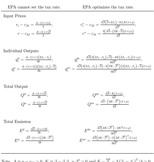
Table 1. Equilibrium Outcomes
Case 1 Case 2
EPA cannot set the tax rate. EPA optimizes the tax rate.
Input Prices ri −cM = A−(1+τ)βi 2 ; r∗i −cM = Aβ(β+2βi)−3βiK(1+ϕ) 2β2 ; r−cM = A−(1+2 τ)β r∗ −cM = 3(Aβ−(2K−β)(1+ϕ)) 2β Individual Outputs qd i = A−(1+τ)(2βi−βj) 6b ; q d∗ i = Aβ(2(2βi−βj)+β)−3K(2βi−βj)(1+ϕ) 6bβ2 ; qu i = A−(1+τ)(2(2βi−βj)−β) 6b q u∗ i = Aβ(4(2βi−βj)−β)−3³2K−β2´(2(2βi−βj)−β)(1+ϕ) 6bβ2 Total Output Qd= A−(1+τ)β 3b ; Q d∗ = Aβ−K(1+ϕ) bβ ; Qu = A−(1+τ)β 3b Q u∗ = Aβ− ³ 2K−β2´(1+ϕ) bβ Total Emission Ed= Aβ−(1+τ)K 3b ; E d∗ = Aβ ³ 2K+β2´−3K2(1+ϕ) 3bβ2 ; Eu = Aβ−(1+τ) ³ 2K−β2´ 3b E u∗ = Aβ ³ 4K−β2´−3³2K−β2´2(1+ϕ) 3bβ2 Note. A≡a−cM >0, K ≡β−βiβj+β 2 j >0 andK−β 2 = 3¡βi−βj ¢2 /4>0.