A new algorithm for topology optimization using a level-set method

(1)

S. Amstutz, H. Andrä

A new algorithm for topology

(2)

ISSN 1434-9973

Bericht 78 (2005)

Herausgebers ist es nicht gestattet, das Buch oder Teile daraus in irgendeiner

Form durch Fotokopie, Mikroﬁ lm oder andere Verfahren zu reproduzieren

oder in eine für Maschinen, insbesondere Daten ver ar be i tungsanlagen,

ver-wendbare Sprache zu übertragen. Dasselbe gilt für das Recht der öffentlichen

Wiedergabe.

Warennamen werden ohne Gewährleistung der freien Verwendbarkeit benutzt.

Die Veröffentlichungen in der Berichtsreihe des Fraunhofer ITWM können

bezogen werden über:

Fraunhofer-Institut für Techno- und

Wirtschaftsmathematik ITWM

Gottlieb-Daimler-Straße, Geb. 49

67663 Kaiserslautern

Germany

(3)

Vorwort

Das Tätigkeitsfeld des Fraunhofer Instituts für Techno- und Wirt schafts ma the ma tik

ITWM um fasst an wen dungs na he Grund la gen for schung, angewandte For schung

so wie Be ra tung und kun den spe zi ﬁ sche Lö sun gen auf allen Gebieten, die für

no- und Wirt schafts ma the ma tik be deut sam sind.

In der Reihe »Berichte des Fraunhofer ITWM« soll die Arbeit des Instituts kon ti

nu ier lich ei ner interessierten Öf fent lich keit in Industrie, Wirtschaft und Wis sen

-schaft vor ge stellt werden. Durch die enge Verzahnung mit dem Fachbereich

the ma tik der Uni ver si tät Kaiserslautern sowie durch zahlreiche Kooperationen mit

in ter na ti o na len Institutionen und Hochschulen in den Bereichen Ausbildung und

For schung ist ein gro ßes Potenzial für Forschungsberichte vorhanden. In die

richt rei he sollen so wohl hervorragende Di plom und Projektarbeiten und Dis ser

-ta ti o nen als auch For schungs be rich te der Institutsmi-tarbeiter und In s ti tuts gäs te zu

ak tu el len Fragen der Techno- und Wirtschaftsmathematik auf ge nom men werden.

Darüberhinaus bietet die Reihe ein Forum für die Berichterstattung über die

rei chen Ko o pe ra ti ons pro jek te des Instituts mit Partnern aus Industrie und

schaft.

Berichterstattung heißt hier Dokumentation darüber, wie aktuelle Er geb nis se aus

mathematischer For schungs- und Entwicklungsarbeit in industrielle An wen dun gen

und Softwareprodukte transferiert wer den, und wie umgekehrt Probleme der

xis neue interessante mathematische Fragestellungen ge ne rie ren.

Prof. Dr. Dieter Prätzel-Wolters

Institutsleiter

(4)

(5)

A new algorithm for topology optimization

using a level-set method

Samuel Amstutz

a

, Heiko Andr¨a

a

Fraunhofer Institut f¨

ur Techno- und Wirtschaftsmathematik,

Gottlieb-Daimler-Str. 49, D-67663 Kaiserslautern, Germany.

Abstract

The level-set method has been recently introduced in the field of shape

optimiza-tion, enabling a smooth representation of the boundaries on a fixed mesh and

there-fore leading to fast numerical algorithms. However, most of these algorithms use a

Hamilton-Jacobi equation to connect the evolution of the level-set function with the

deformation of the contours, and consequently they cannot create any new holes in

the domain (at least in 2D). In this work, we propose an evolution equation for the

level-set function based on a generalization of the concept of topological gradient.

This results in a new algorithm allowing for all kinds of topology changes.

Key words:

shape optimization, topology optimization, topological sensitivity,

level-set.

1991 MSC:

65K05, 65K10, 74B05, 74F10, 74P05, 74P15

1

Introduction

Many methods have been worked out for the automatic optimization of

elas-tic structures. The oldest and most popular one, the so-called classical shape

optimization method [20,26], is based on the computation of the sensitivity of

the criterion of interest with respect to a smooth variation of the boundary. Its

main drawback is that it does not allow any topology changes. To overcome

this limitation, relaxed formulations using

e.g.

the homogenization theory have

been introduced [1,2,6,9,10,17]. However, these methods are mainly restricted

to linear elasticity and particular objective functions. Despite their high

com-putational cost, stochastic algorithms (like genetic algorithms, see

e.g.

[18])

Email addresses:

[email protected]

(Samuel Amstutz),

[email protected]

(Heiko Andr¨a).

(6)

can be used to deal with more general situations, or when a sensitivity

com-putation is complicated because of practical reasons (for instance the adjoint

state may not be computable by available softwares).

The level-set method, which has several advantages, was investigated by Osher

and Sethian [22] for numerically tracking fronts and free boundaries, and

re-cently introduced in the field of shape optimization [4,5,11,21,24,27]. First, its

main feature is to enable an accurate description of the boundaries on a fixed

mesh. Therefore it leads to fast numerical algorithms. Second, its range of

application is very wide, since the front velocity can be derived from the

clas-sical shape sensitivity. Finally, it can handle some kinds of topology changes,

namely the merging or cancellation of holes. However, the usual choice of a

Hamilton-Jacobi equation to control the evolution of the level-set function

im-plies that this latter obeys a maximum principle. The immediate consequence

of this property is that the nucleation of holes inside the domain is

prohib-ited. Holes can only appear by pinching two boundaries, which is possible in

3D but not in 2D. It follows that in this case the obtained design is strongly

dependent on the initial guess which decides of the maximum number of holes

allowed.

Besides, the notion of topological gradient [15,19,23,25] has been devised to

measure the sensitivity of a criterion with respect to the size of a small hole

created around a given point of the domain. This concept gave rise to another

class of shape optimization algorithms. Generally, they proceed by iterative

removal of matter where the topological gradient is less than a certain

thres-hold, which plays the role of a step size and which is determined more or less

automatically. Their main drawback is their inability to add matter in some

places where it has been removed “by mistake” at previous iterations.

In this paper, we propose an evolution equation for the level-set function based

on a generalization of the concept of topological gradient. This results in a

new algorithm allowing for all kinds of topology changes. Its convergence to

a (local) minimum is illustrated by several numerical experiments performed

in the contexts of structural mechanics and porous media flows. In order to

decrease the number of these local minima, which may exist even when no

topological constraint is imposed, a filtering technique is used, acting in a

similar way as a regularization. The basic difference between our algorithm

and others, which have been developed in the same direction [3,12,28] is that

we have completely abandoned the Hamilton-Jacobi equation, avoiding in this

way all arbitrary parameters involved in the construction of a correction.

(7)

2

Presentation of a model problem

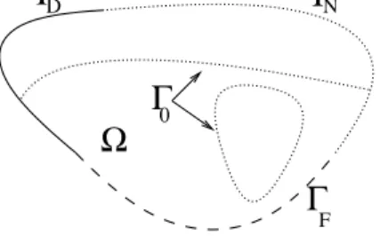
Let

D

be a smooth domain of

R

d

(d

= 2 or 3) and Ω be a smooth subdomain

of

D

occupied by a linear isotropic elastic material. The latter stands for the

design domain,

i.e.

the domain we want to optimize, whereas the former is

a fixed set meant to define the maximum bulk of the structure as well as to

serve as a computational box. The boundary

∂D

of

D

is made of the three

disjoint parts

∂D

= Γ

D

∪

Γ

F

∪

Γ

N

,

with Γ

D

of nonzero Lebesgue measure. We assume that the boundary of Ω

satisfies

∂Ω = (Γ

D

∩

∂Ω)

∪

Γ

F

∪

(Γ

N

∩

∂Ω)

∪

Γ

0

,

where Γ

0

=

∂

Ω

∩

D

(see Fig. 1). For a given load

ϕ

∈

(H

−1/2

(Γ

F

))

d

, the linear

elasticity equations for the displacement

u

Ω

read as follows:











−

div (Ae(u

Ω

)) = 0 in Ω,

u

Ω

= 0 on Γ

D

∩

∂Ω,

(Ae(u

Ω

))n

=

ϕ

on Γ

F

,

(Ae(u

Ω

))n

= 0 on (Γ

N

∩

∂Ω)

∪

Γ

0

.

(1)

In this system,

A

denotes the Hooke’s tensor of the material and

e(u

Ω

) denotes

the linearized strain tensor. Note that the part Γ

F

of the border where the

load is applied is prescribed.

Γ

D

Γ

N

Γ

₀

Ω

F

Γ

Figure 1. The working domain

D

.

To fix ideas, we consider a criterion

j(Ω) made of the compliance

comple-mented with a term accounting for the weight of the structure,

i.e.

(8)

where the functional

J

is defined on (H

1

(Ω))

d

by

J(u) =

Z

ΓF

ϕ.uds

(3)

and

|

Ω

|

is the Lebesgue measure of Ω. The constant

` >

0 is given and can be

interpreted as a Lagrange multiplier. Due to the Green’s formula, the

compli-ance can also be computed by

J(u

Ω

) =

Z

Ω

Ae(u

Ω

) :

e(u

Ω

)dx.

(4)

However, we will prefer the formulation (3) which turns out to be more

con-venient from the numerical point of view. We are interested in the topological

shape optimization problem

inf

Ω∈Uad

j(Ω),

with

U

ad

=

{

Ω

⊂

D,

Γ

F

⊂

∂Ω,

meas (Γ

D

∩

∂Ω)

6

= 0

}

.

By (4) and the Korn’s inequality, the above infimum exists in

R

+

, but it

is generally not reached in this set of admissible domains. Nevertheless, the

algorithm we will present only requires the existence of a local minimum.

To avoid remeshing, the elasticity problem (1) is approximated by the

follow-ing, formulated in the fixed domain

D:











−

div ( ˜

αAe(u

Ω

)) = 0 in

D,

u

Ω

= 0 on Γ

D

,

(Ae(u

Ω

))n

=

ϕ

on Γ

F

,

(Ae(u

Ω

))n

= 0 on Γ

N

,

(5)

with

˜

α

=











1 in Ω,

ε

in

D

\

Ω.

(6)

The constant

ε

must be chosen small enough to mimic Problem (1) with a

suitable accuracy. In the computations presented in Sections 4 and 5, the

value

ε

= 10

−3

has been used.

(9)

3

Description of the algorithm

3.1

Topological sensitivity

At a point

x

∈

Ω, the topological gradient

g(x) is a number that measures the

sensitivity of the criterion

j(Ω) with respect to the creation of a small hole

around

x. More precisely, it is defined by the topological asymptotic expansion:

j(Ω

\

B(x, ρ))

−

j(Ω) =

f

(ρ)g(x) +

o(f

(ρ)),

(7)

where

B(x, ρ) is the ball of center

x

and radius

ρ

and

f

(ρ) is a smooth positive

function going to zero with

ρ. In this work, only circular or spherical holes are

considered although such an expansion can be obtained for arbitrary shaped

holes and also for cracks.

Actually, in our algorithm, it is interesting to consider not the creation of a

real hole but the insertion of the soft material we have introduced to simulate

void. As expected, the comparison of the corresponding asymptotic expansions

shows that the sensitivities with respect to both kinds of perturbation tend

to be identical when the density

ε

tends to zero. However, the advantage of

this approach is that it allows for the opposite operation,

i.e.

to strengthen

the weak phase.

In [8], the asymptotic expansion (7) has been generalized to the case where

the density ˜

α

inside the ball

B(x, ρ) is shifted from its initial value

α

0

into the

new value

α

1

. Combining this general result with the elastic moment tensor

calculated in [7], we obtain in linear elasticity 2D plane strain the expression:











f

(ρ) =

|

B(x, ρ)

|

,

g(x) =

r

−

1

κr

+ 1

κ

+ 1

2

"

2σ(u

Ω

) :

e(v

Ω

) +

(r

−

1)(κ

−

2)

κ

+ 2r

−

1

trσ(u

Ω

)tre(v

Ω

)

#

+

`δ,

with

r

=

α

1

α

0

,

κ

=

λ

+ 3µ

λ

+

µ

.

The constants

λ

and

µ

are the Lam´e coefficients and the stress tensor

σ(u

Ω

) is

computed with the local density at the point

x. In plane stress,

λ

∗

= 2µλ/(λ

+

2µ) must be substituted for

λ. The displacement field

v

Ω

is the adjoint state

and the binary variable

δ

is introduced for convenience to indicate the sense

of the variation of surface of Ω:

δ

=











−

1 if

|

Ω

|

is decreased (creation of a hole),

(10)

For the cost functional (3), the problem is well-known to be self-adjoint,

i.e.

v

Ω

=

−

u

Ω

.

In our case,

α

0

and

α

1

can only take the values 1 and

ε. When

α

0

= 1, the

only perturbation possible is the creation of a hole, which means that

α

1

=

ε,

r

=

ε

and

δ

=

−

1. The associated gradient is

g

−

(x) =

ε

−

1

κε

+ 1

κ

+ 1

2

"

2σ(u

Ω

) :

e(v

Ω

) +

(ε

−

1)(κ

−

2)

κ

+ 2ε

−

1

trσ(u

Ω

)tre(v

Ω

)

#

−

`.

When

α

0

=

ε, we have to consider a reinforcement,

i.e.

α

1

= 1,

r

= 1/ε

and

δ

= +1. The associated gradient is

g

+

(x) =

1

−

ε

κ

+

ε

κ

+ 1

2

"

2σ(u

Ω

) :

e(v

Ω

) +

(1

−

ε)(κ

−

2)

κε

+ 2

−

ε

trσ(u

Ω

)tre(v

Ω

)

#

+

`.

As said before,

g

−

as well as

g

+

can be accurately computed by taking

ε

= 0

in the above expressions. We define the quantity

˜

g(x) =











−

g

−

(x) if

x

∈

Ω,

g

+

(x) if

x

∈

D

\

Ω

(9)

that measures the sensitivity of the criterion

j(Ω) with respect to an oriented

shift of the density. It follows that a necessary local minimality condition for

the approximated problem (5) is











˜

g(x)

≤

0 in Ω,

˜

g(x)

≥

0 in

D

\

Ω,

(10)

and that a sufficient local minimality condition for this class of domain

per-turbations is











˜

g(x)

<

0 in Ω,

˜

g(x)

>

0 in

D

\

Ω.

(11)

3.2

Representation by a level-set function

As it is common in level-set methods, we introduce a fictitious time

t

and

we consider a family of domains (Ω(t))

t≥0

. This family is represented by a

(11)

level-set function

ψ

:

R

×

D

→

R

such that











ψ(t, x)

<

0

⇐⇒

x

∈

Ω(t),

ψ(t, x)

>

0

⇐⇒

x

∈

D

\

Ω(t),

ψ(t, x) = 0

⇐⇒

x

∈

Γ

0

(t).

(12)

For our topological shape optimization problem, we choose

ψ

as a design

vari-able. We denote by ˜

g(t, x) the generalized topological gradient associated to

the domain Ω(t) and computed at the point

x. Instead of governing the

evo-lution in time of the level-set function by a Hamilton-Jacobi equation

propa-gating the interface Γ

0

(t), we propose the equations

ψ(0, .)

∈ S

,

(13)

∂ψ

∂t

=

P

ψ⊥

(˜

g)

∀

t

≥

0,

(14)

where

P

ψ⊥

is the orthogonal projector onto the orthogonal complement of

ψ,

i.e.

P

ψ⊥

(˜

g) = ˜

g

−

(˜

g, ψ)

k

ψ

k

2

ψ.

In the above relations, the inner product (., .), the norm

k

.

k

as well as the unit

sphere

S

refer to the Hilbert space

L

2

(D). The solution of (13), (14) satisfies

the following outstanding properties.

(1) It comes straightforwardly (

i.e.

by multiplying both sides of Equation

(14) in the sense of the inner product by

ψ) that

ψ(t, .)

∈ S

∀

t

≥

0.

(2) If

ψ

tends to a stationary point and if the topological gradient ˜

g

at that

point is nonzero, then it is a local optimum of the topological shape

opti-mization problem. Indeed, the relation

P

ψ⊥

(˜

g) = 0 implies the existence

of a real number

s

such that ˜

g

=

sψ. If

s >

0, then the conditions (11)

are fulfilled and we are in the presence of a local minimum. If

s <

0,

then a local maximum has been reached. However this latter situation is

highly unlikely since the right hand side of the transport equation has

been chosen in order decrease the criterion.

3.3

Numerical algorithm

Let

U

h

be a finite dimensional subspace of

L

2

(D). It is endowed with the

(12)

is a level-set function

ψ

living in the unit ball

S

h

of

U

h

. The elasticity problem

(5) is solved by means of a finite element method such that the resulting

approximation ˜

g

h

of the topological gradient is obtained (or projected) in

U

h

. In the sequel, for notational simplicity, all indexes

h

referring to a finite

element approximation will be omitted.

The time is discretized by a sequence (t

i

)

i∈N

such that the variation of the

topological gradient can be neglected in the interval [t

i

, t

i+1

]. Like in [5], the

time step is automatically reduced if the criterion

j(Ω) is increasing. In this

way, the evolution equation (14) can be solved analytically in the interval

[t

i

, t

i+1

] (Euler’s method on the sphere): there exists an angle

ξ

i

∈

[0, θ

i

] such

that

ψ

i+1

= cos

ξ

i

.ψ

i

+ sin

ξ

i

.

P

ψ⊥ i

(˜

g

i

)

k

P

ψ⊥ i

(˜

g

i

)

k

.

(15)

The notations

ψ

i

(x) =

ψ(t

i

, x) and ˜

g

i

(x) = ˜

g(t

i

, x) are used and

θ

i

is the

non-oriented angle between the vectors

ψ

i

and ˜

g

i

,

i.e.

θ

i

= arccos

(ψ

i

,

g

˜

i

)

k

g

˜

i

k

.

For numerical purposes, we have interest to make the change of variable

ξ

i

=

κ

i

θ

i

,

κ

i

∈

[0,

1].

By using trigonometric formulas we arrive easily at the relation

ψ

i+1

=

1

sin

θ

i

"

sin((1

−

κ

i

)θ

i

).ψ

i

+ sin(κ

i

θ

i

).

˜

g

i

k

˜

g

i

k

#

.

(16)

Therefore we propose the following algorithm.

(1) Choose an initial level-set function

ψ

0

∈ S

and an initial step

κ

0

.

(2) Iterate until target is reached:

•

construct the domain Ω

i

by (12),

•

solve the elasticity problem (5) and compute the topological gradient

˜

g

i

by (9),

•

update the level-set function by (16) with a step

κ

i

chosen according

to the previous iteration and possibly decreased until the criterion

de-creases.

In all computations, we have used a triangular mesh so that arbitrary

geome-tries can be handled. Finite elements of order 1 are used to solve the elasticity

equations as well as to represent the level-set function. In the cells that are

(13)

crossed by the curve of equation

ψ

= 0, the density ˜

α

in (5) as well as the

topological gradient ˜

g

are computed by linear interpolation.

In order to impose some smoothness on the domain and, in the same time, to

decrease the number of local minima, a filtering technique based on a reduction

of the number of design variables may be useful (see

e.g.

[14]). In our context,

this is achieved by discretizing the level-set function on a mesh which is coarser

than the one used for solving the elasticity equations and by projecting the

topological gradient onto the finite elements space associated to this coarse

mesh. For the sake of coherence, an orthogonal projection with respect to the

inner product of

L

2

(D) is performed.

The following section is devoted to the validation of the algorithm on classical

examples. A more complicated problem is addressed in Section 5.

4

Numerical examples in linear elasticity

4.1

Cantilever

The first example is the cantilever problem that has been treated

e.g.

in [5].

The computational box

D

is a rectangle of size 2

×

1 with an homogeneous

Dirichlet condition on the left side and a vertical pointwise unitary load applied

at the middle of the right side (see Fig. 2).

We present four computations, corresponding to different choices of the

ini-tial guess and the possible application of a filter. The elasticity analysis is

performed on a mesh consisting of 4193 nodes which, in case of filtering, is

a one level refinement of the mesh used to define the level-set function (

i.e.

the triangles are divided in four). To enable the comparison with the results

obtained in [5], we have also taken the value

`

= 100 and an elastic material

with Young’s modulus

E

= 1 and Poisson’s ratio

ν

= 0.3.

In the first case the level-set function is initialized by the constant

ψ(0, x) =

−

1/

q

|

D

|

. Thus the initial domain Ω

0

is the whole box

D. The obtained design

and the corresponding level-set function are represented in Figures 3 and 4.

In the second configuration (Fig. 5), the initial domain is still the whole

com-putational box but the level-set function is initialized by a quadratic function

vanishing on

∂D. In the last example (Fig. 6), Ω

0

is an half-width horizontal

strip and

ψ

0

is a negative constant inside this strip, a positive constant

out-side. Comparative convergence histories of the criterion

j(Ω

i

) and of the angle

θ

i

are illustrated in Figure 7. Because of the discretization,

θ

i

does not tend

(14)

Figure 2. Boundary conditions for the cantilever.

Figure 3. Iteration 40 of the cantilever with

ψ

initialized by a negative constant,

without filtering (left) and with filtering (right).

0 0.5 1 1.5 2 −0.5 0 0.5 −12 −10 −8 −6 −4 −2 0 2 0 0.5 1 1.5 2 −0.5 0 0.5 −10 −8 −6 −4 −2 0 2

Figure 4. Level-set function corresponding to the designs of Fig. 3.

Figure 5. Iteration 40 of the cantilever with

ψ

initialized by a negative quadratic

function, with filtering.

4.2

Bridge

This second test case is also taken from [5]. The working domain

D

is the

rectangle 2

×

1.2. The vertical displacement is zero at the bottom left and right

corners and the load is a pointwise vertical unitary force applied at the middle

of the bottom side (see Fig. 8). The Lagrange multiplier

`

= 30 is chosen. The

(15)

Figure 6. Half-width initialization and iteration 40 of the cantilever, with filtering.

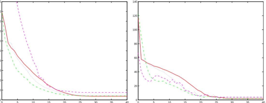
0 5 10 15 20 25 30 35 40 150 160 170 180 190 200 210 220 230 240 250 0 5 10 15 20 25 30 35 40 0 20 40 60 80 100 120 140

Figure 7. Convergence histories of the criterion

j

(Ω) (left) and of the angle

θ

ex-pressed in degrees (right), for the four examples represented by a solid, dotted,

dash-dotted and dashed line, respectively.

level-set function is defined on a mesh of 1658 nodes and the elasticity analysis

is performed on a mesh of 6515 nodes (one level refinement). Figures 9 and 10

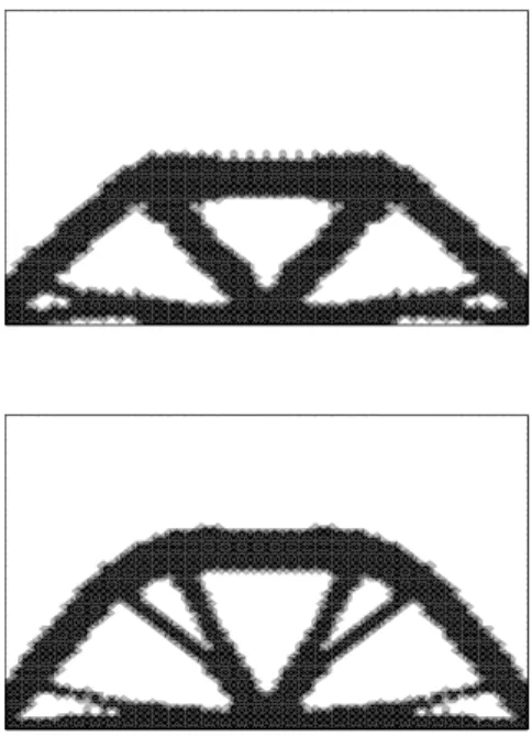
show the result obtained with the trivial full domain initialization.

Figure 8. Boundary conditions for the bridge.

4.3

Mast

This example is taken from [3]. The working domain is T-shaped with the

vertical branch of size 2

×

4 and the horizontal one of size 4

×

2. A vertical

(16)

Figure 9. Iterations 6 and 30 of the bridge with

ψ

initialized by a negative constant.

0 5 10 15 20 25 30 35 40 45 50 55 60 65 70 75 80 85 0 5 10 15 20 25 30 0 20 40 60 80 100 120

Figure 10. Convergences histories of the criterion

j

θ

expressed in degrees (right) for the bridge.

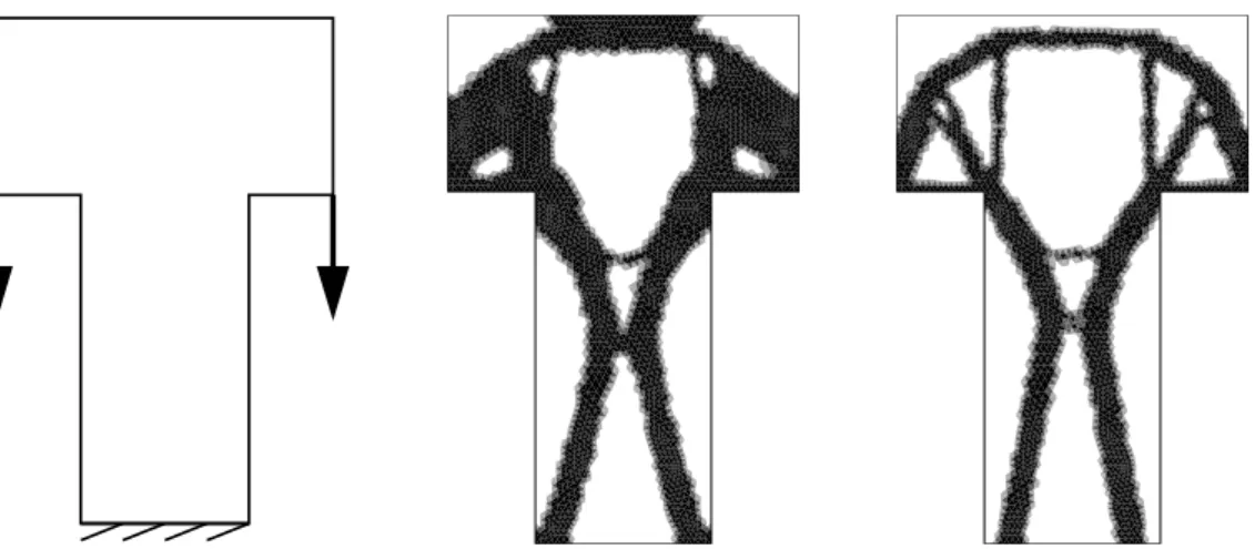
unitary force is applied at the bottom corners of the horizontal branch and

the bottom of the vertical branch is fixed. The Lagrange multiplier is

`

=

15. A mesh with 4265 nodes is used for the elasticity analysis as well as for

representing the level-set function. The results are displayed on Figures 11

and 12. Very similar results are obtained by applying a one level filter.

4.4

Gripping mechanism

This is again a classical test case that has been treated for instance in [5,3]. The

location of the external forces is split into two regions Γ

F1

and Γ

F2

supporting

a load

ϕ

1

and

ϕ

2

, respectively (see Fig. 13). Free boundary conditions are

prescribed elsewhere. Unlike all previous examples, we are not interested here

in compliance minimization. We still consider a criterion

j

(Ω) of the form (2),

(17)

Figure 11. Boundary conditions and iterations 10 and 40 of the mast with

ψ

initial-ized by a negative constant.

0 5 10 15 20 25 30 35 40 140 160 180 200 220 240 260 280 0 5 10 15 20 25 30 35 40 0 20 40 60 80 100 120

Figure 12. Convergences histories of the criterion

j

θ

expressed in degrees (right) for the mast.

but for the functional

J(u) =

β

1

Z

ΓF₁

ϕ

1

.uds

+

β

2

Z

ΓF₂

ϕ

2

.uds,

with fixed coefficients

β

1

and

β

2

. In this case, the evaluation of the topological

gradient requires the solution of an adjoint problem. Figure 14 shows the

results of two computations performed with the following sets of parameters:

ϕ

1

=

−

10n

(n

denoting the outward unit normal),

ϕ

2

=

−

n,

β

1

= 0.1,

β

2

= 1,

`

= 0.3 for the first configuration (left),

ϕ

1

=

−

n,

ϕ

2

=

−

10n,

β

1

= 1,

β

2

= 0.1,

`

= 0.3 for the second one (right). Since thin structures are needed to get an

efficient mechanism, we use a fine mesh of 8731 nodes without filtering.

5

A multidisciplinary problem: optimization of a ceramic filter

5.1

Introduction

This problem concerns the optimal design of a certain class of waste water

ceramic filters, which basically operate as follows (see Fig. 15). Thanks to an

(18)

Γ

F2

F1

Figure 13. Boundary conditions for the gripping mechanism.

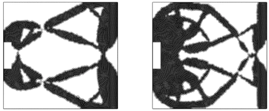
Figure 14. Obtained designs after 30 iterations for the gripping mechanism in two

different configurations (

ψ

is initialized by a negative constant).

appropriate housing, the waste water is distributed all around the external

surface of the filter, which has the shape of an elliptic cylinder. Due to high

pressure gradients, the fluid crosses the porous medium and the filtered water

reaches the top of the device through some vertical channel(s). The issue

con-sists in determining the number, the location and the shape of these channels

such that they allow for a maximal flow rate provided that the structure does

not break on the effect of the pressure.

(19)

5.2

Mathematical model

We consider a 2D model by taking an horizontal cross-section. Therefore our

computational domain

D

is an ellipse. To simplify the writing, since the

bound-ary conditions on the external border are everywhere of Neumann type, we

denote by Γ the boundary of

D.

The behavior of the fluid is modeled by the Stokes-Brinkman system [16]:











−

η∆U

Ω

+

η

˜

k

−1

U

Ω

+

∇

p

Ω

= 0

in

D,

div

U

Ω

= ˜

s

in

D,

η

∇

U

Ω

.n

−

p

Ω

n

=

−

p

out

n

on Γ,

(17)

where

U

Ω

and

p

Ω

stand for the velocity and the pressure fields,

p

out

is the

outside pressure,

η

is the dynamic viscosity of the fluid and the tilde quantities

are defined by

˜

k

−1

=











k

−1

in Ω,

0

in

D

\

Ω,

s

˜

=











0 in Ω,

s

in

D

\

Ω.

The letter

k

denotes the permeability of the porous medium and

s

is a sink

term simulating the vertical flow. In our model,

s

is a prescribed negative

constant.

The displacement field

u

Ω

of the structure is computed through the following

equations, with the same notations as in (5):











−

div ( ˜

αAe(u

Ω

)) =

−∇

p

Ω

in

D,

(Ae(u

Ω

))n

−

p

Ω

n

=

−

p

out

n

on Γ.

(18)

Since

p

out

is supposed to be constant, we remark that we obtain homogeneous

boundary conditions in (17) and (18) by taking as new variable the difference

p

0

Ω

=

p

Ω

−

p

out

. Assuming this change of variable has been done, we consider

henceforth that

p

out

= 0.

We still consider a criterion

j(Ω) to be minimized of the form (2) with the

compliance

J(u, p) =

Z

Γ

pu.nds

−

Z

D

∇

p.udx

=

Z

D

p

div

udx.

(20)

In our model, the additional term

`

|

Ω

|

is a decreasing function of the flow rate,

which we want to maximize. It also accounts for the price of the structure.

(The material used for such filters is indeed very expensive.)

5.3

Topological sensitivity

The variational formulation of the boundary value problem (17), (18) reads:

find (U

Ω

, p

Ω

, u

Ω

)

∈

H

1

(D)

2

×

L

2

(D)

×

H

1

(D)

2

such that











c

Ω

(U

Ω

, V

) +

d(V, p

Ω

) = 0

∀

V

∈

(H

1

(D))

2

,

d(U

Ω

, q) =

s

Ω

(q)

∀

q

∈

L

2

(D),

a

Ω

(u

Ω

, v) =

d(v, p

Ω

)

∀

v

∈

(H

1

(D))

2

,

(19)

with the bilinear forms

c

Ω

(U, V

) =

η

Z

D

(

∇

U

:

∇

V

+ ˜

k

−1

U.V

)dx,

d(V, p) =

Z

D

p

div

V dx,

a

Ω

(u, v) =

Z

D

˜

αAe(u) :

e(v)dx,

and the linear form

s

Ω

(q) =

Z

D

˜

sqdx.

We introduce the Lagrangian

L

Ω

(U, V, p, q, u, v) =

J

(u, p)+`

|

Ω

|

+c

Ω

(U, V

)+d(V, p)+d(U, q)

−

s

Ω

(q)+a

Ω

(u, v)

−

d(v, p).

Thanks to (19) it comes

j(Ω) =

L

Ω

(U

Ω

, V, p

Ω

, q, u

Ω

, v)

∀

V, q, v.

Although neither the Lagrangian

L

Ω

nor the fields

U

Ω

,

p

Ω

and

u

Ω

are

differen-tiable with respect to a variation of topology, the composition of the sensitivity

formula as well as the relevant adjoint states can be exactly obtained by

ap-plying formally the rules of differential calculus (see

e.g.

[19]). Within this

framework, we have for a domain perturbation

τ:

Dj(Ω)τ

=

∂

Ω

L

Ω

(U

Ω

, V, p

Ω

, q, u

Ω

, v)τ

+

∂

U

L

Ω

(U

Ω

, V, p

Ω

, q, u

Ω

, v

)(DU

Ω

τ

)

(21)

Let us study each term successively, starting by the last one. It follows from

the bilinearity of

J

and

a

Ω

that, for any

δ

u

,

∂

u

L

Ω

(U

Ω

, V, p

Ω

, q, u

Ω

, v)δ

u

=

J(δ

u

, p

Ω

) +

a

Ω

(δ

u

, v).

As

v

is arbitrary, we choose

v

=

v

Ω

=

−

u

Ω

which, as a consequence of (19)

together with the symmetry of

a

Ω

and the identity

J

=

d, permits to cancel

the above expression. Then we have

∂

p

L

Ω

(U

Ω

, V, p

Ω

, q, u

Ω

, v

Ω

)δ

p

=

J(u

Ω

, δ

p

) +

d(V, δ

p

)

−

d(v

Ω

, δ

p

) =

d(2u

Ω

+

V, δ

p

),

∂

U

L

Ω

(U

Ω

, V, p

Ω

, q, u

Ω

, v

Ω

)δ

U

=

c

Ω

(δ

U

, V

) +

d(δ

U

, q).

Again, the two above expressions can be canceled by an adequate choice of

V

and

q, namely by choosing them as the solution of the adjoint problem:











−

η∆V

Ω

+

η

k

˜

−1

V

Ω

+

∇

q

Ω

= 0

in

D,

div

V

Ω

=

−

2 div

u

Ω

in

D,

η

∇

V

Ω

.n

−

q

Ω

n

= 0

on Γ.

(20)

Finally it remains

Dj(Ω)τ

=

∂

Ω

L

Ω

(U

Ω

, V

Ω

, p

Ω

, q

Ω

, u

Ω

, v

Ω

)τ

=

`∂

Ω

|

Ω

|

τ

+

∂

Ω

c

Ω

(U

Ω

, V

Ω

)τ

−

∂

Ω

s

Ω

(q

Ω

)τ

+

∂

Ω

a

Ω

(u

Ω

, v

Ω

)τ.

Let us now consider the case where the perturbation

τ

consists in adding or

removing in Ω a small disc

B

(x, ρ). The sense of that perturbation is again

represented by a variable

δ

according to (8). Then in the above expression the

derivatives with respect to the domain stand for topological derivatives. The

first and the third terms come straightforwardly. The last one has been

ex-plicited in Subsection 3.1. The second one can be easily derived by proceeding

like in [8]. Altogether we obtain

Dj

(Ω)τ

=

|

B(x, ρ)

|

g(x)δ

˜

with

˜

g

=

η

˜

k

−1

U

Ω

.V

Ω

+ ˜

sq

Ω

+ ˜

g

struc

(u

Ω

, v

Ω

).

The function ˜

g

struc

is given by (9).

5.4

Numerical results

The numerical data used are

η

= 0.01,

k

−1

= 5000 and

s

=

−

1. The elastic

(22)

of ceramics on the border of the domain is imposed in order to guarantee a

sufficient filtering efficiency. It corresponds to 15% of the external radius in

elliptic coordinates. In the cost functional, the Lagrange multiplier

`

= 100 is

chosen.

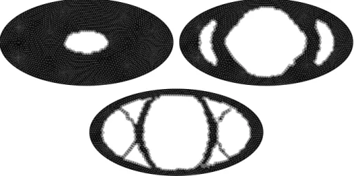
Figures 16, 17, 18 and 19 show the results of two computations, corresponding

to two different shapes of the working domain

D. In order to avoid starting

on a local extremum, the level-set function is initialized in such a way that Ω

0

is

D

deprived of a small elliptic hole located around its center. For those two

examples, 801 design variables are handled and the meshes used to solve the

PDE consist of 3105 and 3073 nodes, respectively. The slight dissymmetries

on the obtained designs with respect to the main axes are entirely due to the

dissymmetry of the mesh. As a postprocessing step towards the validation of

these structures, we have represented the map of the highest principal stress

which provides a good breaking criterion for ceramics. Indeed, the real problem

is rather complicated, involving several criteria and several parameters. We

have adopted a standard approach in engineering consisting in running an

optimization procedure for a chosen criterion and certain fixed parameters

(like the shape of the ellipse or the Lagrange multiplier). It must be checked

afterwards that all constraints are satisfied by the obtained solution.

Figure 16. Initial guess and iterations 3 and 20 of the filter with semi-axes 1

×

0

.

5.

(23)

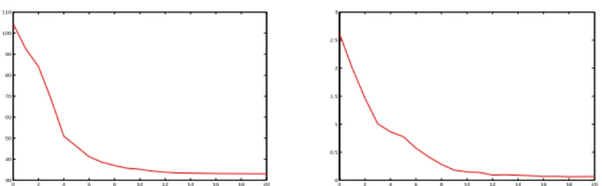
0 2 4 6 8 10 12 14 16 18 20 30 40 50 60 70 80 90 100 110 0 2 4 6 8 10 12 14 16 18 20 0 0.5 1 1.5 2 2.5 3

Figure 18. Convergences histories of the criterion

j

θ

expressed in degrees (right) for the filter.

Figure 19. Iteration 20 of the filter with semi-axes 2

×

0

.

5: design (left) and highest

principal stress (right).

6

Conclusion

We have proposed a new algorithm for simultaneous topology and shape

opti-mization, which has some advantages compared to other level-set based

meth-ods.

•

Satisfactory results are obtained without any a priori on the topology (in

general, the best results are obtained with the trivial full domain

initializa-tion). For classical examples, they are very similar to the results obtained

in [5].

•

The algorithm derives from an unique evolution equation which does not

involve any arbitrary parameter. We recall that in [3] the solution of the

Hamilton-Jacobi equation, the reinitialization process and the nucleation

process have to be performed alternatively with manually chosen

frequen-cies, and that in [12] the corrective term added to the Hamilton-Jacobi

equation is controlled by a coefficient to be adjusted by heuristics.

•

The level-set function has a meaning after convergence (

i.e.

at the stationary

point of the evolution equation in the continuous model): it is the normalized

topological gradient. Therefore the corresponding design satisfies necessary

topological optimality conditions, which are even sufficient in a certain class

of perturbations.

•

We have distinguished the mesh representing the geometry and the mesh

used to solve the PDE. This enables to have a moderate number of degrees

of freedom for the shape whereas the solution remains computed accurately.

We point out that this accuracy as well as the efficiency could be improved

by the use of a specific fast solver (see

e.g.

[24]).

However, there remain (at least) the following inconveniences. As mentioned

in [3], non-relaxed topology optimization problems are generally subject to

(24)

local minima and our filtering technique recalled above cures only partially

this phenomenon. Another weakness concerns the choice of the Lagrange

mul-tiplier. We always considered it as fixed from the beginning and so far we

have no way to update it during the optimization process in connection with

a given volume constraint.

Acknowledgements.

The authors are grateful to Oleg Iliev for his valuable

help concerning Section 5.

References

[1]

G. Allaire

,

Shape optimization by the homogenization method, Springer

Verlag, New York, 2001.

[2]

G. Allaire, E. Bonnetier, G. Francfort and F. Jouve

,

Shape

optimization by the homogenization method, Numer. Math. 76, pp. 27-68,

1997.

[3]

G. Allaire, F. de Gournay, F. Jouve and A.-M. Toader

,

Structural

optimization using topological and shape sensitivity analysis via a level-set

method, Internal report no. 555, CMAP Ecole Polytechnique, 2004.

[4]

G. Allaire, F. Jouve

,

A level-set method for vibration and multiple loads

structural optimization, Comput. Methods Appl. Mech. Engrg. 194, pp.

3269-3290, 2005.

[5]

G. Allaire, F. Jouve and A.-M. Toader

,

Structural optimization using

sensitivity analysis and a level-set method, J. Comp. Phys. 194, pp. 363-393,

2004.

[6]

G. Allaire and R. Kohn

,

Optimal design for minimum weight and

compliance in plane stress using extremal microstructures, European Journal

of Mechanics, A/Solids, 12(6), pp. 839-878, 1993.

[7]

H. Ammari, H. Kang

,

Reconstruction of small inhomogeneities from

boundary measurements, Lecture Notes in Mathematics 1846, Springer, 2004.

[8]

S. Amstutz, N. Dominguez and B. Samet

,

Sensitivity analysis with

respect to the insertion of small inhomogeneities, proceedings of ECCOMAS

2004.

[9]

M. Bendsoe, N. Kikuchi

,

Generating optimal topologies in structural

design using an homogenization method, Comput. Methods Appl. Engrg. 71,

pp. 197-224, 1988.

[10]

M. Bendsoe, O. Sigmund

,

Topology optimization. Theory, Methods and

Applications, Springer Verlag, New York, 2003.

(25)

[11]

M. Burger

,

A framework for the construction of level-set methods for shape

optimization and reconstruction, Interfaces and Free Boundaries 5, pp.

301-329, 2003.

[12]

M. Burger, B. Hackl and W. Ring

,

Incorporating topological derivatives

into level-set methods, J. Comp. Phys. 194(1), pp. 344-362, 2004.

[13]

J. C´

ea

,

Conception optimale ou identification de forme, calcul rapide de la

d´

eriv´

ee directionnelle de la fonction coˆ

ut, M.A.A.N., 20(3), pp. 371-402, 1986.

[14]

F.

Daoud,

N.

Camprubi

and

K.-U.

Bletzinger

,

Filtering and regularization techniques in shape optimization with CAD-free

parametrization, Lehrstuhl f¨

ur Statik, TU M¨

unchen.

[15]

S. Garreau, Ph. Guillaume, M. Masmoudi

,

The topological Asymptotic

for PDE systems: the elasticity case, SIAM J. Control Optim. 39(6), pp.

1756-1778, 2001.

[16]

O. Iliev and V. Laptev

,

On numerical simulation of flow through oil

filters, Comput. Visual. Sci. 6, pp. 139-146, 2004.

[17]

J.

Jacobsen,

N.

Olhoff

and

E.

Ronholt

,

Generalized

shape

optimization of three-dimensional structures using materials with optimum

microstructures, Technical report, Institute of Mechanical Engineering,

Aalborg University, 1996.

[18]

C. Kane and M. Schoenauer

,

Topological optimum design using genetic

algorithms, Control and Cybernetics 25, pp. 1059-1088, 1996.

[19]

M. Masmoudi

,

The Toplogical Asymptotic, Computational Methods for

Control Applications, R. Glowinski, H. Kawarada and J. Periaux eds.,

GAKUTO Internat. Ser. Math. Sci. Appl. Vol. 16, pp. 53-72, 2001.

[20]

F. Murat and J. Simon

,

Sur le contrˆ

ole par un domaine g´

eom´

etrique, PhD

thesis, Paris, 1976.

[21]

S.

Osher

and

F.

Santosa

,

Level-set

methods

for

optimization

problems involving geometry and constraints: frequencies of a two-density

inhomogeneous drum, J. Comp. Phys. 171, pp. 272-288, 2001.

[22]

S. Osher and J.A. Sethian

,

Front propagating with curvature dependent

speed: algorithms based on Hamilton-Jacobi formulations, J. Comp. Phys. 78,

pp. 12-49, 1988.

[23]

A. Schumacher, V.V. Kobolev and H.A. Eschenauer

,

Bubble method

for topology and shape optimization of structures, Journal of structural

optimization no. 8, pp. 42-51, 1994.

[24]

J. Sethian and A. Wiegmann

,

Structural boundary design via level-set

and immersed interface method, J. Comp. Phys. 163, pp. 489-528, 2000.

[25]

J. Sokolowski and A. Zochowski

,

On the topological derivative in shape

(26)

[26]

J. Sokolowski and J.-P. Zolesio

,

Introduction to shape optimization:

shape sensitivity analysis, Springer Series in Computational Mathematics vol.

10, Springer, Berlin, 1992.

[27]

M.Y. Wang, X. Wang and D. Guo

,

A level-set method for structural

topology optimization, Comput. Meth. Appl. Mech. Engrg. 192, pp. 227-246,

2003.

[28]

X. Wang, M. Yulin and M.Y. Wang

,

Incorporating topological derivatives

into level-set methods for structural topology optimization, Optimal shape

design and modeling, T. Lewinski et al. eds, pp. 145-157, Polish Academy of

Sciences, Warsaw, 2004.

(27)

Published reports of the

Fraunhofer ITWM

The PDF-ﬁ les of the following reports

are available under:

www.itwm.fraunhofer.de/de/

zentral__berichte/berichte

1. D. Hietel, K. Steiner, J. Struckmeier

A Finite - Volume Particle Method for

Compressible Flows

We derive a new class of particle methods for ser va tion laws, which are based on numerical ﬂ ux functions to model the in ter ac tions between moving particles. The der i va tion is similar to that of classi-cal Finite-Volume meth ods; except that the ﬁ xed grid structure in the Fi nite-Volume method is sub sti tut ed by so-called mass pack ets of par ti cles. We give some numerical results on a shock wave solution for Burgers equation as well as the well-known one-dimensional shock tube problem.

(19 pages, 1998)

2. M. Feldmann, S. Seibold

Damage Diagnosis of Rotors: Application

of Hilbert Transform and

Multi-Hypothe-sis Testing

In this paper, a combined approach to damage diag-nosis of rotors is proposed. The intention is to employ signal-based as well as model-based procedures for an im proved detection of size and location of the damage. In a fi rst step, Hilbert transform signal processing niques allow for a computation of the signal envelope and the in stan ta neous frequency, so that various types of non-linearities due to a damage may be identifi ed and clas si fi ed based on measured response data. In a second step, a multi-hypothesis bank of Kalman Filters is employed for the detection of the size and location of the damage based on the information of the type of damage pro vid ed by the results of the Hilbert trans-form.

Keywords: Hilbert transform, damage diagnosis, Kal-man ﬁ ltering, non-linear dynamics

(23 pages, 1998)

3. Y. Ben-Haim, S. Seibold

Robust Reliability of Diagnostic

Multi-Hypothesis Algorithms: Application to

Rotating Machinery

Damage diagnosis based on a bank of Kalman fi l-ters, each one conditioned on a specifi c hypothesized system condition, is a well recognized and powerful diagnostic tool. This multi-hypothesis approach can be applied to a wide range of damage conditions. In this paper, we will focus on the diagnosis of cracks in rotating machinery. The question we address is: how to optimize the multi-hypothesis algorithm with respect to the uncertainty of the spatial form and location of cracks and their re sult ing dynamic effects. First, we formulate a measure of the re li abil i ty of the diagnos-tic algorithm, and then we dis cuss modifi cations of the diagnostic algorithm for the max i mi za tion of the reliability. The reliability of a di ag nos tic al go rithm is measured by the amount of un cer tain ty con sis tent with no-failure of the diagnosis. Un cer tain ty is quan ti ta tive ly represented with convex models.

Keywords: Robust reliability, convex models, Kalman ﬁ l ter ing, multi-hypothesis diagnosis, rotating machinery, crack di ag no sis

(24 pages, 1998)

4. F.-Th. Lentes, N. Siedow

Three-dimensional Radiative Heat Transfer

in Glass Cooling Processes

Since the ex act solution would require super-computer ca pa bil i ties we concentrate on approximate solu-tions with a high degree of accuracy. The following approaches are stud ied: 3D diffusion approximations and 3D ray-tracing meth ods.

(23 pages, 1998)

5. A. Klar, R. Wegener

A hierarchy of models for multilane

vehicular trafﬁ c

Part I: Modeling

In the present paper multilane models for vehicular traffi c are considered. A mi cro scop ic multilane model based on reaction thresholds is developed. Based on this mod el an Enskog like kinetic model is developed. In particular, care is taken to incorporate the correla-tions between the ve hi cles. From the kinetic model a fl uid dynamic model is de rived. The macroscopic coef-fi cients are de duced from the underlying kinetic model. Numerical simulations are presented for all three levels of description in [10]. More over, a comparison of the results is given there.

(23 pages, 1998)

Part II: Numerical and stochastic

investigations

In this paper the work presented in [6] is continued. The present paper contains detailed numerical inves-tigations of the models developed there. A numerical method to treat the kinetic equations obtained in [6] are presented and results of the simulations are shown. Moreover, the stochastic correlation model used in [6] is described and investigated in more detail. (17 pages, 1998)

6. A. Klar, N. Siedow

Boundary Layers and Domain De com po

si tsion for Radsiatsive Heat Transfer and Dsif fu

sion Equa tions: Applications to Glass Man u

-fac tur ing Processes

In this paper domain decomposition methods for ra di a tive transfer problems including conductive heat transfer are treated. The paper focuses on semi-trans-parent ma te ri als, like glass, and the associated condi-tions at the interface between the materials. Using asymptotic anal y sis we derive conditions for the cou-pling of the radiative transfer equations and a diffu-sion approximation. Several test cases are treated and a problem appearing in glass manufacturing processes is computed. The results clearly show the advantages of a domain decomposition ap proach. Accuracy equivalent to the solution of the global radiative transfer solu-tion is achieved, whereas com pu ta solu-tion time is strongly reduced.

(24 pages, 1998)

7. I. Choquet

Heterogeneous catalysis modelling and

numerical simulation in rariﬁ ed gas ﬂ ows

Part I: Coverage locally at equilibrium

A new approach is proposed to model and simulate nu mer i cal ly heterogeneous catalysis in rareﬁ ed gas ﬂ ows. It is developed to satisfy all together the follow-ing points:

1) describe the gas phase at the microscopic scale, as required in rareﬁ ed ﬂ ows,

2) describe the wall at the macroscopic scale, to avoid prohibitive computational costs and consider not only crystalline but also amorphous surfaces,

3) reproduce on average macroscopic laws correlated with experimental results and

4) derive analytic models in a systematic and exact way. The problem is stated in the general framework of a non static ﬂ ow in the vicinity of a catalytic and non porous surface (without aging). It is shown that the exact and systematic resolution method based on the Laplace trans form, introduced previously by the author to model col li sions in the gas phase, can be extended to the present problem. The proposed approach is applied to the mod el ling of the Eley Rideal

extended to the general case of sev er al atomic species. Numerical calculations show that the models derived in this way reproduce with accuracy be hav iors observed experimentally.

(24 pages, 1998)

8. J. Ohser, B. Steinbach, C. Lang

Efﬁ cient Texture Analysis of Binary Images

A new method of determining some characteristics of binary images is proposed based on a special linear fi l ter ing. This technique enables the estimation of the area fraction, the specifi c line length, and the specifi c integral of curvature. Furthermore, the specifi c length of the total projection is obtained, which gives detailed information about the texture of the image. The in fl u ence of lateral and directional resolution depend-ing on the size of the applied fi lter mask is discussed in detail. The technique includes a method of increasing di rec tion al resolution for texture analysis while keeping lateral resolution as high as possible.

(17 pages, 1998)

9. J. Orlik

Homogenization for viscoelasticity of the

integral type with aging and shrinkage

A multi phase composite with periodic distributed in clu sions with a smooth boundary is considered in this con tri bu tion. The composite component materials are sup posed to be linear viscoelastic and aging (of the non-convolution integral type, for which the Laplace form with respect to time is not effectively ap pli ca ble) and are subjected to isotropic shrinkage. The free shrinkage deformation can be considered as a fi cti-tious temperature deformation in the behavior law. The pro ce dure presented in this paper proposes a way to de ter mine average (effective homogenized) viscoelastic and shrinkage (temperature) composite properties and the homogenized stress fi eld from known properties of the components. This is done by the extension of the as ymp tot ic homogenization technique known for pure elastic non homogeneous bodies to the non homo-geneous thermo viscoelasticity of the integral non con-volution type. Up to now, the homogenization theory has not covered viscoelasticity of the integral type. Sanchez Palencia (1980), Francfort & Suquet (1987) (see [2], [9]) have considered homogenization for vis coelas -tic i ty of the differential form and only up to the fi rst de riv a tive order. The integral modeled viscoelasticity is more general then the differential one and includes almost all known differential models. The homogeni-zation pro ce dure is based on the construction of an asymptotic so lu tion with respect to a period of the composite struc ture. This reduces the original problem to some auxiliary bound ary value problems of elastic-ity and viscoelasticelastic-ity on the unit periodic cell, of the same type as the original non-homogeneous problem. The existence and unique ness results for such problems were obtained for kernels satisfying some constrain conditions. This is done by the extension of the Volterra integral operator theory to the Volterra operators with respect to the time, whose 1 ker nels are space linear operators for any fi xed time vari ables. Some ideas of such approach were proposed in [11] and [12], where the Volterra operators with kernels depending addi-tionally on parameter were considered. This manuscript delivers results of the same nature for the case of the space operator kernels.

(20 pages, 1998)

10. J. Mohring

Helmholtz Resonators with Large Aperture

The lowest resonant frequency of a cavity resona-tor is usually approximated by the clas si cal Helmholtz formula. However, if the opening is rather large and the front wall is narrow this formula is no longer valid. Here we present a correction which is of third or der in the ratio of the di am e ters of aperture and cavity. In addition to the high accuracy it allows to estimate the damping due to ra di a tion. The result is found by apply-ing the method of matched asymptotic expansions. The correction contains form factors de scrib ing the shapes of opening and cavity. They are computed for a

(28)

num-11. H. W. Hamacher, A. Schöbel

On Center Cycles in Grid Graphs

Finding “good” cycles in graphs is a problem of great in ter est in graph theory as well as in locational analy-sis. We show that the center and median problems are NP hard in general graphs. This result holds both for the vari able cardinality case (i.e. all cycles of the graph are con sid ered) and the fi xed cardinality case (i.e. only cycles with a given cardinality p are feasible). Hence it is of in ter est to investigate special cases where the problem is solvable in polynomial time. In grid graphs, the variable cardinality case is, for in stance, trivially solvable if the shape of the cycle can be chosen freely. If the shape is fi xed to be a rectangle one can ana-lyze rectangles in grid graphs with, in sequence, fi xed di men sion, fi xed car di nal i ty, and vari able cardinality. In all cases a complete char ac ter iza tion of the opti-mal cycles and closed form ex pres sions of the optiopti-mal ob jec tive values are given, yielding polynomial time algorithms for all cas es of center rect an gle prob lems. Finally, it is shown that center cycles can be chosen as rectangles for small car di nal i ties such that the center cy cle problem in grid graphs is in these cases plete ly solved.

(15 pages, 1998)

12. H. W. Hamacher, K.-H. Küfer

Inverse radiation therapy planning -

a multiple objective optimisation ap proach

For some decades radiation therapy has been proved successful in cancer treatment. It is the major task of clin i cal radiation treatment planning to realize on the one hand a high level dose of radiation in the cancer tissue in order to obtain maximum tumor control. On the other hand it is obvious that it is absolutely neces-sary to keep in the tissue outside the tumor, particularly in organs at risk, the unavoidable radiation as low as possible.

No doubt, these two objectives of treatment planning - high level dose in the tumor, low radiation outside the

tumor - have a basically contradictory nature. Therefore, it is no surprise that inverse mathematical models with dose dis tri bu tion bounds tend to be infeasible in most cases. Thus, there is need for approximations pro mis ing between overdosing the organs at risk and un der dos ing the target volume.

Differing from the currently used time consuming it er a tive approach, which measures de vi a tion from an ideal (non-achievable) treatment plan us ing re cur sive ly trial-and-error weights for the organs of in ter est, we go a new way trying to avoid a priori weight choic es and con sid er the treatment planning problem as a mul-tiple ob jec tive linear programming problem: with each organ of interest, target tissue as well as organs at risk, we as so ci ate an objective function measuring the maxi-mal de vi a tion from the prescribed doses.

We build up a data base of relatively few efﬁ cient so lu tions rep re sent ing and ap prox i mat ing the vari-ety of Pare to solutions of the mul ti ple objective linear programming problem. This data base can be easily scanned by phy si cians look ing for an ad e quate treat-ment plan with the aid of an appropriate on line tool. (14 pages, 1999)

13. C. Lang, J. Ohser, R. Hilfer

On the Analysis of Spatial Binary Images

This paper deals with the characterization of mi cro -scop i cal ly heterogeneous, but macro-scopically homo-geneous spatial structures. A new method is presented which is strictly based on integral-geometric formulae such as Crofton’s intersection formulae and Hadwiger’s recursive deﬁ nition of the Euler number. The corre-sponding al go rithms have clear advantages over other techniques. As an example of application we con-sider the analysis of spatial digital images produced by means of Computer Assisted Tomography.

(20 pages, 1999)

14. M. Junk

On the Construction of Discrete Equilibrium

Distributions for Kinetic Schemes

ciples are also applied to the construction of Chapman Enskog dis tri bu tions which are used in Kinetic Schemes for com press ible Navier-Stokes equations.

(24 pages, 1999)

15. M. Junk, S. V. Raghurame Rao

A new discrete velocity method for

Navier-Stokes equations

The relation between the Lattice Boltzmann Method, which has recently become popular, and the Kinetic Schemes, which are routinely used in Computational Flu id Dynamics, is explored. A new discrete veloc-ity model for the numerical solution of Navier-Stokes equa tions for incompressible ﬂ uid ﬂ ow is presented by com bin ing both the approaches. The new scheme can be interpreted as a pseudo-compressibility method and, for a particular choice of parameters, this interpretation carries over to the Lattice Boltzmann Method. (20 pages, 1999)

16. H. Neunzert

Mathematics as a Key to Key Technologies

The main part of this paper will consist of examples, how mathematics really helps to solve industrial lems; these examples are taken from our Institute for Industrial Mathematics, from research in the Tech no-math e mat ics group at my university, but also from ECMI groups and a company called TecMath, which orig i nat ed 10 years ago from my university group and has already a very suc cess ful history.

(39 pages (4 PDF-Files), 1999)

17. J. Ohser, K. Sandau

Considerations about the Estimation of the

Size Distribution in Wicksell’s Corpuscle

Prob lem

Wicksell’s corpuscle problem deals with the estima-tion of the size distribuestima-tion of a populaestima-tion of particles, all hav ing the same shape, using a lower dimensional sampling probe. This problem was originary formulated for particle systems occurring in life sciences but its solution is of actual and increasing interest in materials science. From a mathematical point of view, Wicksell’s problem is an in verse problem where the interest-ing size distribution is the unknown part of a Volterra equation. The problem is often regarded ill-posed, because the structure of the integrand implies unsta-ble numerical solutions. The ac cu ra cy of the numeri-cal solutions is considered here using the condition number, which allows to compare different numerical methods with different (equidistant) class sizes and which indicates, as one result, that a ﬁ nite section thickness of the probe reduces the numerical problems. Furthermore, the rel a tive error of estimation is com-puted which can be split into two parts. One part con-sists of the relative dis cret i za tion error that increases for in creas ing class size, and the second part is related to the rel a tive statistical error which increases with decreasing class size. For both parts, upper bounds can be given and the sum of them indicates an optimal class width depending on some speciﬁ c constants. (18 pages, 1999)

18. E. Carrizosa, H. W. Hamacher, R. Klein,

S. Nickel

Solving nonconvex planar location

prob-lems by ﬁ nite dominating sets

It is well-known that some of the classical location prob lems with polyhedral gauges can be solved in poly no mi al time by fi nding a fi nite dominating set, i. e. a fi nite set of candidates guaranteed to contain at least one op ti mal location.

In this paper it is ﬁ rst established that this result holds for a much larger class of problems than currently sid ered in the literature. The model for which this result can be prov en includes, for instance, location prob lems with at trac tion and repulsion, and location-al lo ca tion prob lems.

Next, it is shown that the ap prox i ma tion of general gaug es by polyhedral ones in the objective function of

al go rithm. Both of these approaches lead - for ﬁ xed epsilon - to polyno mial ap prox i ma tion algorithms with accuracy epsilon for solving the general model sid ered in this paper.

Keywords: Continuous Location, Polyhedral Gauges, Finite Dom i nat ing Sets, Approximation, Sandwich Al go -rithm, Greedy Algorithm

(19 pages, 2000)

19. A. Becker

A Review on Image Distortion Measures

Within this paper we review image distortion mea-sures. A distortion measure is a criterion that assigns a “quality number” to an image. We distinguish between math e mat i cal distortion measures and those distortion mea sures in-cooperating a priori knowledge about the im ag ing devices ( e. g. satellite images), image pro-cessing al go rithms or the human physiology. We will consider rep re sen ta tive examples of different kinds of distortion mea sures and are going to discuss them.

Keywords: Distortion measure, human visual system

(26 pages, 2000)

20. H. W. Hamacher, M. Labbé, S. Nickel,

T. Sonneborn

Polyhedral Properties of the Uncapacitated

Multiple Allocation Hub Location Problem

We examine the feasibility polyhedron of the un ca -pac i tat ed hub location problem (UHL) with multiple al lo ca tion, which has applications in the ﬁ elds of air passenger and cargo transportation, telecommuni-cation and postal delivery services. In particular we determine the di men sion and derive some classes of facets of this polyhedron. We develop some general rules about lifting facets from the uncapacitated facility location (UFL) for UHL and pro ject ing facets from UHL to UFL. By applying these rules we get a new class of facets for UHL which dom i nates the inequalities in the original formulation. Thus we get a new formulation of UHL whose constraints are all facet–deﬁ ning. We show its superior computational per for mance by benchmark-ing it on a well known data set.

Keywords: integer programming, hub location, facility location, valid inequalities, facets, branch and cut

(21 pages, 2000)

21. H. W. Hamacher, A. Schöbel

Design of Zone Tariff Systems in Public

Trans por ta tion

Given a public transportation system represented by its stops and direct connections between stops, we con-sider two problems dealing with the prices for the cus-tomers: The fare problem in which subsets of stops are already aggregated to zones and “good” tariffs have to be found in the existing zone system. Closed form solutions for the fare problem are presented for three objective functions. In the zone problem the design of the zones is part of the problem. This problem is NP hard and we there fore propose three heuristics which prove to be very successful in the redesign of one of Germany’s trans por ta tion systems.

(30 pages, 2001)

22. D. Hietel, M. Junk, R. Keck, D. Teleaga

The Finite-Volume-Particle Method for

Conservation Laws

In the Finite-Volume-Particle Method (FVPM), the weak formulation of a hyperbolic conservation law is dis cretized by restricting it to a discrete set of test func-tions. In con trast to the usual Finite-Volume approach, the test func tions are not taken as characteristic func-tions of the con trol volumes in a spatial grid, but are chosen from a par ti tion of unity with smooth and overlapping partition func tions (the particles), which can even move along pre - scribed velocity ﬁ elds. The information exchange be tween particles is based on standard numerical ﬂ ux func tions. Geometrical infor-mation, similar to the surface area of the cell faces in the Finite-Volume Method and the cor re spond ing normal directions are given as integral quan ti ties of the

(29)

23. T. Bender, H. Hennes, J. Kalcsics,

M. T. Melo, S. Nickel

Location Software and Interface with GIS

and Supply Chain Management