Full Terms & Conditions of access and use can be found at
http://www.tandfonline.com/action/journalInformation?journalCode=rquf20
Download by: [Imperial College London Library] Date: 23 September 2016, At: 06:37
Quantitative Finance
ISSN: 1469-7688 (Print) 1469-7696 (Online) Journal homepage: http://www.tandfonline.com/loi/rquf20
Gaussian process-based algorithmic trading
strategy identification
Steve Y. Yang, Qifeng Qiao, Peter A. Beling, William T. Scherer & Andrei A.
Kirilenko
To cite this article: Steve Y. Yang, Qifeng Qiao, Peter A. Beling, William T. Scherer & Andrei A. Kirilenko (2015) Gaussian process-based algorithmic trading strategy identification, Quantitative Finance, 15:10, 1683-1703, DOI: 10.1080/14697688.2015.1011684 To link to this article: http://dx.doi.org/10.1080/14697688.2015.1011684
© 2015 Taylor & Francis
Published online: 12 Mar 2015.
Submit your article to this journal
Article views: 2486
View related articles
View Crossmark data
Vol. 15, No. 10, 1683–1703, http://dx.doi.org/10.1080/14697688.2015.1011684
Gaussian process-based algorithmic trading
strategy identification
STEVE Y. YANG
∗†
, QIFENG QIAO
‡
, PETER A. BELING
‡
,
WILLIAM T. SCHERER
‡
and ANDREI A. KIRILENKO
∗‡§
†Financial Engineering Program, Stevens Institute of Technology, 1 Castle Point on Hudson, Hoboken, NJ 03070, USA ‡Department of Systems and Information Engineering, The University of Virginia, P.O. Box 400747, Charlottesville, VA
22904, USA
§MIT Sloan School of Management, 50 Memorial Drive, Cambridge, MA 02142, USA
(Received 29 November 2012; accepted 8 January 2015)
Many market participants now employ algorithmic trading, commonly defined as the use of computer algorithms, to automatically make certain trading decisions, submit orders and manage those orders after submission. Identifying and understanding the impact of algorithmic trading on financial markets has become a critical issue for market operators and regulators. Advanced data feeds and audit trail information from market operators now allow for the full observation of market participants’ actions. A key question is the extent to which it is possible to understand and characterize the behaviour of individual participants from observations of trading actions. In this paper, we consider the basic problems of categorizing and recognizing traders (or, equivalently, trading algorithms) on the basis of observed limit orders. These problems are of interest to regulators engaged in strategy identification for the purposes of fraud detection and policy development. Methods have been suggested in the literature for describing trader behaviour using classification rules defined over a feature space consisting of summary trading statistics of volume and inventory, along with derived variables that reflect the consistency of buying or selling behaviour. Our principal contribution is to suggest an entirely different feature space that is constructed by inferring key parameters of a sequential optimization model that we take as a surrogate for the decision-making process of the traders. In particular, we model trader behaviour in terms of a Markov decision process. We infer the reward (or objective) function for this process from observations of trading actions using a process from machine learning known as inverse reinforcement learning (IRL). The reward functions learned through IRL then constitute a feature space that can be the basis for supervised learning (for classification or recognition of traders) or unsupervised learning (for categorization of traders). Making use of a real-world data-set from the E-Mini futures contract, we compare two principal IRL variants, linear IRL and Gaussian Process IRL, against a method based on summary trading statistics. Results suggest that IRL-based feature spaces support accurate classification and meaningful clustering. Further, we argue that, because they attempt to learn traders’ underlying value propositions under different market conditions, the IRL methods are more informative and robust than the summary statistic-based approach and are well suited for discovering new behaviour patterns of market participants.
Keywords: Inverse reinforcement learning; Gaussian process; High-frequency trading; Algorithmic trading; Behavioural finance; Markov decision process; Support vector machine
1. Introduction
Financial markets have changed dramatically over the past 10 years or so. These changes reflect the culmination of a decade-long trend from a market structure with primarily manual floor trading to a market structure dominated by automated com-puter trading. This rapid transformation has been driven by the evolution of technologies for generating, routing and executing
∗Corresponding authors. Emails: [email protected], [email protected]
orders, which have dramatically improved the speed, capacity and sophistication of the trading functions that are available to market participants.
High-quality trading markets promote capital formation and allocation by establishing prices for securities and by enabling investors to enter and exit their positions in securities wher-ever and whenwher-ever they wish to do so. The one important feature of all types of algorithmic trading strategy is to discover the underlying persistent tradable phenomena and generate
© 2015 The Author(s). Published by Taylor & Francis.
This is an Open Access article distributed under the terms of the Creative Commons Attribution Licensehttp://creativecommons.org/licenses/by/3.0/, which permits unrestricted use, distribution, and reproduction in any medium, provided the original work is properly cited. The moral rights of the named author(s) have been asserted.
appropriate trading opportunities. These trading opportunities include microsecond price movements that allow a trader to benefit from market-making trades, several minute-long strate-gies that trade on momentum forecast by market microstruc-ture theories, and several hour-long market movements that surround recurring events and deviations from statistical re-lationship (Aldridge 2010). Algorithmic traders then design their trading algorithms and systems with the aim of generating signals that result in consistent positive outcomes under differ-ent market conditions. Differdiffer-ent strategies may target differdiffer-ent frequencies, and the profitability of a trading strategy is often measured by a certain return metric. The most commonly used measure is the Sharpe ratio, a risk-adjusted return metric first proposed bySharpe(1966).
In particular, there is a subgroup within the algorithmic trading strategies called high-frequency trading (HFT) strate-gies that have attracted significant attention from investors, regulators, policy-makers and academics. According to the US Securities and Exchange Commission, high-frequency traders are “professional traders acting in a proprietary capacity that engage in strategies that generate a large number trades on daily basis.” (The SEC Concept Release on Equity Market Structure, 75 Fed. Reg. 3603, 21 January 2010). The SEC characterized HFT as (1) the use of extraordinary high-speed and sophisticated computer programs for generating, routing and executing orders; (2) use of co-location services and indi-vidual data feeds offered by exchanges and others to minimize network and other types of latencies; (3) very short time-frames for establishing and liquidating positions; (4) the submission of numerous orders that are cancelled shortly after submission; and (5) ending the trading day in as close to a flat position as possible (that is, not carrying significant, unhedged positions over night). Although many HFT strategies exist today and they are largely unknown to public, researchers have recently shed light on their general characteristics. Several illustrative HFT strategies include: (1) acting as an informal or formal market-maker, (2) high-frequency relative-value trading and (3) directional trading on news releases, order flow or other high-frequency signals (Jones 2012).
In the past few years there have been a number of studies of HFT and algorithmic trading in general. Their primary objec-tive is to understand the economic impact of these algorithmic trading practices on market quality, including aspects such as liquidity, price discovery process, trading costs, etc. On the empirical side, some researchers have been able to identify a specific HFT from the data, and others are able to identify whether a trade is from algorithmic traders. Given the amount of information provided by exchanges and data vendors, it is possible to describe patterns in algorithmic order submission, order cancellation and trading behaviour. It is also possible to see whether algorithmic or HFT activities are correlated with bid–ask spreads, temporary and/or permanent volatility, trading volume, and other market activity and quality mea-sures.Hendershottet al.(2004) study the implementation of an automated quote at the New York Exchange. They find that the implementation of auto-quote is associated with an increase in electronic message traffic and an improvement in market quality, including narrowed effective spreads, reduced adverse selection and increased price discovery. These effects are con-centrated in large-cap firms, and there is little effect in the
small-cap stocks.Menkveld(2012) studies the July 2007 entry of a high-frequency market-maker into the trading of Dutch stocks. He argues that the competition between trading venues facilitated the arrival of high-frequency market-makers and, in general, HFTs, and he shows that high-frequency market-maker entry is associated with 23% less adverse selection. Also the volatility measured using 20 minutes realized volatil-ity is unaffected by the entry of the high-frequency market-maker.Riordan and Storkenmaier(2012) examine the effect of a technological upgrade on the market quality of 98 ac-tively traded German stocks. They conclude that the ability to update quotes faster helps liquidity providers minimize their losses to liquidity demanders, and more price discovery takes place.Boehmeret al.(2012) examine international evidence on electronic message traffic and the market quality across 39 stock exchanges over the 2001–2009 period. They find that co-location increases algorithmic trading and HFT, and that the introduction of co-location improves liquidity and the information efficiency of prices. They claim, however, that volatility does not decline as much as it would based on the observed narrower bid–ask spreads.Gaiet al.(2012) study the effect of two recent 2010 Nasdaq technology up-grades that reduce the minimum time between messages from 950 nanoseconds to 200 nanoseconds. These technological changes lead to a substantial increase in the number of can-celled orders, without significant change in overall trading volume or in bid–ask spreads and depths. Overall, these stud-ies have focused on empirical evidence that an increase in algorithmic trading has positive influence on market quality in general.
On the theoretical side, there are a number of models de-veloped to understand the economic impact of these algo-rithmic trading practices. Biais et al. (2012) conclude that HFT can trade on new information more quickly than non-HFT, generating adverse selection costs, and they also find multiple equilibrium points in their model, and some exhibit social inefficiency over investment in HFT. The model from Jovanovic and Menkveld(2010) shows that HFT can avoid some adverse selection, and can provide some that benefit to
uninformed investors who need to trade.Martinez and Rosu
(2012) conclude from their model that HFT obtains and trades on information an instant before it is available to others, and it imposes adverse selection on market-makers. Therefore, liq-uidity is worse and prices are no longer efficient. Martinez and Rosu (2012) focus on HFTs that demand liquidity, and suggest that HFT makes market prices extremely efficient by incorporating information as soon as it becomes available. Markets are not destabilized, as long as there is a popula-tion of market-makers standing ready to provide liquidity at competitive prices. Other related theoretical models include Pagnotta and Philippon(2012), who focus on the investment in speed made by exchanges in order to attract trading volume from speed sensitive investors.Moallemi and Saglam(2012) argue that a reduction in latency allows limit-order submitters to update their orders more quickly, thereby reducing the value of the trading option that a limit order grants to a liquidity demander. The common theme in these models is that HFT may increase adverse selection, and it is harmful for liquidity. However, the ability to intermediate for traders who arrive at different times is generally good for liquidity.
Moreover, there have been a number of studies focused on al-gorithmic traders’ behaviours. These studies examine the trad-ing activities of different types of traders and try to disttrad-inguish their behavioural differences.Hendershott and Riordan(2013) use exchange classifications to distinguish algorithmic traders from orders managed by humans. They find that algorithmic traders concentrates on smaller trade sizes, while large block trades of 5,000 shares or more are predominantly originated by human traders. Algorithmic traders consume liquidity when bid–ask spreads are relatively narrow, and they supply liquid-ity when bid–ask spreads are relatively wide. This suggests that algorithmic traders provide a more consistent level of liquidity through time.Brogaard(2012) andHendershottet al. (2004) work with Nasdaq data that flag whether trades involve HFT. Hendershott et al. (2004) find that HFT accounts for about 42% of (double-counted) Nasdaq volume in large-cap stocks but only about 17% of volume in small-cap stocks. They estimate a state-space model that decomposes price changes into permanent and temporary components, and measures the contribution of HFT and non-HFT liquidity supply and liquid-ity demand to each of these price change components. They find that when HFTs initiate trades, they trade in the opposite direction to the transitory component of prices. Thus, HFTs contribute to price discovery and contribute to efficient stock prices.Brogaard(2012) similarly finds that 68% of trades have an HFT on at least one side of the transaction, and he also finds that HFT participation rates are higher for stocks with high share prices, large market caps, narrow bid–ask spreads, or low stock-specific volatility. He estimates a vector autoregressive permanent price impact model and finds that HFT liquidity suppliers face less adverse selection than non-HFT liquid-ity suppliers, suggesting that they are somewhat judicious in supplying liquidity.Kirilenkoet al.(2011) use account-level tick-by-tick data on the E-Mini S&P 500 futures contract, and they classify traders into various categories, including HFTs, opportunistic traders, fundamental traders and noise traders. Benos and Sagade (2012) conduct a similar analysis using UK equity data. These different data-sets provide considerable insight into overall HFT trading behaviour.
One of the important goals of learning traders trading strate-gies is to be able to categorize and identify the market partici-pants, and be able to further understand their influences related to such important economic issues as multiple characteriza-tions of price formation processes, market liquidity, and order flow, etc. (Hasbrouck 1991,Joneset al.1994,Hasbrouchk and Seppi 2001,Gabaixet al.2003,Gatheral 2010). We assert that enhanced understanding of the economic implication of these different algorithmic trading strategies will yield quantitative evidence of value to market policy-makers and regulators seek-ing to maintain transparency, fairness and overall health in the financial markets.
In particular, traders deploy different trading strategies where each strategy has a unique value proposition under a particular market condition. In other words, we can cast this problem as a sequential decision problem under different con-ditions. Traders aim to optimize their decisions overtime and consequently maximize their reward under different market conditions. We can theoretically use reward functions to rep-resent the value system that are encapsulated in the various different trading strategies. It is possible to derive new policies
based on the reward functions learned and apply them in a new environment to govern a new autonomous process. This process is defined as reward learning under the framework of inverse reinforcement learning (Ng and Russel 2000,Abbeel and Ng 2004,Ramachandran and Amir 2007). For example, a simple keep-or-cancel strategy for buying one unit, the trader has to decide when to place the order and when to cancel the or-der based on the market condition, which may likely be charac-terized as a stochastic process. However, the value proposition for the trader is to buy one unit of the security at the lowest price possible. This could be realized in a number of ways. It could be described as a reward function meaning when the system is in a particular state, the trader is always looking for a fixed re-ward. This notion of value proposition drives the trader to take corresponding actions according to the market conditions. This ultimately constitutes trader’s policies or strategies. Therefore, a strategy under a certain value proposition can be consistently programmed in algorithms to achieve its goal of buy-one-unit in an optimal way. Consequently, strategies developed under certain value frameworks can be observed, learned and even reproduced in a different environment (such as a simulated financial market where impact of these strategies can be readily assessed). As documented byYanget al.(2012),Hayeset al. (2012) andPaddriket al.(2012), the manipulative or disruptive algorithmic strategies can be studied and monitored by market operators and regulators to prevent unfair trading practices. Furthermore, new emerging algorithmic trading practices can be assessed and new regulations and policies can be evaluated to maintain the overall health of the financial markets.
In this study, we model the trading behaviour of different market participants by the solution to an inverse Markov deci-sion process (MDP). We try to describe how traders are able to take actions in a highly uncertain environment to reach return goals on different horizons. This task can be solved using dynamic programming (DP) and reinforcement learning (RL) based on MDP. The model accounts for traders’ preferences and expectations of uncertain state variables. In a general MDP modelling setting, we describe these variables in two spaces: the state space and the action space. From the trading decision perspective, we can parameterize learning agents using reward functions that depend on state and action. We consider the mar-ket dynamics in view of the learning agents’ subjective beliefs. The agents perform DP/RL through a sense, trial and learn cycle. First, the agents gain state information from sensory input. Based on the current state, knowledge and goals, the agents find and choose the best action. Upon receiving new feedback, the agents learn to update their knowledge with a goal of maximizing their cumulative expected reward. In the discrete-valued state and action problem space, DP and RL methods use similar techniques involving policy iteration and value iteration algorithms (Sutton and Barto 1998,Bertsekas 2007) to solve MDP problems. Formalisms for solving forward problems of RL are often divided into based and model-free approaches (Sutton and Barto 1998,Dawet al.2005).
As framed byAbbeel and Ng(2004) under the inverse rein-forcement learning (IRL) framework, the entire field of re-inforcement learning is founded on the presupposition that the reward function, rather than policy, is the most succinct, robust and transferable definition of the task. However, the reward function is often difficult to know in advance for some
real-world tasks, so the following difficulties may arise: (1) We have no experience to tackle the problem; (2) We have experience but cannot interpret the reward function explicitly; (3) The problem we solve may be interacting with the adver-sarial decision-makers who make all their effort to keep the reward function secret. Rather than accessing the true reward function, it is easier to observe the behaviour of some other agents (teacher/expert) to determine how to solve the problem. Hence, we have motivation to learn from observations. Techni-cal approaches to learning from observations generally fall into two broad categoriesRatliffet al.(2009). The first category, called imitation learning, attempts to use supervised learning to predict actions directly from observations of features of the environments, which is unstable and vulnerable to highly uncertain environment. The second category is concerned with how to learn the reward function that characterizes the agent’s objectives and preferences in MDP (Ng and Russel 2000).
IRL was first introduced in machine learning literature byNg and Russel(2000) in formulating it as an optimization problem to maximize the sum of differences between the quality of the optimal action and the quality of the next-best action. Other algorithms have been developed or integrated into apprentice-ship learning based on this linear approximation of the reward function. The principal idea of apprenticeship learning using IRL is to search mixed solutions in a space of learned policies with the goal that the cumulative feature expectation is near that of the expert (Abbeel and Ng 2004,Syedet al.2008).
Other algorithms have also been developed under the IRL framework. A game-theoretic approach to apprenticeship learning using IRL was developed in the context of a two-player zero-sum game in which the apprentice chooses a policy and the environment chooses a reward function (Syed and Schapire 2008). Another algorithm for IRL is policy matching, in which the loss function penalizing deviations from the expert’s policy that is minimized by tuning the parameters of the reward
func-tions (Neu and Szepesvari 2007). The maximum entropy IRL
is proposed in the context of modelling real-world navigation and driving behaviours (Ziebartet al.2008). The algorithms for apprenticeship learning using IRL do not actually aim to recover the reward function but instead are only concerned with the optimal policy. Ramachandran and Amir consider IRL from a Bayesian perspective without assuming the linear ap-proximation of the reward function (Ramachandran and Amir 2007). Their model interprets the observations from the expert as the evidence that is used to obtain a posterior distribution over reward using Markov Chain Monte Carlo simulation. Recent theoretical works on IRL such as the framework of the linear-solvable MDP (Dvijotham and Todorov 2004), bootstrap learning (Boularias and Chaib 2010) and feature construction (Levineet al.2010), have also improved the learning perfor-mance. IRL has also been successfully applied to many real-world problems, such as the automatic control of helicopter flight (Abbeelet al.2010) and the motion control of an anima-tion system in computer graphics (Lee and Zoran 2010).
We apply a Gaussian process-based IRL (GPIRL) model proposed byQiao and Beling(2011) to learn the trading be-haviours under different market conditions. In this GPIRL, a Gaussian prior is assigned on the reward function and the reward function is treated as a Gaussian process. This approach
is similar to that of Ramachandran and Amir (2007), who
view the state-action samples from agents as the evidence that will be used to update a prior value in the reward func-tion, under a Bayesian framework. The solution ( Ramachan-dran and Amir 2007) depends on non-convex optimization using Markov Chain Monte Carlo simulation. Moreover, the ill-posed nature of the inverse learning problem also presents difficulties. Multiple reward functions may yield the same opt-imal policy, and there may be multiple observations at a sin-gle state given the true reward function. The GPIRL model aims to address the ill-posed nature of this problem by apply-ing Bayesian inference and preference graphs. Here, we are faced with the challenge of modelling traders’ action as non-deterministic policies. In general, agent’s policies range from deterministic Markovian to randomized history dependent, de-pending on how traders incorporate past information and how traders select actions. Due to the uncertainty of the environment and the random error of the measurement in the observations, a deterministic policy could very likely be perceived as a non-deterministic one. Modelling traders’ reward function using a Gaussian process is well suited to address these issues. One of the main novel features of this approach is that it not only represents a probabilistic view but is also computationally tractable.
The dynamic nature of financial markets makes it possible to postulate a priori a relationship between the market variables we observe and those we wish to predict. The main contribu-tions of this study can be summarized as follows:
(i) We propose an entirely different feature space that is constructed by inferring key parameters of a sequential optimization model that we take as a surrogate for the decision-making process of the traders. We infer the re-ward (or objective) function for this process from obser-vation of trading actions using a process from machine learning known as inverse reinforcement learning (IRL). (ii) We model traders’ reward functions using a Gaussian process. We also apply preference graphs to address the non-deterministic nature of the observed trading be-haviours, reducing the uncertainty and computational burden caused by the ill-posed nature of the inverse learning problem.
(iii) We suggest a quantitative behavioural approach in cat-egorizing algorithmic trading strategies using weighted scores over time in the reward space, and we conclude that it performs consistently better than the existing sum-mary statistic-based trader classification approach (Kirilenkoet al.2011).
The remainder of this paper is organized as follows: First, we discuss the summary statistics approach to trader classification in section2. We then discuss the framework of which we use to model market dynamics and the traders’ decisions in section3. We extend the MDP and introduce IRL formulation in section 4. We review the original linear IRL formulation and provide a Bayesian probabilistic model to infer the reward function using Gaussian processes. We apply the GPIRL algorithm to the E-Mini S&P 500 Futures market as an experiment in section 5. We show that the GPIRL algorithm can accurately capture algorithmic trading behaviour based on observations of the high-frequency data. We also compare our behaviour-based classification results with the results fromKirilenkoet al.(2011),
and show that our behavioural approach represents a consistent improvement. Finally, we provide concluding remarks about the GPIRL and its applications in section6.
2. Summary statistics approach to trader classification Kirilenko et al.(2011) suggest an approach to classify indi-vidual trading accounts based on the summary statistics of trading volume and inventory and consistency of buying or selling behaviour. Six categories are used to describe individual trading accounts:
(i) High-frequency traders—high volume and low inven-tory;
(ii) Intermediaries—low inventory;
(iii) Fundamental buyers—consistent intraday net buyers; (iv) Fundamental sellers—consistent intraday net sellers;
(v) Opportunistic traders—all other traders not classified; (vi) Small traders—low volume.
In this section, we develop the details for classification rules corresponding to the six categories fromKirilenkoet al.(2011), and then apply these rules to a real-world futures contract data-set.
2.1. E-Mini market data description
The E-Mini S&P 500 is a stock market index of futures con-tracts traded on the Chicago Mercantile Exchange’s (CME) Globex electronic trading platform. The notional value of one contract is $50 times the value of the S&P 500 stock index. The tick size for the E-Mini S&P 500 is 0.25 index points or $12.50. For example, the S&P 500 Index futures contract is trading at $1,400.00, then the value of one contract is $70 000. The ad-vantages to trading E-Mini S&P 500 contracts include liquidity, greater affordability for individual investors and around-the-clock trading.
Trading takes place 24 h a day with the exception of a short technical maintenance shutdown period from 4:30 pm to 5:00 pm. The E-Mini S&P 500 expiration months are March, June, September and December. On any given day, the contract with the nearest expiration date is called the front-month contract. The E-Mini S&P 500 is cash-settled against the value of the un-derlying index and the last trading day is the third Friday of the contract expiration month. The initial margin for speculators and hedgers are $5,625 and $4,500, respectively. Maintenance margins for both speculators and hedgers are $4,500. There is no limit on how many contracts can be outstanding at any given time.
The CME Globex matching algorithm for the E-Mini S&P 500 offers strict price and time priority. Specifically, limit or-ders that offer more favourable terms of trade (sell at lower prices and buy at higher prices) are executed prior to pre-existing orders. Orders that arrived earlier are matched against the orders from the other side of the book before other orders at the same price. This market operates under complete price transparency. This straight forward matching algorithm allows us to reconstruct the order book using audit trail messages
archived by the exchanges and allows us to replay the market dynamics at any given moment.
In this paper, empirical work is based on a month of E-Mini order book audit trail data. The audit trail data includes all the order book events timestamped at a millisecond time resolu-tion, and contains the following data fields: date, time (the time when the client submits the order to the exchange), conf_time (the time when the order is confirmed by the matching engine), customer account, tag 50 (trader identification number), buy or sell flag, price, quantity, order ID, order type (market or limit), and func_code (message type, e.g. order, modification, cancellation, trade, etc.).
2.2. Summary statistic-based classification of E-Mini market data
We apply the set of the statistics-based trader classification rules documented by Kirilenkoet al. (2011) on our E-Mini data-set. For fundamental traders, we calculate their end of the day net position. If the end-of-the-day net position is more than 15% of their total trading volume on that day, we cat-egorize them either as fundamental buyers or fundamental sellers depending on their trading directions. We also identify Ssall traders as those accounts with a trading volume of nine contracts or less. We apply the criteria (Kirilenkoet al.2011) for intermediaries, opportunistic traders and high-frequency traders, and obtain consistent results based on the one-month data. There are two steps involved in this process. First, we ensure that the account’s net holdings fluctuate within 1.5% of its end of day level, and second, we ensure the account’s end of the day net position is no more than 5% of its daily trading vol-ume. Then if we define HFTs as a subset of intermediaries (top 7% in daily trading volume), we find that there is a significant amount of overlap between HFTs and opportunistic traders. The problem is that the first criterion is not well defined, as the fluctuation of net holdings is vaguely defined. Net holdings could be measured in different ways.
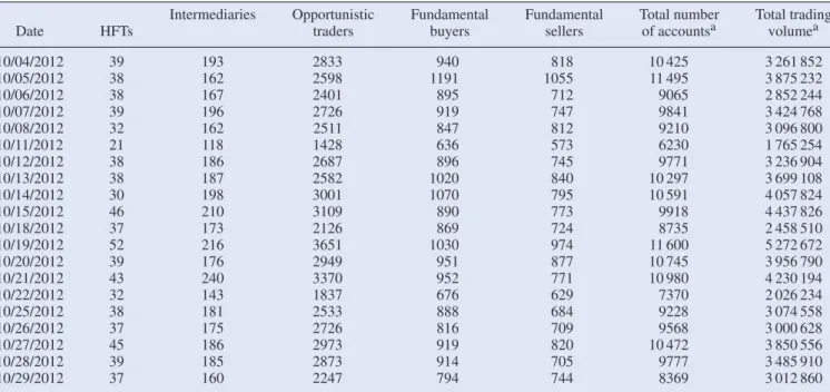
In consultation with the authors ofKirilenkoet al.(2011), we choose the standard deviation of an account’s net position measured on the event clock as a measure of an account’s holding fluctuation. With this definition, we find that a 1.5% fluctuation is too stringent for HFTs, because many high trading volume accounts are classified as opportunistic traders, while in reality their end of day positions are still very low compared with other opportunistic traders. Therefore, it is adequate to relax the first criterion requiring that the standard deviation of the account’s net holdings throughout the day is less than its end of day holding level. We find that the newly adjusted criteria classify most high volume trading accounts as HFTs, and this classification rule is validated from the registration informa-tion we can acquire. Without this adjustment, almost all the top trading accounts are incorrectly classified as opportunistic traders. Table1summarizes the results after applying the new classification rule demonstrating that the modified classifica-tion criteria identified more HFTs. On average, there are 38 HTF accounts, 181 intermediary accounts, 2658 opportunistic accounts, 906 fundamental buyer accounts, 775 fundamental seller accounts, and 5127 small trader accounts. Over the 4-week period, only 36% of the 120 accounts are consistently
Table 1. The E-Mini S&P 500 futures market data summary.
Intermediaries Opportunistic Fundamental Fundamental Total number Total trading
Date HFTs traders buyers sellers of accountsa volumea
10/04/2012 39 193 2833 940 818 10 425 3 261 852 10/05/2012 38 162 2598 1191 1055 11 495 3 875 232 10/06/2012 38 167 2401 895 712 9065 2 852 244 10/07/2012 39 196 2726 919 747 9841 3 424 768 10/08/2012 32 162 2511 847 812 9210 3 096 800 10/11/2012 21 118 1428 636 573 6230 1 765 254 10/12/2012 38 186 2687 896 745 9771 3 236 904 10/13/2012 38 187 2582 1020 840 10 297 3 699 108 10/14/2012 30 198 3001 1070 795 10 591 4 057 824 10/15/2012 46 210 3109 890 773 9918 4 437 826 10/18/2012 37 173 2126 869 724 8735 2 458 510 10/19/2012 52 216 3651 1030 974 11 600 5 272 672 10/20/2012 39 176 2949 951 877 10 745 3 956 790 10/21/2012 43 240 3370 952 771 10 980 4 230 194 10/22/2012 32 143 1837 676 629 7370 2 026 234 10/25/2012 38 181 2533 888 684 9228 3 074 558 10/26/2012 37 175 2726 816 709 9568 3 000 628 10/27/2012 45 186 2973 919 820 10 472 3 850 556 10/28/2012 39 185 2873 914 705 9777 3 485 910 10/29/2012 37 160 2247 794 744 8369 3 012 860
aThe remaining accounts consist of the small trader accounts.
classified as the same type of traders. If we rank these accounts by their daily trading volume, we find that only 40% of the top 10 accounts are consistently classified as the same trader types. The variation occurs among the HFTs, intermediaries and opportunistic traders.
3. Markov decision process model of market dynamics In this section, we develop a Markov decision process (MDP) model of trader behaviour. This model will then serve as the basis for the inverse reinforcement learning process described in section4.
3.1. MDP background and notation
The primary aim of our trading behaviour-based learning ap-proach is to uncover decision-makers’ policies and reward functions through the observations of an expert whose decision process is modelled as an MDP. In this paper, we restrict our attention to a finite countable MDP for easy exposition, but our approach can be extended to continuous problems if desired. A discounted finite MDP is defined as a tupleM = (S,A,P, γ,r), where
• S = {sn}nN=1is a set ofNstates. LetN = {1,2,· · · ,N}.
• A= {am}mM=1is a set ofMactions. LetM= {1,2, . . . ,M}. • P =Pam
M
m=1is a set of state transition probabilities (here
Pamis aN×Nmatrix where each row, denoted asPam(sn,: ), contains the transition probabilities upon taking action am in statesn. The entryPam(sn,sn)is the probability of moving to statesn,n∈N in the next stage.).
• γ ∈ [0,1]is a discount factor.
• rdenotes the reward function, mapping fromS×Ato
with the property that r(sn,am)
n∈N
Pam(sn,sn)r(sn,am,sn) wherer(sn,am,sn)denotes the function giving the reward of moving to the next statesn after taking actionam in current statesn. The reward functionr(sn,am)may be further reduced tor(sn), if we neglect the influence of the action. We user for reward vector through out this paper. If the reward only depends on state, we haver=(r(s1), . . . ,r(sN)). If we letr be the vector of the reward depending on both state and action. We have
r=(r1(s1), . . . , r1(sN), . . . ,rM(s1), . . . , rM(sN))
=( r1, . . . , rM).
In an MDP, the agent selects an action at each sequential stage, and we define apolicy (behaviour) as the way that the actions are selected by a decision-maker/agent. Hence, this process can be described as a mapping between state and ac-tion, i.e. a random state-action sequence s0,a0,s1,a1, . . .st, at,· · ·,†wherest+1is connected to(st,at)byP
at(st,st+1). We also define rational agents as those that behave according to the optimal decision rule where each action selected at any stage maximizes the value function. The value function for a policyπ evaluated at any state s0 is given as Vπ(s0) = E[∞t=0γtr(st,at)|π]. This expectation is over the distribu-tion of the state sequences0,s1, . . .given the policyπ =
μ0, μ1, . . ., whereat =μt(st),μt(st)∈U(st)andU(st)⊂ A. The objective at statesis to choose a policy that maximizes the value of Vπ(s). A policy π∗ is an optimal policy, if is
†Superscripts represent time indices. For examplestandat, with the
upper-indext∈ {1,2, . . .}, denote state and action at the t-th horizon
stage, whilesn(oram) represents the n-th state (or m-th action) inS
thenVπ∗(s0)=supπE[∞t=0γtr(st,at)|π]. Similarly, there is another function called the Q-function (or Q-factor) that judges how well an action is performed in a given state. The notationQπ(s,a)represents the expected return from states when actionais taken and thereafter policyπ is followed.
In the infinite-horizon case, the stationary Markovian struc-ture of the problem implies that the only variable that affects the agent’s decision rule and the corresponding value function should be time invariant. We then have the essential theory of MDPs (Bellman 1957) as follows:
Th e o r e m 3.1 (Bellman Equations) Given a stationary pol-icyπ,∀n∈N,m∈M, Vπ(sn)and Qπ(sn,am)satisfy
Vπ(sn)=r(sn, π(sn))+γ n∈N Pπ(sn)(sn,sn)Vπ(sn), Qπ(sn,am)=r(sn,am)+γ n∈N Pam(sn,sn)Vπ(sn).
Th e o r e m 3.2 (Bellman Optimality) π is optimal if and only if,∀n∈N,π(sn)∈arg maxa∈AQπ(sn,a).
Based on the above theorem of MDPs, we have the following equations to represent the Q-function as a the reward function.
Qπ(sn,am)=rm(sn)+γPam(sn,:)(I−γPπ)−1rm, wherePπ represents the state transition probability matrix for following policyπat every state, andrmrepresents the reward vector under actionam.
3.2. Constructing an MDP model from order book data
Figure1shows the entire life-cycle of an order initiated by a client of an exchange. The order book audit trail data contains these messages, and the entire order history (i.e. order creation, order modifications, fills, cancellation, etc.) can be retrieved and analyzed. To construct an MDP model of trader behaviour, we first reconstruct the limit order book using the audit trail messages. The order book then contains bid/ask prices, market depth, liquidity, etc. During this process on the E-Mini data described in section2.1, we processed billions of messages for each trading date, and built price queues using the price and time priority rule.
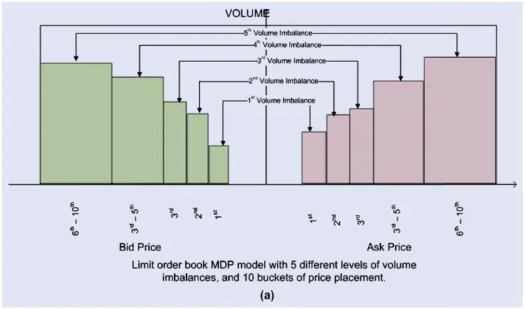
In this construction process, we choose event tick time rather than natural wall clock time. In other words, every activity including arrival of a new order, cancellation of an existing order, and placement of a market order is counted as one tick. Once we have the order book at any given event tick, we take the market depth at five different levels as our base variables and then discretize these variables to generate an MDP model state space. This study extends the MDP model documented byYanget al.(2012) to obtain five variables, i.e. order volume imbalance between the best bid and the best ask prices, order volume imbalance between the 2nd best bid and the 2nd best ask prices, order volume imbalance between the 3rd best bid and the 3rd best ask prices, the order book imbalance at the 5th best bid and the 5th ask prices, and the inventory level/holding position (see figure2(b)). Then we discretize the values of the five variables into three levels defined as high (above μ+ 1.96σ), neutral (μ±1.96) and low (belowμ−1.96σ). Based on our observation that the first three best bid and ask prices
change the most, we find that it is critical to include the first three-level order book imbalance variables in modelling the limit order book dynamics. As argued byYanget al.(2012), these volume-related variables reflect the market dynamics on which the traders/algorithms depend to place their orders at different prices.
As the volume imbalance at the best bid/ask prices is the most sensitive indicator of the trading behaviour of HFTs, intermediaries and some of the opportunistic traders, we also hypothesize that the volume imbalance at other prices close to the book prices will be useful in inferring trader behaviour.
As demonstrated in previous work (Yang et al. 2012), the
private variable of a trader’s inventory level provides crit-ical information about trader’s behaviour. Traders in high-frequency environments strive to control their inventory levels as a critical measure of controlling the risk of their position (Easley et al.2010, Brogaard 2010, Kirilenko et al. 2011). HFTs and Market-makers tend to turn over their inventory level five or more times a day and to hold very small or even zero inventory positions at the end of the trading session. These observations provide strong support for the introduction of a position variable to characterize trader behaviour in our model. Therefore, together with the volume imbalance variables, we propose a computational model with 35=243 states.
Next, we need to define the action space. In general, there are three types of actions: placing a new order, cancelling an existing order, or placing a market order. We divide the limit order book into 10 buckets at any given point of time by the following price markers: the best bid price, the 2nd best bid price, the 3rd best bid price, between the 4th and 5th bid prices, below the 5th best bid price, the best ask price, the 2nd best ask price, the 3rd best ask price, between the 4th and 5th ask prices, and above the 5th best ask price. Then, at any given point of time, a trader can take 22 actions. The price markers used to define the price ranges are illustrated in figure2. We define the order volume imbalance through buckets. In other words, the boundaries of these buckets define the volume between the two adjacent best price levels. In case of missing prices between the two adjacent best price levels, we only count the total volume between them. Therefore, missing prices between these best price levels will be acceptable for our volume imbalance modelling. We use unit size for all the actions. Orders other than unit size are treated as repeated actions without state transition. Once we have both the state space and the action space defined, we can then construct an MDP model where traders interact with the order book. All actions from a trader can be correlated with certain states in a probabilistic sense. From trading strategy perspective, traders may choose to either react to or influence order book movements. Although in most of the cases, traders may choose to react to market changes to achieve their investment objectives, anticipative or aggressive strate-gies are also widely used. To some degree, certain aggressive strategies through which specific actions are designed to create desirable market conditions for themselves can be defined as manipulative, but it is out of the scope of this paper. Over all, a predefined trading strategy would consistently take certain actions under certain market conditions within its permissible or desirable inventory levels until these conditions change. This process can be captured in a transition matrix of an MDP model. Essentially, we have a 243x243 matrix for each action, which
Figure 1. CME globex order lifecycle.T1: Trader submits a new order; T2: The state of an order is changed, if a stop is activated; T3: A trader may choose to cancel an order, and the state of an order can be modified multiple times; T4: When an order is partially filled, the quantity remaining decreases; T5: Order elimination is similar to order cancellation except it is initiated by the trading engine; T7: An order may be filled completely; T6: Trades can be eliminated after the fact by the exchanges.
Figure 2. Order book MDP model:This graph shows the state variables used in the MDP model.
describes the Markovian decision process of a trading strategy. In reality, these transition matrices are very sparse. For each action, there are only a few desirable states, and most of the
elements are zeros. In the end, it is those scarce transitions that reflect the uniqueness of the corresponding strategies. In addition, we define a non-action in which the traders choose
to do nothing as the market moves. Eventually, we have a 23x243x243 3-dimensional matrix for each trader based on the frequencies we calculated from the sample data.
4. Inverse reinforcement learning
Given an MDPM=(S,A,P, γ,r), let us define the inverse Markov decision process (IMDP)MI=(S,A,P, γ,O). The processMI includes the states, actions and dynamics ofM, but lacks a specification of the reward function,r. By way of compensation,MIincludes a set of observationsOthat consists of state-action pairs generated through the observation of a decision-maker. We can define theinverse reinforcement
learn-ing (IRL) problem associated with MI = (S,A,P, γ,O)
to be that of finding a reward function such that the observations
O could have come from an optimal policy for
M=(S,A,P, γ,r). The IRL problem is, in general, highly under-specified, which has led researchers to consider various models for restricting the set of reward functions under con-sideration.Ng and Russel(2000), in a seminal consideration of IMDPs and associated IRL problems, observed that, by the optimality equations, the only reward vectors consistent with an optimal policyπare those that satisfy the set of inequalities (Pπ−Pa)(I−γPπ)−1r≥0, ∀a∈A, (1) where Pπ is the transition probability matrix relating to ob-served policyπandPadenotes the transition probability ma-trix for other actions. Note that the trivial solutionr=0 sat-isfies the constraints (1), which highlights the under-specified nature of the problem and the need for reward selection mech-anisms.
In the machine learning and artificial intelligence literature, a principal motivation for considering IRL problems is the idea of apprenticeship learning, in which observations of state-action pairs are used to learn the policies followed by experts for the purpose of mimicking or cloning behaviour. By its na-ture, apprenticeship learning problems arise in situations where it is not possible or desirable to observe all state-action pairs for the decision-maker’s policy. The basic idea of apprenticeship learning through IRL is to first use IRL techniques to learn the reward function (vector) and then use that function to define an MDP problem, which can then be solved for an optimal policy. Our process is quite different. We learn the reward function with IRL and then directly use the rewards as features for classifying and clustering traders or trading algorithms.
4.1. Linear IRL
Ng and Russel(2000) advance the idea choosing the reward function to maximize the difference between the optimal and suboptimal policies, which can be done using a linear program-ming formulation.
Most of the existing IRL algorithms make some assumption about the form of the reward function. Prominent examples include the model inNg and Russel (2000), which we term linear IRL (LIRL) because of its linear nature. In LIRL, the reward function is written linearly in terms of basis functions,
and effort is made to maximize the quantity
s∈S
[Qπ(s,a)− max a∈A\aQ
π(s,a)], ∀a∈A. (2) The optimization problem inNg and Russel(2000) is equiva-lent to the following optimization program:
maxr s∈Sβ(s)−λ s∈S|r(s)| s.t. (Pπ−Pa)(I−γPπ)−1r ≥β(s), ∀a∈A,∀s∈S β(s) ≥0, ∀s∈S,
whereλ is a regularization parameter included to encourage sparse solution vectors, andβ(s)is the lower bound of the function:Qπ(s,a)−maxa∈A\a Qπ(s,a).Yanget al.(2012) use this approach to find a feature space that can be used to classify and cluster simulated trading agents. Here, reward is defined as a function of state only, which means that agents do not distinguish actions in seeking rewards under certain conditions. This action-independent approximation for reward is discussed further in the context of the Bayesian IRL frame-work.
4.2. Bayesian IRL framework
Ramachandran andAmir(2007) originally proposed a Bayesian Framework for IRL. The posterior over reward is written as:
p(r|O)= p(O|r)p(r)∝
(s,a)∈O
p(a|s,r).
Then, the IRL problem is written as maxrlogp(O|r)+logp(r). For many problems, however, the computation ofp(r|O)may be complicated and some algorithms use Markov chain Monte Carlo (MCMC) to sample the posterior probability. Below, we adopt a different approach that uses the idea of selecting reward on the basis ofmaximum a posteriori(MAP) estimate computed using convex optimization.
4.3. Gaussian process IRL
We now turn to an IRL problem that addresses observations from a decision-making process in which the reward function has been contaminated by Gaussian noise. In particular, we assume that the reward vector can be modelled asr+N(0, σ2), where N(0, σ2) is Gaussian noise. In the financial trading problem setting, we may observe certain trading behaviour over a period of time, but we may not observe the complete polices behind a particular trading strategy. As discussed ear-lier, different trading strategies tend to look at different time horizons. Therefore, the observation period becomes critical to the learning process. Furthermore, two types of errors may be introduced into our observations: the first type of error may be introduced during our modelling process. Resolution of these discrete models will introduce errors into our observations. The second potential source of error is the strategy execution process. Execution errors will occur due to the uncertainty of market movements and will eventually appear in our observa-tions, confounding our efforts to determine the true policy. Overall, there are two types of challenges in this learning problem: the uncertainty about reward functions given the
observation of decision behaviour and the ambiguity involved in observing multiple actions at a single state.
Qiao and Beling(2011) argue for two different modelling techniques in learning reward functions. To lessen the ambi-guity of observing multiple actions at a state, they argue that Bayesian inference should be the basis for understanding the agent’s preferences over the action space. This argument is reasonable because the goal of IRL is to learn the reward sub-jectively perceived by the decision-maker from whom we have collected the observation data. The intuition is that decision-makers will select some actions at a given state because they prefer these actions to others. These preferences are among the countable actions that can be used to represent multiple observations at one state.
Here, we use two examples to demonstrate how the ac-tion preference relaac-tionships have been constructed based on
the MDP model and observed actions. Table 2 shows two
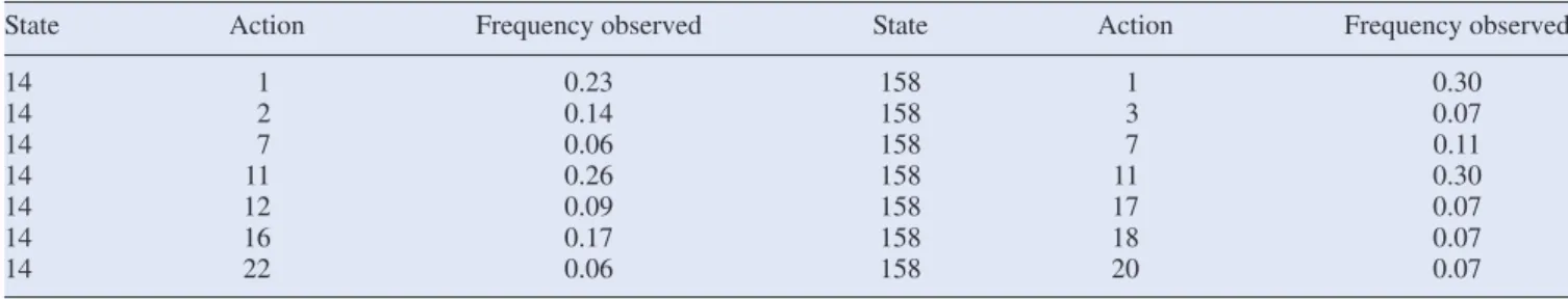
example states with multiple observed actions. We then sort the frequency in descending order and construct a two-layer graph: the top layer has the most frequently observed actions and the bottom layer holds all the other actions. Based on this preference observation, we can construct two preference graphs as shown in figure3. The state transition matrix can be constructed for the entire market for the observation period. In our MDP model, we have a 243×243 matrix for every single action.
In the following, we first introduce the preference theory for the IMDP model, and then we formalize the idea of modelling the reward function as a Gaussian process under the Bayesian inference framework.
4.3.1. Action preference learning. In this section, we first define the action preference relationship and the action pref-erence graph. At state sn, ∀ˆa,aˇ ∈ A, we define the action preference relationas:
(i) Actionaˆ is weakly preferred toaˇ, denoted asaˆ sn aˇ, ifQ(sn,aˆ)≥ Q(sn,aˇ);
(ii) Actionaˆis strictly preferred toaˇ, denoted asaˆsn aˇ, if Q(sn,aˆ) >Q(sn,aˇ);
(iii) Actionaˆ is equivalent toaˇ, denoted asaˆ ∼sn aˇ, if and only ifaˆ sn aˇandaˇsn aˆ.
Anaction preference graphis a simple-directed graph show-ing preference relations among the countable actions at a given state. At statesn, the action preference graphGn =(Vn,En) comprises a setVn of nodes together with a setEn of edges. For the nodes and edges in graphGn, let us define
(i) Each node represents an action inA. Define a one-to-one
mappingϕ :Vn→A.
(ii) Each edge indicates a preference relation.
Furthermore, we make the following assumption as a rule to build the preference graph, and then we show how to draw a preference graph at statesn:
At statesn, if actionaˆ is observed, we have the following preference relations:aˆsn aˇ,∀ˇa ∈A\
ˆ
a.
It is, therefore, straightforward to show the following ac-cording to Bellman optimality. The variableaˆ is observed if
and only ifaˆ ∈arg maxa∈AQ(sn,a). Therefore, we have Q(sn,aˆ) > Q(sn,aˇ), ∀ˇa∈A\aˆ
According to the definition on preference relations, it follows that if Q(sn,aˆ) > Q(sn,aˇ), we haveaˆ sn aˇ. Hence, we can show that the preference relationship has the following properties:
(1) Ifaˆ,aˇ ∈A, then at statesneitheraˆ sn aˇoraˇ sn aˆ. (2) Ifaˆ sn aˇandaˇ sn a˜, thenaˆsn a˜.
At this point, we have a simple representation of the action preference graph that is constructed by a two-layer directed graph. We may have either multiple actions atsnas in figure 4(a) or a unique action atsnas in figure4(b). In this two-layer directed graph, the top layerVn+is a set of nodes representing the observed actions and the bottom layer Vn− contains the nodes denoting the other actions. The edge in the edge set Encan be represented by a formulation of its beginning node u and ending nodev. We write the k-th edge as(u → v)k if u∈Vn+, v∈Vn−, or the l-th edge(u↔v)lifu ∈Vn−, v∈Vn−. Recall the mapping betweenVnandA, the representationu→ vindicates that actionϕ(u)is preferred overϕ(v). Similarly, u↔vmeans that actionϕ(u)is equivalent toϕ(v).
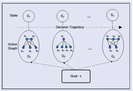
In the context of financial trading decision process, we may observe multiple actions from one particular trader under cer-tain market conditions. That is to say that the observation data Omay represent multiple decision trajectories generated by non-deterministic policies. To address IRL problems in those cases,Qiao and Beling(2011) propose to processOinto the form of pairs of state and preference graphs similar to the representation shown in figure5, and then we apply Bayesian inference using the new formulation.
According toQiao and Beling(2011), we can representO as shown in figure5. At statesn, its action preference graph is constructed by a two-layer directed graph: a set of nodesVn+in the top layer and a set of nodesVn−in the bottom layer. Under the non-deterministic policy assumption, we adopt a reward structure depending on both state and action.
4.3.2. Gaussian reward process. Recall that the reward de-pends on both state and action, and considerrm, the reward related to action am, as a Gaussian process. We denote by km(si,sj) the function generating the value of entry (i,j) for covariance matrixKm, which leads torm ∼ N(0,Km). Then the joint prior probability of the reward is a product of multivariate Gaussian, namely p(r|S) = mM=1p(rm|S) andr ∼ N(0,K). Note thatris completely specified by the positive definite covariance matrixK, which is block diagonal in the covariance matrices{K1,K2. . . ,KM}based on the as-sumption that the reward latent processes are uncorrelated . In practice, we use a squared exponential kernel function, written as:
km(si,sj)=e
1
2(si−sj)Tm(si−sj)+σ2
mδ(si,sj),
where Tm = κmIandI is an identity matrix. The function δ(si,sj)=1, whensi =sj; otherwiseδ(si,sj)=0. Heresi andsj are feature vectors. If the feature dimension is 5 or in R5, the difference between two vectors is a 5-dimension vector. Under this definition the covariance is almost unity between
Figure 3 . Action p re fer ence g raph examples: (a). This graph shows an example action p reference g raph at state 158. (b). This graph shows an example action p reference g raph at state 14.
Table 2. Action preference graph examples.
State Action Frequency observed State Action Frequency observed
14 1 0.23 158 1 0.30 14 2 0.14 158 3 0.07 14 7 0.06 158 7 0.11 14 11 0.26 158 11 0.30 14 12 0.09 158 17 0.07 14 16 0.17 158 18 0.07 14 22 0.06 158 20 0.07
Figure 4. Examples preference graphs:(a) An example of observing two actions at a state. (b) An example of a unique observation at a state.
variables whose inputs are very close in the Euclidean space, and decreases as their distance increases.
Then, the GPIRL algorithm estimates the reward function by iteratively conducting the following two main steps:
(1) Get estimation of rM A P by maximizing the posterior p(r|O), which is equal to minimize −logp(O|r)− logp(r|θθθ), where θθθ denotes the vector of
hyper-parameters including κm and σm that control the
Gaussian process.
(2) Optimize the hyper-parameters by using gradient decent method to maximize logp(O|θθθ,rM A P), which is the Laplace approximation of p(θθθ|O).
4.3.3. Likelihood function and MAP optimization. GPIRL adopts the following likelihood functions to capture the strict preference and equivalent preference, respectively.
p((aˆ sn aˇ)k|r)= Q(sn,aˆ)−Q(sn,aˇ) √ 2σ (3) p((aˆ ∼sn aˆ)l|r)∝e− 1 2(Q(sn,aˆ)−Q(sn,aˆ))2 (4) In equation (3), the function(x)=−∞x N(v|0,1)dv, where N(v|0,1)denotes a standard Gaussian variable.
As we stated earlier, if we model the reward functions as being contaminated with Gaussian noise that has a mean of zero and an unknown varianceσ2, we can then define the likelihood function for both the k-th strict preference relation and the l-th equivalent preference relation. Finally, we can formulate the following proposition:
Pr o p o s it io n 4.1 The likelihood function, given the evidence of the observed data (Oin the form of pairs of state and action
preference graph (G), is calculated by p(O|r)∝ p(G|S,r)= N n=1 p(Gn|sn,r) = N n=1 nn k=1 p((aˆ sn aˇ)k|r) mn l=1 p((aˆ∼sn aˆ)l|r), (5) where nn denotes the number of edges for strict preference andmnmeans the number of edges for equivalent preference at statesn.
In conclusion, the probabilistic IRL model is controlled by
the kernel parametersκm andσm which compute the
covari-ance matrix of reward realizations, and byσ which tunes the noise level in the likelihood function. We put these parameters into the hyper-parameter vectorθθθ =(κm, σm, σ ). More often than not, we do not have prior knowledge about the hyper-parameters. And then we can apply maximum a posterior esti-mate to evaluate the hyper-parameters.
Essentially, we now have a hierarchical model. At the lowest level, we have reward function values encoded as a parameter vector r. At the top level, we have hyper-parameters in θθθ controlling the distribution of the parameters. Inference takes place one level at a time. At the bottom level, the posterior over function values is given by Bayes’ rule:
p(r|S,G,θθθ)= p(G|S,θθθ,r)p(r|S,θθθ)
p(G|S,θθθ) . (6) The posterior combines the prior information with the data, reflecting the updated belief aboutrafter observing the deci-sion behaviour. We can calculate the denominator in equation (6) by integrating p(G|S,θθθ,r)over the function space with respect tor, which requires a high computational capacity. For-tunately, we are able to maximize the non-normalized posterior density ofrwithout calculating the normalizing denominator, as the denominatorp(G|S,θθθ)is independent of the values ofr.
Figure 5. Observation structure for MDP.
In practice, we obtain the maximum posterior by minimizing the negative log posterior, which is written as
U(r) 1 2 M m=1 rmTK−m1rm− N n=1 nn k=1 ln Q(sn,aˆ)−Q(sn,aˇ) √ 2σ + N n=1 mn l=1 1 2(Q(sn,aˆ)−Q(sn,aˆ ))2 (7)
Qiao and Beling(2011) present a proof that Proposition (7) is a convex optimization problem. At the minimum ofU(r)we have
∂U(r) ∂rm =
0⇒ ˆrm=Km(∇logP(G|S,θθθ,rˆ)) (8) whererˆ =(rˆ1, . . . ,rˆam, . . . ,rˆm). In equation (8), we can use Newton’s method to find the maximum ofUwith the iteration,
ˆ rnewm = ˆrm− ∂2U(r) ∂rm∂rm −1 ∂U(r) ∂rm
5. Experiment with the E-Mini S&P 500 equity index futures market
In this section, we conduct two experiments using the MDP model defined earlier to identify algorithmic trading strate-gies. We consider the six trader classes defined byKirilenko et al.(2011), namely high-frequency traders, market-makers, opportunistic traders, fundamental buyers, fundamental sellers and small traders. As we argue earlier, the focus of our study will be more on HFTs and market-makers due to the large daily volume and their potential impact to the financial markets. In Kirilenkoet al.(2011)’s paper, there are only about from 16 to 20 HFTs on the S&P500 Emini market. Although this is a small population, their impact to the market has drawn increased attention from policy-makers, regulators and academia. That is why we focus our attention on this small population. Among the roughly 10 000 trading accounts for the S&P500 Emini
market, we narrow down to about 120 accounts based their high daily trading volume. In the first experiment, we select the top 10 trading accounts by their volume and end-of-the-day positions. In this we guarantee our subjects are HTFs. In the second experiment, we randomly select 10 out of the 120 accounts. This selection criterion ensures that our subjects are of either HTF or market-making strategies. With these two experimentations we show the performance of our IRL-based approach to identify the high impact population of the algorithmic trading strategies.
5.1. Trader behaviour identification
Yanget al.(2012) examine different trading behaviours using a linear IRL (LNIRL) algorithm with the simulated E-Mini S&P 500 market data. That MDP model contains three variables: the volume imbalance at the bid/ask prices, the volume imbalance at the 3rd best bid/ask prices and the position level. Although this MDP model is relatively simple, it is evident from the experimental results that the IRL reward space is effective in identifying trading strategies with a relatively high accuracy rate.
This paper tries to address two important issues during the modelling process to solve a realistic market strategy learning problem using real market data. The first issue is that in reality, we often do not have a complete set of observations of a trader’s policies. As the market presents itself as a random process in terms of both prices and volume, it is unlikely that we will be able to capture all possible states during our observation window. In contrast, the study performed byYanget al.(2012) assumes complete observation of a trader’s decision policies for the simulated trading strategies. In other words, the policies simulated by a distribution can be completely captured when the simulation is run long enough. The convergence of these simulated policies and the testing results are consistent with their assumptions. However, when we use real market data to
![Table 3. Pair-wise trader classification using SVM binary classification using LNIRL. [,1] [,2] [,3] [,4] [,5] [,6] [,7] [,8] [,9] [,10] [1,] 0 .0000 0 .5437 0 .5187 0 .4812 0 .6375 0 .4812 0 .5312 0 .5750 0 .7750 0 .5937 [2,] 0 .5437 0 .0000 0 .5250 0 .51](https://thumb-us.123doks.com/thumbv2/123dok_us/1279281.2671940/16.892.83.832.128.316/table-pair-trader-classification-using-binary-classification-lnirl.webp)


