Ministry of Higher Education and Scienti…c Research MOHAMED KHIDER UNIVERSITY, BISKRA FACULTY of EXACT SCIENCES, SIENCE of NATURE and LIFE
DEPARTMENT of MATHEMATICS
A thesis presented for the degree of :
Doctor in Mathematics In the Filled of : Statistics
By
Madiha TOUR Title :
On improve boundary e¤ect in kernel distribution
estimation
Members of the jury :
BRAHIM BRAHIMI Prof. University of Biskra Chairman Abdallah SAYAH M.C.A. University of Biskra Supervisor Halim ZEGHDOUDI M.C.A University of Annaba Examinator Djabrane YAHIA M.C.A University of Biskra Examinator Fatah BENATIA M.C.A University of Biskra Examinator
Ministère de l’Enseignement Supérieur et de la Recherche Scienti…que
UNIVERSITÉ MOHAMED KHIDER, BISKRA
FACULTÉ des SCIENCES EXACTES et des SCIENCES de la NATURE et de la VIE DÉPARTEMENT DE MATHÉMATIQUES
Thèse présentée en vue de l’obtention du Diplôme : Doctorat en Mathématiques
Option: Statistique Par
Madiha TOUR Title :
Sur l’Amélioration d’e¤et du bord dans estimation à
noyau de la distribution
Membres du Comité d’Examen :
Brahim BRAHIMI Prof. Université de Biskra Président Abdallah SAYAH M.C.A. Université de Biskra Encadreur Halim ZEGHDOUDI M.C.A Université d’Annaba Examinateur Djabrane YAHIA M.C.A Université de Biskra Examinateur Fatah BENATIA M.C.A Université de Biskra Examinateur
Je dédie ce travail
Mes chers père et mère, Pour tous les sacri…ces qu’ils ont consentis pour me permettre de pour suivre mes études dans les meilleures conditions possibles et pour n’avoir jamais cessé de m’encourager tout au long de mes années d’étude.
Ames très chers frères et sœurs. Atoute ma famille.
Mes premiers remerciements vont tout naturellement à Dieu le tout puissant pour la volonté, la santé et la patience qu’il m’a donnée pour réaliser mon travail de recherche.
Je tiens à exprimer ma profonde gratitude, mes sincères et chaleureux remerciements à mon directeur de thèse, Monsieur le Dr. Sayah Abdallah, pour la con…ance qu’il m’a accordée en acceptant d’encadrer ce travail doctoral, par ses multiples conseils. J’ai été extrêmement sensible à ses qualités humaines d’écoute et de compréhension durant toutes les étapes de cette recherche.
Je remercie vivement Monsieur le Professeur Brahimi Brahim qui m’a fait le grand honneur de présider le jury. Mes remerciements vont aussi aux membres du jury, le Dr. Zeghdoudi Halim, le Dr. Yahia Djabrane et le Dr. Benatia Fatah pour avoir accepté d’examiner et bien évaluer ma thèse. Merci pour vos corrections et remarques constructives.
Je remercie chaleureusement tous les membres du Laboratoire de Mathématiques Ap-pliquées et surtout le Professeur Meraghni Djamel de son aide.
Je tiens à remercier ma famille pour leurs encouragements, soutien et sacri…ce apportés tout au long de mon cheminement scolaire et universitaire. Merci à toute personne ayant contribué directement ou indirectement à ce travail.
In this thesis, we propose a new estimator for improve boundary e¤ects in kernel estimator of the heavy-tailed distribution function specially the Pareto-type distributions and its bias, variance and mean squared error are determined. Kernel methods are widely used in many research areas in statistics. However, kernel estimators su¤er from boundary e¤ects when the support of the function to be estimated has …nite end points. Boundary e¤ects seriously a¤ect the overall performance of the estimator. To remove the boundary e¤ects, a variety of methods have been developed in the literature, the most widely used is the re‡ection, the transformation ... In this thesis, we introduce a new method of boundary correction when estimating the heavy-tailed distribution function. Our technique is kind of a generalized re‡ection method involving re‡ecting a transformation of the observed data by modi…ed Champernowne distribution function.
Dans cette thèse, nous proposons un nouveau estimateur pour améliorer les e¤ets de bord dans l’estimateur à noyau de la fonction de distribution à queue lourde spécialement les distributions de type Pareto, son biais, variance et l’erreur quadratique moyenne de cette estimateur sont déterminées. Les méthodes du noyau sont largement utilisées dans de nombreux domaines de recherche en statistiques. Cependant, les estimateurs à noyau sou¤rent des problèmes d’e¤ets aux bords de leur support. Les e¤ets de bord a¤ectent sérieusement la performance globale de l’estimateur. Pour corrigé ces e¤ets de bord, une variété de méthodes ont été développées dans la littérature, la plus utilisée est la ré‡exion, la transformation ... Dans cette thèse, nous introduisons une nouvelle méthode de correc-tion de l’e¤et de bord lors de l’estimacorrec-tion de la fonccorrec-tion de distribucorrec-tion à queue lourde. Notre technique est en quelque sorte une méthode de ré‡exion généralisée impliquant une transformation des données observées par une fonction de distribution de Champernowne modi…ée.
Dédicace i
Remerciements ii
Abstract iii
Résumé iv
Table of Contents v
Liste des …gures vii
Liste des tableaux viii
Introduction 1
1 Nonparametric distribution estimation 6
1.1 Empirical distribution function . . . 7
1.1.1 Properties of EDF . . . 7
1.2 Kernel method . . . 9
1.2.1 Kernel distribution function estimator . . . 11
2 Heavy-tailed distribution 18 2.1 Heavy-tailed distribution . . . 19
2.1.1 Examples of heavy-tailed distributions . . . 21
2.2 Classes of heavy-tailed distributions . . . 22
2.2.1 Regularity varying distribution functions . . . 23
2.2.2 Subexponential distribution functions . . . 25
3 Transformation in kernel density estimation for heavy-tailed distribu-tions 29 3.1 Kernel density estimator and boundary e¤ects . . . 30
3.2 Methods for removing boundary e¤ects . . . 32
3.3 Champernowne distribution . . . 35
3.3.1 Modi…ed Champernowne distribution . . . 36
3.4 Density estimation using Champernowne transformation . . . 39
3.4.1 Asymptotic theory for the transformation kernel density estimator . 42 4 A modi…ed Champernowne transformation to improve boundary e¤ect in kernel distribution estimation 46 4.1 Introduction . . . 47
4.2 Boundary kernel distribution estimator . . . 49
4.3 The proposed estimator . . . 52
4.4 Simulation Studies . . . 55
4.5 Proofs . . . 57
Conclusion 66
Bibliographie 66
1.1 Rate of kernels : Gaussian, Epanechnikov, Biweight and Triweight . . . 11
3.1 Boundary e¤ect in kernel density estimation . . . 32 3.2 Modi…ed Champernowne distribution function, (M = 3; = 0:5) . c = 0
dashed line and c= 2 solid line. . . 38 3.3 Modi…ed Champernowne distribution function, (M = 3; = 2) . c = 0
dashed line and c= 2 solid line. . . 39 3.4 Usual kernel estimator and Champernowne transformation estimator. . . . 45
1.1 Some kernel functions. I(.) denotes the indicator function. . . 11
2.1 Regularly varying distribution functions . . . 25
2.2 Subexponential distribution . . . 28
4.1 Distributions used in the simulation studies. . . 55
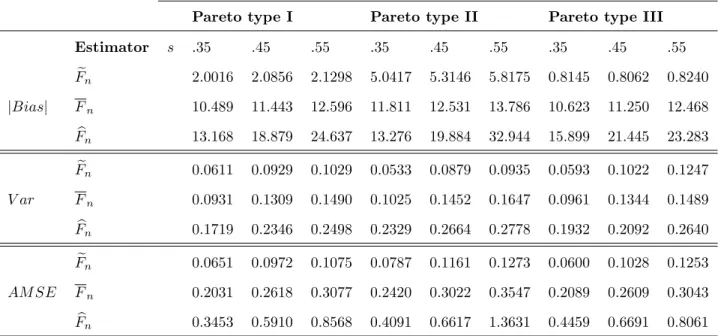
4.2 Bias, Var and AMSE Values Over the Boundary Region for sample size n=50. Results are re-scaled by the factor 0.001. . . 64
4.3 Bias, Var and AMSE Values Over the Boundary Region for sample size n=200. Results are re-scaled by the factor 0.001. . . 64
4.4 Bais, Var and AMSE Values Over the Boundary Region for sample size n=400. Results are re-scaled by the factor 0.001. . . 65
4.5 AIMSE Values Over the Boundary Region. Results are re-scaled by the factor 0.001. . . 65
I
n the area of statistic, estimation of the unknown distribution function F(x); of a population is important. Other statistical methods that are dependent on knowledge of the distribution function include hypothesis testing and con…dence interval estimation. Existing methods to estimate on unknown distribution function from data can be classi…ed into two groups, namely : parametric and nonparametric methods. Parametric methods are dependent on assumption that the functional form of the distribution function is speci…ed. If it is known that the data are normally distributed with unknown mean and variance, the unknown parameters can be estimated from the data and the distribution function is then completely determined. If the assumption of normality cannot be made, then the parametric method of estimation cannot be used and a nonparametric method of estimation must be implemented. Here we consider only nonparametric estimators.Nonparametric kernel smoothing belongs to a general category of techniques for non-parametric estimations including : density, distribution, regression, quantiles, ... These estimators are now popular and in wide use with great success in statistical applications. Early results on kernel density estimation are due to Rosenblatt (1956) [51] and Parzen (1962) [47]. Good references in this area are Silverman (1986) [55], and Wand and Jones (1995) [61], and the form kernel regression estimator has been proposed by Nadaraya (1964) [46] and Watson(1964) [63]. While results in a kernel distribution estimator is in-troduced by authors such as Nadaraya(1964) [45] or Watson and Leadbetter(1964) [62]. Such an estimator arises as an integral of the Parzen-Rosenblatt kernel density estimator.
Kernel estimates may su¤er from boundary e¤ects. This type of boundary e¤ect for ker-nel estimators of curves with compact supports is well-known in regression and density function estimation frameworks. In the density estimation context, a various boundary bias correction methods have been proposed. Schuster (1999) [54] and Cline and Hart (1991) [14]considered the re‡ection method, which is most suitable for densities with zero derivatives near the boundaries. Boundary kernel method and local polynomial method are more general without restrictions on the shape of densities. Local polynomial method can be seen as a special case of boundary kernel method and draws much attention due to its good theoretical properties. Though early versions of these methods might produce negative estimates or in‡ate variance near the boundaries, remedies and re…nements have been proposed, see Müller (1991) [43], Jones (1993) [31], Jones and Foster (1996) [32], Cheng (1997) [11], Zhang and Karunamuni (1998; 2000) [67];[69] and Karunamuni and Alberts(2005) [34]. Cowling and Hall (1996) [15]proposed a pseudo-data method that es-timates density functions based on the original data plus pseudo-data generated by linear interpolation of order statistics. Zhang et al. (1999) [68]combined the pseudo-data, trans-formation and re‡ection methods. In the regression function estimation context, Gasser and Müller(1979) [25] identi…ed the unsatisfactory behavior of the Nadaraya Watson re-gression estimator for points in the boundary region. They proposed optimal boundary kernels but did not give any formulas. However, Gasser and Müller(1979) [25]and Müller (1988) [44]suggested multiplying the truncated kernel at the boundary zone or region by a linear function. Rice(1984) [50] proposed another approach using a generalized jackknife. Schuster(1985) [53]introduced a re‡ection technique for density estimation. Eubank and Speckman(1991) [20] presented a method for removing boundary e¤ects using a bias re-duction theorem. Kheireddine et al. (2015) [36] produce a General method of boundary correction in kernel regression estimation, we combine the transformation and re‡ection boundary correction methods.
other words, these e¤ects seriously a¤ect the performance of these estimators and these require good precision. A similar correction used in density estimation would be made for improve the theoretical performance of the usual kernel distribution function estimator at the boundary points. In this thesis we develop a new kernel estimator of the distribution function for heavy-tailed distributions based on the modi…ed Champernowne transforma-tion. We will concentrate not to estimate the distribution of X based on the samples
X1; :::; Xn but to estimate the distribution of Y based on the samples Y1; :::; Yn where
Yi =T(Xi).
Buch-Larsen et al. (2005) [7] suggested to choose T so that T(X) is close to the uniform distribution. They proposed a kernel estimator of the density of heavy-tailed distributions based on a transformation of set of the original data with a modi…ed Champernowne distribution that is a heavy-tailed Pareto-type, see Champernowne(1936; 1952) [8];[10], and applied to transformed data. The kernel estimator for heavy-tailed distributions has been studied by several authors Bolancé et al. (2003) [6], Clements et al. (2003) [13] and Buch-Larsen et al. (2005) [7]propose di¤erent families of parametric transformation that they all make the transformed distribution more symmetric than the original, which in many applications are generally highly asymmetric right. Sayah et al. (2010) [52] produce a kernel quantile estimator for heavy-tailed distributions using a modi…cation of the Champernowne distribution.
Our thesis is organized in4 chapters.
Chapter1;is an introduction to the nonparametric estimation of the distribution func-tion, a common problem in statistics is that of estimating a density f or a distribution function F from a sample of real random variables X1; :::; Xn independent and with the
same unknown distribution. The functionsf and F, as the characteristic function, com-pletely describe the probability distribution of the observations and to know a convenient
estimation can solve many statistical problems. The traditional estimator of the distrib-ution functionF is the empirical distribution function which is de…ned by
Fn(x) = 1 n n X i=1 I(Xi x):
This estimator is an unbiased estimator and consist of F(x). Another estimator of F is the kernel estimator Fbn which is de…ned by
b Fn(x) = 1 n n X i=1 K x Xi b ;
where K(x) = Rx1k(t)dt and k is a kernel function and b is the smoothing parameter. The asymptotic properties of Fbn was initiated by Nadaraya (1964) [45] and continued in
a series of papers among which we mention Winter(1973; 1979) [64];[65], Yamato (1973) [66], Reiss (1981) [49]:
Chapter 2, we focused on the presentation of the concept of heavy-tailed distributions and di¤erent classes of this type of distributions, an important classes of heavy-tailed distributions are that subexponential distribution and the regularity varying distribution with index > 0. A distribution has a heavy tailed if and only if its kurtosis is higher than the normal distribution that is equal to 3. There are others de…nitions so that a distribution is heavy-tailed that is the distributions which the exponential moment is in…nite.
Chapter 3; describes the transformation in kernel density estimation. Let X1; :::; Xn
a random sample of independent and identically distributed observations of a random variable with density function f; then the kernel density estimator at point x is
^ fn(x) = 1 nb n X i=1 k x Xi b ;
where b is the bandwidth or smoothing parameter, and k is the kernel function, usually it is a symmetric density function bounded and centred at zero. Silverman (1986) [55] or Wand and Jones(1995) [61] provide an extensive review of classical kernel estimation. For heavy-tailed distributions, the kernel density estimation has been studied by several authors : Buch-Larsen et al. (2005) [7], Clements et al. (2003) [13] and Bolancé et al. (2003) [6]. They have all proposed estimators based on a transformation of the original variable. The transformation method proposed initially by Wand et al. (1991) is very suitable for asymmetrical variables, it was based on the shifted power transformation family. Some alternative transformations such as the one based on a generalization of the Champernowne distribution it is preferable to other transformation density estimation approaches for distributions that are Pareto-like in the tail.
Chapter 4, in this chapter we present our result which is the estimation of heavy-tailed distributions based on a re‡ection method involving re‡ecting a transformation and using the modi…ed Champernowne transformation which is introduced in the work of Buch-Larcen et al. (2005) [7] in the case of density estimation for heavy-tails distributions, the new approach based on the modi…ed Champernowne distribution is the preferable method, because it has a good performance in most of the investigated situations.
Nonparametric distribution
estimation
N
onparametric methods are becoming increasingly popular in statistical analysis of economic problems. In most cases, this is caused by the lack of information, especially historical data, about the economic variable being analysed. Smoothing meth-ods concerning functions, such as density or distribution function, play a special role in a nonparametric analysis of economic phenomena. Knowledge of density function or distri-bution function, or their estimates, allows one to characterize the random variable more completely. It is true that one can often switch from an estimator of f to an estimator of F by integration and an estimator of F to an estimator of f by derivation. However one feature is noteworthy : it is the existence the empirical distribution functionFn.Es-timation of functional characteristics of random variables can be carried out using kernel methods. Nonparametric kernel distribution estimation is now popular and in wide use with great success in statistical applications.
1.1
Empirical distribution function
The best known and simplest nonparametric estimator of distribution function is the empirical distribution function (EDF). LetX1; :::; Xn be independent and identically
dis-tributed (iid) copies of the random variable (rv)X with unknown continuous distribution function (df)F(x) =P(X x);then the estimator of F, from X1; :::; Xn, is the EDFFn
de…ned at some pointsx by
Fn(x) = 1 n n X i=1 I(Xi x); (1.1) where I(Xi x) = 8 > < > : 1 if Xi x 0 if Xi > x:
The EDF is most conveniently de…ned in terms of the order statistics of a sample. Suppose that then sample observations are distinct and arranged in increasing order so that X(1)
is the smallest and theX(n) is the largest. A formal de…nition of the EDFFn(x) is
Fn(x) = 8 > > > > < > > > > : 0 if x < X(1) i n if X(i) x < X(i+1) 1 if x X(n):
1.1.1
Properties of EDF
Using properties of the binomial distribution. Note that I(Xi x) are independent
Bernoulli random variables such that
I(Xi x) = 8 > < > : 1; with probability F(x) 0; with probability 1 F(x).
Bias E(Fn(x)) = 1 n n X i=1 P(Xi x) =F(x): Variance V ar(Fn(x)) = 1 n2 n X i=1 V ar(I(Xi x)) = 1 nV ar(I(Xi x)) = F(x) (1 F(x)) n n!!10: Mean Square Error (M SE)
M SE(Fn(x)) =E (Fn(x) F(x))2 =Bias2+V ariance
=V ar(Fn(x))!0 n!1:
Thus as an estimator of F(x), Fn(x) is unbiased and its variance tends to 0 as
n ! 1:
Convergence in probability
Fn(x) !
n!1 F(x):
For any …xed real valuex,Fn(x)is a consistent estimator ofF(x), or, in other words,
Fn(x) converges to F(x) in probability. The convergence in probability is for
each value of x individually, whereas sometimes we are interested in all values of x, collectively.
Glivenko-Cantelli Theorem
An even stronger proof of convergence is given by theGlivenko-Cantelli Theorem, the states that F can be approximatet byFn in an uniform manner for large sample
sizes such that
P lim
n!1supx2Rj
Fn(x) F(x)j= 0 = 1:
Inequality of Dvoretsky-Kiefer-Wolfowitz For any " >0, andn 2N;
P sup
x2Rj
Fn(x) F(x)j> " 2e 2n"
2
:
Another useful property of the EDF is itsasymptotic normality, given in the following theorem.
Theorem 1.1.1 Asn ! 1, the limiting probability distribution of the standardizedFn(x)
is standard normal, or p n(Fn(x) F(x)) p F(x)(1 F(x)) L !N(0;1):
Despite the good statistical of Fn, the empirical distribution function is a step function,
one could prefer in many applications a rather smooth estimate see Azzalini(1981) [3]:
1.2
Kernel method
The kernel method originated from the idea of Rosenblatt (1956) [51] and Parzen (1962) [47]dedicated to density estimation. The distribution functionF (x)is naturally estimated by the EDF (1:1): It might seem natural to estimate the density f(x) as the derivative of Fn(x); dxdFn(x): But this estimator would be a set of mass point, not a density, and
as such is not a useful estimate off(x): Instead, consider a discrete derivative. For some smallb > 0, let
^
fn(x) =
Fn(x+b) Fn(x b)
We can write this as ^ fn(x) = 1 2nb n X i=1 I(x b Xi x+b) = 1 2nb n X i=1 I jXi xj b 1 ; ^
fn(x) is a special case of what is called a Rosenblatt-Parzen kernel density estimator is as
follows (see Wand and Jones(1995) [61]; Silverman (1986) [55]):
^ fn(x) = 1 nb n X i=1 k x Xi b ;
whereX1; :::; Xnbe independent random variables identically distributed which are drawn
from a continuous distributionF (x)with density function f(x),n is the sample size and
b := bn (b!0 and nb! 1) is the smoothing parameter, called the bandwidth, which
controls the smoothness of the estimator, k(:) is the weighting function called the kernel function. Whenk(:)is symmetric and unimodal function and the following conditions are ful…lled:
1: k(t) 0; 8t2R:
2:
Z 1
1
k(t)dt = 1; hence k is a density function. 3: Z 1 1 tk(t)dt= 0: 4: 0< Z 1 1 t2k(t)dt < 1:
The order of a kernel, ;is de…ned as the order of the …rst non-zero moment
j(k) =
Z 1
1
tjk(t)dt:
The order of a symmetric kernel is always even. Symmetric non-negative kernels are second-order kernels.
A kernel is higher-order kernel if >2:These kernels will have negative parts and are not probability densities. We refer to Hansen (2009) [29]for more details.
Some popular kernels functions used in the literature are the following (see Silverman (1986) [55]) Kernel k(t) Gaussian p1 2 e t2=2 ;fort2R Epanechnikov 3 4 1 t 2 I( jtj 1) Quartic or Biweight 15 16 1 t 2 2I(jtj 1) Triangular or Triweight 35 32 1 t 2 3I( jtj 1)
Table 1.1: Some kernel functions. I(.) denotes the indicator function.
Figure 1.1: Rate of kernels : Gaussian, Epanechnikov, Biweight and Triweight .
1.2.1
Kernel distribution function estimator
Let X1; :::; Xn denote independent identically distributed random variables with an
The density estimator can be integrated to obtain a nonparametric alternative to Fbn(x)
for smooth distribution function that said the kernel distribution function estimatorFbn(x)
that was proposed by Nadaraya(1964) [45] and is de…ned by
b Fn(x) = Z x 1 ^ fn(t)dt (1.2) = 1 n n X i=1 K x Xi b ;
where the functionK is de…ned from a kernel k as
K(x) =
Z x
1
k(t)dt:
Assume that k is symmetric, and has a compact support [ 1;1]. Let
i =
Z 1
1
tik(t)dt; i= 1;2;3;4:
In fact, 1 = 3 = 0 since k is symmetric, then the properties of function K(x) are the
following (see Baszczy´nska,. (2016) [4]):
8 > > > > > > > > > > > > > > < > > > > > > > > > > > > > > : Z 1 1 K2(x)dx Z 1 1 K(x)dx= 1; Z 1 1 K(x)k(x)dx= 1 2; Z 1 1 xiK(x)dx= 1 i+ 1(1 i+1); i= 0;1;2;3;4: Z 1 1 xK(x)k(x)dx= 1 2 1 Z 1 1 K2(x)dx :
FunctionK(x)is a cumulative distribution function because k(x)is a probability density function. For example, when the kernel function is Epanechnikov kernel, the function
K(x)has the form: K(x) = 8 > > > > < > > > > : 0 for x 1; 1 4x 3+3 4x+ 1 2 for jxj 1; 1 for x 1:
In order to compare the kernel distribution function estimator (1:2) to the EDF (1:1), expression for the aforementioned estimator will now be derived, see Van Graan (1983) [59]. To obtain V ar Fbn(x) note that (under certain conditions on F and K)
V ar Fbn(x) = 1 nV ar K x Xi b = 1 n " E ( K x Xi b 2) E K x Xi b 2# : Now E K x Xi b = Z 1 1 K x y b dF(y): = Z x b 1 1:f(y)dy+ Z x+b x b K x y b f(y)dy+ Z 1 x+b 0:f(y)dy;
using the substitution x y
b =t and a Taylor series expansion it follows that E K x Xi b =F(x b) + Z 1 1 bK(t)f(x bt)dt =F(x) bf(x) + 1 2b 2 f0(x) +o(b2) + Z 1 1 bK(t) f(x) btf0(x) + 1 2b 2t2f00(x) +o(b2) dt =F(x) + 1 2b 2f0(x) 2(k) +o(b2);
where
2(k) =
Z 1
1
t2k(t)dt:
Using a similar approach as above an expression forE
( K x Xi b 2) can be obtained E ( K x Xi b 2) = Z 1 1 K x y b 2 f(y)dy = Z x b 1 1:f(y)dy+ Z x+b x b K2 x y b f(y)dy: =F(x b) + Z 1 1 bK2(t)f(x bt)dt
Using the propertyK(t) = 1 K( t), and Taylor series expansion we obtain
E ( K x Xi b 2) =F(x b) + Z 1 1 b(1 K( t))2f(x bt)dt =F(x b) + Z 1 1 bf(x bt)dt+ Z 1 1 bK2( t)f(x bt)dt 2 Z 1 1 bK( t)f(x bt)dt =F(x b) F(x b) +F(x+b) + Z 1 1 bK2(t)ff(x) +o(1)gdt 2 Z 1 1 bK(t)ff(x) +o(1)gdt =F(x) +bf(x) +bf(x) Z 1 1 K2(t)dt 2bf(x) Z 1 1 K(t)dt+o(b) =F(x) +bf(x) 2bf(x) +bf(x) Z 1 1 K2(t)dt+o(b) =F(x) bf(x) +bf(x) Z 1 1 K2(t)dt+o(b):
Expression forV ar Fbn(x) can be computed as V ar Fbn(x) = 1 n F(x) bf(x) +bf(x) Z 1 1 K2(t)dt+o(b) F(x) + 1 2b 2f0(x) 2(k) +o(b2) 2# = 1 nF(x) (1 F(x)) + b nf(x) Z 1 1 K2(t)dt 1 +o b n = 1 nF(x) (1 F(x)) b nf(x) 2 Z 1 1 tK(t)k(t)dt +o b n = 1 nF(x) (1 F(x)) b nf(x)'(k) +o b n ; where '(k) = 2 Z 1 1 tK(t)k(t)dt:
The previous result shows that the asymptotic variance ofFbn is smaller than the variance
of the EDF. It is evident that for larger values of b, the quantity bf(x)'(k) increases, resulting in a smaller variance expression but larger bias. This observation has important implication for choosing the bandwith.
Several other properties of the estimatorFbn have been investigated. Nadaraya (1964)[45],
Winter(1973) [64]and Yamato(1973) [66]proved almost uniform convergence ofFbntoF;
Watson and Leadbetter (1964) [62] established asymptotic normality for Fbn; and Winter
(1979) [65]showed that Fbn has the Chung-Smirnov property, that
lim sup n!1 ( 2n log logn 1=2 sup x2R b Fn(x) F(x) ) 1;
with probability1. Reiss(1981) [49]pointed out that the loss in bias with respect toFn is
compensanted by a gain in variance. This result is referred to as the de…ciency ofFn with
respect to Fbn Falk (1983) [21] provided a comlete solution to the question as to which of
(asn! 1)onKandb =bnare derived, which enables the user to decide exactly whether
a given kernel distribution function estimator should be preferred to the EDF.
Azzalini(1981) [3]derived also an asymptotic expression for the mean squared errorM SE
of Fbn(x) and determined the asymptotically optimal smoothing parameter, to have an
M SE lower forFn, and he obtained the asymptotic expressions for the mean integrated
squared errorM ISE ofFbn(x);for more details see (Mack, 1984 [39], and Hill, 1985 [30]).
In order to propose methods for estimating the bandwidth, discrepancy measures that quantify the quality of Fbn as an estimator for F must be introduced. One such measure
is the mean squared error, which in the case of the kernel distribution function estimator is de…ned as M SE Fbn(x) =E h b Fn(x) F(x) i2 =Bias2 Fbn(x) +V ar Fbn(x) = 1 4f 02(x)h4 2 2(k) + 1 nF(x) (1 F(x)) b nf(x)'(k) +o b 4 + b n ;
and the asymptotic expression of theM SE Fbn(x) is
AM SE Fbn(x) = 1 4f 02(x)h4 2 2(k) + 1 nF(x) (1 F(x)) b nf(x)'(k):
The value ofb that minimizes the AM SE Fbn(x) is
bb= f(x)'(k)
nf02(x) 2 2(k)
1=3
:
AM SE Fbn(x) which is AM ISE Fbn(x) = Z 1 1 1 4f 02(x)h4 2 2(k) + 1 nF(x) (1 F(x)) b nf(x)'(k) dx:
The bandwidth which minimizes theAM ISE can be calculated by di¤erentiating expres-sion of theAM ISE Fbn(x) , setting the equation to 0and solving it for b. The result is
referred to as b= '(k) n 2 2(k) R f02(x)dx 1=3 : Remark 1.2.1
1. The choice of kernelk only a¤ects the AM ISE through'(k) (larger values reduce the AM ISE).
2. The estimatorFbn(x)is asymptotically more e¢ cient than theFn(x)see (Swanapoel,
Heavy-tailed distribution
M
any distributions that are found in practice are heavy-tailed distributions. The …rst example of heavy-tailed distributions was found in Mandelbort(1963) [41] where it was shown that the change in cotton prices was heavy-tailed. Since then many other examples of heavy-tailed distributions are found, among these are data …le in tra¢ c on the internet Crovella and Bestavros (1997) [16], returns on …nancial markets Rachev (2003) [48], and Embrechts et al. (1997) [17].Heavy-tailed distributions are probability distributions whose tails are not exponentially bounded : that is, they have heavier tails than the exponential distribution. In many applications it is the right tail of the distribution that is of interest, but a distribution may have a heavy left tail, or both tails may be heavy.
There is still some discrepancy over the use of the term heavy-tailed. There are two other de…nitions in use. Some authors use the term to refer to those distributions which do not have all their power moments …nite, and some others to those distributions that do not have a …nite variance. (Occasionally, heavy-tailed is used for any distribution that has heavier tails than the normal distribution)
2.1
Heavy-tailed distribution
We consider nonnegative random variables X, such as losses in investments or claims in insurance. For arbitrary random variables, we should consider both right and left tails. The heavy-tailed distribution are related to extreme value theory and allow to model several phenomena encountered in di¤erent disciplines: …nance, hydrology, telecommuni-cations, geology... etc. Several de…nitions were associated with these distributions as a function of classi…cation criteria. The characterization the most simple and one based on comparison with the normal distribution.
De…nition 2.1.1 It is said that the distribution has heavy tail if:
2 =E
"
X 4#
>3: (2.1)
where is the arithmetical mean, the standard deviation of rv X.
Which is equivalent to saying that a distribution to a heavy-tail if and only if its coe¢ cient of applatissement, 2, is higher than normal distribution that is equal 2 = 3. The
characterization given by equation (2:1) is very general and can be applied only if the moment of order4exists, therefore no discrimination, for distributions with a moment of order 4 is in…nite can be made if considers that this criterion, unfortunately there is no test for all distributions under the right tail.
There are others de…nitions of heavy-tailed distribution. These de…nitions all relate to the decay of the survivor functionF of a rvX.
De…nition 2.1.2 (Tail function) If F is the distribution function of X, we de…ne the
tail function orsurvivor function F on R+ by
The tail of a distribution represents probability values for large values of the variable. When large values of the variable appear in a data set, their probabilities of occurrence are not zero.
De…nition 2.1.3 Let F be a df with support on [0;1), we say that the distribution F, its corresponding nonnegative rv X, is heavy-tailed if it has no exponential moment
Z 1
0
e xdF(x) =1; for all >0:
De…nition 2.1.4 LetX a random variable with a distribution functionF and the density
f; this distribution is said to have a heavy tail if
F(x) = P(X > x) x ; as x! 1;
where the parameter >0 is called the tail index.
The distributionF is heavy-tailed if its tail functiongoes slowly to zero at in…nity. For the next we need the following de…nition.
De…nition 2.1.5 (Slowly varying function) A positive measurable functionSon]0;1[
is slowly varying at in…nity if
lim
x!1
S(tx)
S(x) = 1; t > 0:
Thus, …nally, here is the formal de…nition of heavy-tailed distributions:
De…nition 2.1.6 The distribution F is said to have a heavy tail if
F(x) = S(x)x ;
2.1.1
Examples of heavy-tailed distributions
The Pareto distribution on R+ : This has tail functionF given by
F (x) =
x+ ;
for some scale parameter >0 and shape parameter >0. Clearly we have
F (x) (x= ) asx! 1;
and for this reason the Pareto distributions are sometimes referred to as the power law distributions. The Pareto distribution has all moments of order < …nite, while all moments of order are in…nite.
The Burr distribution on R+ : This has tail functionF given by
F (x) =
x + ; for parameters ; ; >0. We have
F (x) x as x! 1;
thus the Burr distribution is similar in its tail to the Pareto distribution, of which it is otherwise a generalization. All moments of order < are …nite, while those of order are in…nite.
The Cauchy distribution onR: This is most easily given by its density function
f where
f(x) =
(x a)2+ 2 ;
in…nite.
The lognormal distribution onR+: This is again most easily given by its density function f, where f(x) = p 1 2 xexp (logx )2 2 2 ! ;
for parameters and >0. The tail of the distribution F is then
F(x) = logx for x >0;
where is the tail of the standard normal random variable. All moments of the lognormal distribution are …nite. Note that a (positive) random variable Y has a lognormal distribution with parameters and if and only if logY has a normal distribution with mean and variance 2. For this reason the distribution is natural
in many applications.
The Weibull distribution on R+ : This has tail function F given by
F(x) = e (x= ) ;
for some scale parameter >0 and shape parameter >0. This is a heavy-tailed distribution if and only if <1. Note that in the case = 1we have the exponential distribution. All moments of the Weibull distribution are …nite.
2.2
Classes of heavy-tailed distributions
An important classes of heavy-tailed distributions are thatregularity varying distrib-utionand subexponential distribution.
2.2.1
Regularity varying distribution functions
We introduce here the well-known class of heavy-tailed distributions is the class of regularly varying distribution functions.
De…nition 2.2.1 (Regularity varying distribution) A distribution function F on R is called regular varying at in…nity with index <0 if the following limit holds
lim
x!1
F(tx)
F(x) =t ; t >0;
where F(x) = 1 F(x) and the parameter is called the tail index.
De…nition 2.2.2 A positive measurable functiong on]0;1[is regularly varying at in…n-ity with index 2R if
lim
x!1
g(tx)
g(x) =t ; t >0;
we writeg(x)2 R .
Ifg(x)2 R and = 0 we call the functionslowly varying at in…nity. Ifg(x)2 R we simply call the functiong(x)regularly varying and we can rewrite
g(x) =x S(x);
whereS(x) is a slowly varying function.
The class of regularly varying distribution is closed under convolutions as can be found in Applebaum(2005) [1].
Proposition 2.2.1 (Regularly varying of convolution) IfF1; F2 are two distribution functions such that as x! 1 :
with Si is slowly varying, then the convolution H = F1 F2 has a regularly varying tail such that :
1 H(x) x (S1(x) +S2(x)):
Remark 2.2.1 If F(x) = x S(x) for 0 and S 2 R0, then for alln 1;
Fn (x) nF(x); x! 1;
where Fn denotes the convolution of F n times with itself. (See Embrechts et al. (1997)
[17]).
An property of regularly varying distribution functions is that the k th moment does not exist whenever k ; the mean and the variance can be in…nite. This has a few important implications. When we consider a random variable that has a regularly varying distributions with a tail index less than one, then the mean of this random variable is in…nite, and if we consider the sum of independent and identically distributed random variables that have a tail index < 2, the means that the variance of these random variables is in…nite, and hence the central limit theorem does not hold for these random variables see Uchaikin and Zolotarev(1999) [58].
A more detail on regularly varying distribution functions is found in Bingham et al. (1987) [5].
The following table gives a particular examples of regularly varying distributions.
Distribution F(x) orf(x) Index of regular variation Pareto F(x) = x+ Burr F(x) = x + Log-Gamma f(x) = ( )(ln (x)) 1x 1
Table 2.1: Regularly varying distribution functions
2.2.2
Subexponential distribution functions
Subexponential distributions are a special class of heavy-tailed distributions. The name arises from one of their properties, that their tails decrease more slowly than any expo-nential tail, see Goldie(1978) [27]. This implies that large values can occur in a sample with non-negligible probability, and makes the subexponential distributions candidates for modelling situations where some extremely large values occur in a sample compared to the mean size of the data. Such a pattern is often seen in insurance data, for instance in …re, wind-storm or ‡ood insurance (collectively known as catastrophe insurance). Subex-ponential claims can account for large ‡uctuations in the surplus process of a company, increasing the risk involved in such portfolios.
De…nition 2.2.3 (Subexponential distribution function) Let X1; :::; Xn be iid
pos-itive random variables with df F such that 0< F(x) <1 for all x >0. Denote
P(max (X1 +:::+Xn)> x) =Fn(x) nF(x) as x! 1;
and
P(X1+:::+Xn > x) =Fn (x) = 1 Fn (x); x 0;
the tail of the n fold convolution of F. F is a subexponential df (F 2 S) if one of the following equivalent conditions holds:
(1) lim
x!1
Fn (x)
F(x) =n for some (all) n 2; (2) lim
x!1
P(X1+:::+Xn > x)
P(max (X1 +:::+Xn)> x)
= 1 for some (all) n 2:
Lemma 2.2.1 If the following equation holds
lim sup
x!1
F2 (x)
F(x) = 2;
then F 2 S.
Proof. See Foss et al. (2013) [24]:
The following lemma give a few important properties of subexponential distributions:
Lemma 2.2.2 If F is subexponential then for all t 0 lim
x!1
F(x t)
F(x) = 1: Proof. See Chistyakov(1964) [12].
Lemma 2.2.3 Let F be subexponential and r >0. Then
lim x!1e rx(F(x)) = 1; in particular Z 1 0 erxdF(x) = 1:
Proof. See Embrechts et al. (1997) [17]:
Next we give an upper bound for the tails of the convolutions.
Lemma 2.2.4 Let F be subexponential. Then for any > 0 there exist a D 2 R such that
Fn (x)
F(x) D(1 + )
for all x >0 and n 2.
Proof. See Embrechts et al. (1997) [17].
Remark 2.2.2
1. De…nition(1) goes back to Chistyakov (1964) [12]. He proved that the limit(1) holds for all n 2if and only if it holds forn = 2. It was shown in Embrechts and Goldie
(1982) [19] that (1) holds for n= 2 if it holds for some n 2.
2. The equivalence of (1) and (2) was shown in Embrechts and Goldie (1980) [18].
3. De…nition (2) provides a physical in terpretation of subexponentiality : the sum of n iid subexponential rv is likely to be large if and only if their maximum is likely to be large. This accounts for extremely large values in a subexponential sample.
4. From De…nition (1) and the fact that S is closed with respect to tail equivalence we conclude that
F 2 S =) Fn
2 S ; n2N;
Furthermore, from De…nition (2) and the fact that Fn is the df of the maximum of
n iid rv with df F, we conclude that
F 2 S =) Fn 2 S ; n2N:
Hence S is closed with respect to taking sums and maxima of iid random variables.
For an more explication of subexponential distribution, one refers to, for instance, Foss et al. (2013) [24]: and Embrechts and Goldie(1980) [18]
The following table gives a number of subexponential distribution: Distribution F (x) orf(x) Parameters Weibull F(x) =e x >0;0< <1 Lognormal f(x) = p 1 2 xexp (logx )2 2 2 ! 2R; >0 Benktender-type I F (x) = 1 + 2 lnx e (lnx)2 ( +1) lnx ; >0 Benktender-type II F (x) =e x (1 )e x >0;0< <1
Table 2.2: Subexponential distribution
We give now two more classes of heavy-tailed distributions. We begin by the class of dominated varying distribution functions denoted byD :
De…nition 2.2.4 We say that F is a dominated-varying distribution if there exists c >0
such that
F(2x) cF(x) for all x:
The class of dominated varying distribution functions denoted byD
D = F; df on ]0;1[ : lim sup
x!1
F(x=2)
F(x) <1 :
The …nal class of distribution functions is the class of long tailed distributions, denoted by
L
L= F; df on ]0;1[ : lim
x!1
F(x t)
Transformation in kernel density
estimation for heavy-tailed
distributions
I
t is well known now that kernel density estimators are not consistent when estimating a density near the …nite end points of the support of the density to be estimated. This is due to boundary e¤ects that occur in nonparametric curve estimation problems. A number of proposals have been made in the kernel density estimation context with some success. As of yet there appears to be no single dominating solution that corrects the boundary problem for all shapes of densities.Consequently, an idea on how to include boundary corrections in these estimators is pre-sented. The …rst statement implies that the density has a support which is bounded on the left hand side. Without loss of generality the support is set to be [0;1). Concerned the kernel estimation for heavy-tailed distributions has been studied by several authors Bolancé et al. (2003) [6], Clements et al. (2003) [13] and Buch-Larsen et al. (2005) [7] propose di¤erent parametric transformation families that they all make the transformed distribution more symmetric that the original one, which in many applications has usually
a strong right-hand asymmetry. Buch-Larsen et al. (2005) [7]propose an alternative trans-formation such as one based on the Champernowne distribution, who they have shown in studies that this transformation is preferable to other transformation in density estimation approach for heavy-tailed distribution.
3.1
Kernel density estimator and boundary e¤ects
Nonparametric kernel density estimation is now popular and in wide use with great success in statistical applications. Kernel density estimates are commonly used to display the shape of a data set without relying on a parametric model, not to mention the exposition of skewness, multimodality, dispersion, and more. Early results on kernel density estimation are due to Rosenblatt (1956) [51] and Parzen (1962) [47]. Since then, much research has been done in the area; see the monographs of Silverman (1986)[55], and Wand and Jones (1995) [61].
Consider a density function f which is continuous on [0;1) and is 0 for x < 0. Given a bandwidth b, the interval [0; b] is de…ned to be the boundary interval and ]b; a b];
0< a 1; the interior interval, and consider nonparametric estimation of the unknown density function f based on a random sample X1; :::; Xn. Suppose that f0 and f00 are
the …rst and second derivatives off, exists and is continuous on[0; b]: Then the standard kernel estimator off is given by
^ fn(x) = 1 nb n X i=1 k x Xi b ; (3.1)
wherek is a symmetric density function with support[ 1;1]and bis the bandwidth. The basic properties of f^n(x) at interior points are well-known see Silverman(1986) [55], and
under some smoothen assumptions these include, forb < x a b; 0< a 1; E f^n(x) f(x) =
1
2 2(k)f
and V ar f^n(x) = 1 nbf(x) Z 1 0 k2(x)dx+o 1 nb :
The bias off^n(x) is of ordero(b2), whereas at boundary points, forx 2 [0; b][(a b; a],
^
fn is not even consistent. In nonparametric curve estimation problems this phenomenon
is referred to as the “boundary e¤ects”. Problems will arise ifxis smaller than the chosen bandwidthb. This fact can be clearly seen by examining the behavior of f^n(x)inside the
left boundary region[0; b]. Let x be a point in the left boundary, x2[0; b]. Then we can write forx=sb;0 s 1: E f^n(x) =E 1 bk x Xi b = 1 b Z 1 0 k x z b f(z)dz:
We used the change of variablet= (x z)=b; we have
E f^n(x) =
Z s
1
k(t)f(x bt)dt:
Assuming that f00 exists and is continuous in a neighborhood of x, the density in the integral can be approximated by its second order Taylor expansion evaluated at x:
f(x bt) = f(x) + (x bt x)f0(x) +1
2(x bt x)
2
given forb !0and t 2[ 1;1]; E f^n(x) =f(x) Z s 1 k(t)dt bf0(x) Z s 1 tk(t)dt + b 2 2f 00(x) Z s 1 t2k(t)dt+o b2 ; and V ar f^n(x) = 1 nbf(x) Z s 1 k2(t)dt+o 1 nb :
It is now clear that the bias of f^n(x) is of order o(b) instead of o(b2); the variance isn’t
much changed.
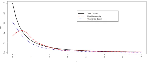
Example 3.1.1 The boundary problem can be detected in …gure (3:1). The theoretical curve is that of the pareto density.
Figure 3.1: Boundary e¤ect in kernel density estimation
3.2
Methods for removing boundary e¤ects
The properties of the classical kernel methods are satisfactory, but when the support of the variable is bounded, kernel estimates may su¤er from boundary e¤ects. Therefore, the
so-called boundary correction is needed in kernel estimation. Removing boundary e¤ects in kernel density estimation can be done in various methods. Some methods were selected which seemed to be reasonable. There were methods which were rather complicated and others which on the other hand felt quite natural.
The re‡ection method
The re‡ection method is introduced by Schuster(1985) [53], then study by Cline and Hart (1991) [14]. this method speci…cally designed for the case f0(0) = 0, where f0 denotes the …rst derivative off. Simplest way is to re‡ect the data pointsX1; :::; Xn
at the origin, just add X1; :::; Xn to the data set. This is usually referred to as
the re‡ection estimator and it can also be formulated as
b fR(x) = 1 nb n X i=1 k x Xi b +k x+Xi b ; for x 0; for x <0;fbn(x) = 0.
Transformation of data method
The transformation idea is based on transforming the original data X1; :::; Xn to
g(X1); :::; g(Xn), whereg is a non-negative, continuous and monotonically
increas-ing function from [0;1) to [0;1). Based on the transformed data, the estimator (3:1)becomes: ^ fT(x) = 1 nb n X i=1 k x g(Xi) b :
Note this isn’t really estimating the density function of X, but instead ofg(X) Pseudo-Data Methods
The pseudo-data method estimator is de…ned (see Cowling and Hall (1996) [15]), this generates data beyond the left endpoint of the support of the density.
b fCH(x) = 1 nb ( n X i=1 k x Xi b + m X i=1 k x+X( i) b ) : where X( i) = 5X(i=3) 4X(2i=3)+ 10 3 X(i); i= 1;2; :::; n;
and X(i) is theith-order statistic of sampleX1; :::; Xn, andmis an integer such that
nb < m < n.
Boundary kernel method
The boundary kernel method is more general than the re‡ection method in the sense that it can adapt to any shape of density. However, a drawback of this method is that the estimates might be negative near the endpoints; especially when f(0) 0.The boundary kernel and related methods usually have low bias but the price for that is an increase in variance. The boundary kernel estimator with bandwidth variation is de…ned (see Zhang and Karunamuni (1998) [67]) as
^ fB(x) = 1 nbs n X i=1 k(s='(s)) x Xi bs ;
where s = minfx=b;1g; k(s='(s)) is a boundary kernel satisfying k(1)(t) = k(t), and
bs ='(s)b with '(s) = 2 s: Also k(s='(s))(t) = 12 (1 +s)4 (1 +t) (1 2s)t+ 3s2 2s+ 1 2 If 1 t sg:
Re‡ection and transformation methods
The re‡ection estimator computes the estimate density based on the original and the re‡ected data points. Unfortunately, this does not always yield a satisfying
result since this estimator enforces the shoulder condition and still contains a bias of order b if the density does not ful…ll this condition. The generalized re‡ection and transformation density estimators introduce by Karunamuni and Alberts (2005) [34] and is given by b fRT(x) = 1 nb n X i=1 k x+g(Xi) b +k x g(Xi) b :
where g is a transformation that need to be determined.
We refer to Baszczy´nska(2016) [4];Karunamuni and Alberts(2005) [34]and Kolá¼cek and Karunamuni (2009) [38] for more details about this methods and for other methods see Zhang et al. (1999) [68].
Now for remove the boundary e¤ect in density estimation of heavy-tail distributions, we investigate a new class of estimators based on a transformation of set of the original data by the Champernowne distribution function.
3.3
Champernowne distribution
Buch-Larsen et.al. (2005) [7] used modi…ed Champernowne distribution to estimate loss distributions in insurance which is categorically heavy-tailed distributions. Some time it is di¢ cult to …nd a parametric model which is simple and …t for all values of claim in the insurance industry. Gustafsson et.al. (2007) [28] used asymmetric kernel density estimation to estimate actuarial loss distributions. The new estimator of density function is obtained by transforming the data using generalized Champernowne distribution function, because it produces good results in all the studied situations and it is straightforward to apply.
The original Champernowne distribution has density
f(x) = C
x (1=2) (x=M) + + (1=2) (x=M) ; x 0;
where C is a normalizing constant and ; and M are parameters. The distribution was mentioned for the …rst time in1936 by D.G. Champernowne when he spoke on The Theory of Income Distribution at the Oxford Meeting of the Econometric Society see, Champernowne (1936) [8], Champernowne (1937) [9]. Later, he gave more details about the distribution in Champernowne (1952) [10], and its application to economics. When equals to one and the normalizing constant c equals(1=2) , the density of the original distribution is simply called the Champernowne. Champernowne cumulative distribution function is de…ned onx 0and has the form
F(x) = x
x +M ;
with parameter >0; M >0, and density function is of the form
f(x) = M x
1
(x +M )2:
The Champernowne distribution converges to a Pareto distribution in the tail, while look-ing more like a lognormal distribution near0when >1. Its density is either0or in…nity at0 (unless = 1).
3.3.1
Modi…ed Champernowne distribution
We generalize the Champernowne distribution with a new parameterc. This parameter ensures the possibility of a positive …nite value of the density at0 for all .
has the form
T(x) = (x+c) c
(x+c) + (M +c) 2c ; 8x2R+;
with parameter >0; M >0 and c 0, and its density is
t(x) = (x+c)
1
((M +c) c )
((x+c) + (M +c) 2c )2; 8x2R+:
Corresponding to the Champernowne distribution, the modi…ed Champernowne distribu-tion converges to a Pareto distribudistribu-tion in the tail, for the large values ofx:
t(x)!
((M +c) c )1=
x +1 :
A crucial step when using the Champernowne distribution, is the choice of parameter estimators. As described in Buch-Larsen et al. (2005) [7], a natural way is to recognize that T(M) = 1=2 and therefore estimate the parameter M as the empirical median, and then estimate( ; c) by maximizing the log-likelihood function
l( ; c) =nlog( ) +nlog((M+c) c ) + ( 1) n X i=1 log(Xi+c) 2 n X i=1 log ((Xi+c) + (M +c) 2c ):
The choice of M as the empirical median, especially for heavy-tailed distributions, and the maximum likelihood estimates of( ; c)ensures the best over-all …t of the distribution. Remark 3.3.1 The e¤ect of the additional parameter c is di¤erent for > 1 and for
<1. The parameter c has some scale parameter properties: when <1, the derivative of the cumulative df becomes larger for increasing c, and conversely, when > 1, the derivative of the df becomes smaller for increasing c. When 6= 1, the choice of c a¤ects the density in three ways.
the opposite when >1.
Secondly,c changes the density in 0. A positive cprovides a positive …nite density in 0 : 0< t(0) = c
1
(M +c) c <1; when c >0.
Thirdly,c moves the mode. When >1, the density has a mode, and positivecshift the mode to the left. We therefore see that the parameter c also has a shift parameter e¤ect. When = 1, the choice of c has no e¤ect.
Figure 3.2: Modi…ed Champernowne distribution function, (M = 3; = 0:5) . c = 0 dashed line andc= 2 solid line.
Figure 3.3: Modi…ed Champernowne distribution function, (M = 3; = 2) . c= 0dashed line andc= 2 solid line.
3.4
Density estimation using Champernowne
trans-formation
Consider a sample random of size n, X1; :::; Xn, from unknown df, F or density
func-tionf. We will make a detailed derivation of the density estimator based on the modi…ed Champernowne distribution. This estimator is obtained by transforming the data set with a parametric estimator. The estimator of M is the empirical median and the likelihood estimator of andcare the values which maximize likelihood function and afterwards esti-mating the density of the transformed data set using the classical kernel density estimator (3:1). The estimator of the original density is obtained by back-transformation.
Lemma 3.4.1 Using transformation y=T(x), then
g(y) = f T 1(y) 1 jt(T 1(y))j;
and
f(x) = g(T(x))t(x) = g(T(x)) 1 (T 1)0(x) ; where t(x) = T0(x):
Proof. Fory=T(x); x =T 1(y) andt(x) = dT(x)
dx : The density function of variableX
isf(x)and F(x) its cumulative df. Note thatG(y) cumulative df of variable Y and g(y) its density function, then
G(y) =P (Y y) =P X T 1(y) =F T 1(y) ; and g(y) = dG(y) dy = dF (T 1(y)) dy =f T 1(y) dT 1(y) dy =f T 1(y) 1 dT(x) dx =f T 1(y) 1 jt(T 1(y))j: Forx=T 1(y); y =T(x); f(x) = g(T(x)) dT(x) dx =g(T(x))jt(x)j =g(T(x)) 1 (T 1)0(x) :
This achieves the proof of Lemma3:4:1:
Theorem 3.4.1 Given a set of data X1; :::; Xn, cumulative df T; is the modi…ed
Cham-pernowne distribution function, then
Yi =T(Xi); i= 1; :::; n;
are new variable, Yi is in the interval [0;1] and uniform distributed, then the density
function for transform data is
g(y) =f T 1(y) 1 jt(T 1(y))j:
and the formulation of the kernel density estimation for transform data Y1; :::; Yn is
e gn(y) = 1 nb n X i=1 k y Yi b ;
where k(:) is kernel function.
Boundary correction, is needed since y are in the interval [0;1], it is necessary to have a boundary correction to ensure that the kernel density estimator for transform data is a consistent estimator at the boundary. We use a simple renormalization method, as described in Jones(1993) [31]which ensures that each kernel function integrates to1. The formula kernel density estimator for transform dataY1; :::; Ynwith the boundary correction
is so e gn(y) = 1 nbky n X i=1 k y Yi b ; where ky = Z max(1;(1 y=b)) max( 1; y=b) k(u)du:
Using Theorem3:4:1 kernel density estimation for data Xi; i= 1; :::; nis;
e
fn(x) = e
gn(T (x))
j(T 1)0(x)j: The formula of transformation kernel density estimation is
e fn(x) = 1 nbkT(x) n X i=1 kb T (x) T (Xi) b T 0(x)
3.4.1
Asymptotic theory for the transformation kernel density
estimator
We investigate the asymptotic theory of the transformation kernel density estimator. Buch-Larsen et.al. (2005) [7], presented a theorem about the asymptotic theory of the transformation kernel density estimator in general (asymptotic bias and variance).
Theorem 3.4.2 Let X1; :::; Xn be independent identically distributed variables with
den-sity f. Let fen(x) be the transformation kernel density estimator of f(x)
e fn(x) = 1 nb n X i=1 k T (x) T (Xi) b T 0(x);
where T( ) is the transformation function.
Then the bias and the variance offen(x) are given by
E fen(x) f(x) = 1 2 2(k)b 2 f(x) T0(x) 0 1 T0(x) 0 +o b2 ; and V ar fen(x) = 1 nbR(k)T 0(x)f(x) +o 1 nb : as n! 1; where 2(k) = R u2k(u)dx and R(k) =R k2(u)dx.
Proof. The variable transformationYi =T(Xi) has the density g such as
g(y) = f(T
1(y))
T0(T 1(y)):
Letegn(y) be the classical kernel density estimator of g(y)
e gn(y) = 1 nb n X i=n k y Yi b :
The mean and variance of the classical kernel density estimator
E(egn(y)) =g(y) + 1 2 2(k)b 2g00(y) +o b2 ; and V ar(egn(y)) = 1 nbR(k)g(y) +o 1 nb :
The expression of the kernel estimator of density through the transformation by the stan-dard kernel estimator of density is:
e fn(x) = T0(x)egn(T (x)): Then E fen(x) =T0(x)E(egn(T (x))) =T0(x) g(T (x)) + b 2 2g 00(T (x)) 2(k) +o b2 ;
we have g(T (x)) = f(x) T0(x) g0(T (x)) = dg(T (x)) dT (x) = dg(T (x)) dx : dx dT (x) = f(x) T0(x) 0 1 T0(x); and g00(T (x)) = d dT (x)(g 0(T(x))) = d dx(g 0(T (x))) dx dT (x) = f(x) T0(x) 0 1 T0(x) 1 T0(x); E fen(x) f(x) = 1 2 2(k)b 2 f(x) T0(x) 0 1 T0(x) 0 +o b2 ; and V ar fen(x) = (T0(x)) 2 V ar(gen(T(x)) = (T0(x))2 1 nbR(k)g(y) +o 1 nb = 1 nbT 0(x)R(k)f(x) +o 1 nb :
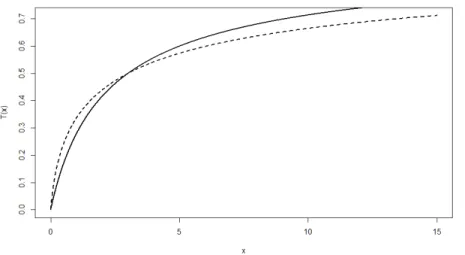
Example 3.4.1 Taking boundary problem for rv X with pareto distribution with parame-ter ( ; ) = (1;1) and sample size n = 500: Graphical output …gure (3:4) illustrates the boundary correction by the transformation method.
A modi…ed Champernowne
transformation to improve boundary
e¤ect in kernel distribution
estimation
Abstract. Kernel distribution estimators are not consistent when estimating a distribu-tion funcdistribu-tion near the boundary of its support. This problem is due to boundary e¤ects. Several solutions to this problem have already been proposed. In this paper, we propose an estimator for heavy-tailed distributions using the boundary kernel distribution estimator by transforming the data set with a modi…cation of the Champernowne distribution func-tion. The asymptotic bias, variance and mean squared error of the proposed estimator are determined. In a simulation studies, we show that the proposed method performs quite well when compared with the existing methods.
Key words: Transformation; Boundary e¤ect; Kernel distribution estimation; Mean Square Error; MeanIntegrated Equare Error.
4.1
Introduction
L
etXbe a real random variable (rv) with unknown continuous distribution function (cdf)F and density functionf. An important statistical problem is the estimation of a cdf F: A simple or the classic nonparametric estimator of the cdf is the empirical distribution function estimator. But, these estimators are step functions, and therefore, they have undesirable properties. To overcome these disadvantages, smoothing versions of them are often used. Among them kernel smoothing is most widely used because it is easy to derive and has good properties. Kernel smoothing has received a lot of attention in density estimation contex (see, e.g., Silverman (1986) [55], Wand and Jones (1995) [61]). Speci…cally, let X1; :::; Xn be a sample of size n 1 from the rv X. The popularnonparametric kernel estimator of f which is introduced by Rosenblatt (1956) [51] and Parzen(1962) [47] and has the form
b fn(x) = 1 nb n X i=1 k x Xi b ;
whereb :=bn is the bandwidth or the smoothing parameter (b !0, as n ! 1) and k
is a nonnegative symmetric kernel function such that it is bounded and has …nite support. The kernel distribution function estimator Fbn(x) was proposed by Nadaraya (1964) [45].
Such an estimator arises as an integral of the Parzen-Rosenblatt kernel density estimator (see Reiss(1981) [49] and Tenreiro (2013)) [57]and is de…ned for x2R; by
b Fn(x) = Z x 1 b fn(t)dt= 1 n n X i=1 K x Xi b ; (4.1) where K(x) := Z x 1 k(t)dt;
is the integrated kernel. However, several properties of Fbn(x) have been investigated,
b
Fn(x); and determined also the asymptotically optimal smoothing parameter. Winter
(1979) [65] and Yamato (1973) [66] proved the uniform convergence of Fbn(x) to F(x)
with probability one, the asymptotic normality of Fbn(x) is established by Watson and
Leadbetter(1964) [62].
The problems of boundary e¤ect for kernel estimators with compact supports is well-known in regression and density function estimation and several modi…ed estimators have been proposed in the literature (see Gasser and Müller(1979) [25], Karunamuni and Al-berts(2005) [34], Zhang and Karunamuni (1999) [68], and references therein). A similar correction would be made for improve the theoretical performance of the usual kernel distribution function estimator (4:1); at the boundary points. More speci…cally the per-formance ofFbn(x)at boundary points, forx2[0; b][(a b; a];0< a 1;however di¤ers
from the interior points due to so-called “boundary e¤ects” that occur in nonparametric curve estimation problems. The bias ofFbn(x)is of ordero(b)instead of o(b2)at boundary
points, while the variance of Fbn(x) is of order o
b
n . This fact can be clearly seen by
examining the behavior of Fbn inside the left boundary region [0; b]. Let x be a point in
the left boundary region,x 2[0; b]. The bias and variance of Fbn(x) at x=sb; 0 s 1
are Bias Fbn(x) =bf(0) Z s 1 K(t)dt (4.2) +b2f0(0) s 2 2 +s Z s 1 K(t)dt Z s 1 tK(t)dt +o b2 ; and V ar Fbn(x) = F(x) (1 F(x)) n + b nf(0) Z s 1 K2(t)dt s +o b n : (4.3)
To remove those boundary e¤ects in kernel distribution estimator, a variety of methods have been developed in the literature. We brie‡y mention re‡ection of data (see, e.g.,
Silverman(1986) [55]), transform of data (see, Marron and Ruppert(1994) [42]), pseudo-data method (see Cowling and Hall (1996) [15]) and also the boundary kernel method (Gasser et al. (1985) [26], Zhang and Karunamuni (2000) [69]). For more details about this techniques one refers to Karunamuni and Alberts (2005)[34]; Karunamuni and Alberts (2004) [33].
In this paper, we develop a new kernel type estimator of the heavy-tailed distributions functions that improved boundary e¤ects near the points at left boundary region, for
x2[0; b]. This estimator is based on a new transformation on boundary corrected kernel estimator ideas of Kolá¼cek and Karunamuni (2009) [38]; Buch-Larsen et al. (2005) [7], developed for boundary correction in kernel density estimation. The basic technique of construction of the proposed estimator is kind of a generalized re‡ection method involving re‡ecting a transformation of the observed data, we used two transformations. First, a transformationg is selected from a parametric family, second we propose to use a transfor-mationT based on the little-known Champernowne distribution function, which produces good results in all situations studied and it is straightforward to apply.
Theoretical properties of boundary kernel distribution estimator are introduced in Section 4:2. In Section4:3the proposed estimator is given and its bias and variance are computed. In Section 4:4, simulation studies are done to see the performance of the proposed esti-mator, and compare it with the "usual" and "boundary" distribution function estimators. Finally, all Proofs are referred to Section4:5.
4.2
Boundary kernel distribution estimator
In order to deal with the boundary e¤ects that occur in nonparametric regression and density function estimation, the use of boundary kernels is proposed and studied by authors such as Gasser and Müller (1979) [25], Karunamuni and Alberts (2004) [33]. Next we extend this approach to a distribution function estimator framework. The structure of this
estimator is the same type of that in density estimation case which has been discussed in Karunamuni and Alberts(2007) [35], for more details see Zhang and Karunamuni (1999) [68]. This method of estimating combines the transformation and the re‡ection methods, consisting of three steps:
Step 1: Transform the initial data X1; :::; Xn to g(X1); :::; g(Xn); where g is a nonnegative,
continuous, and monotonically increasing function from [0;1)to [0;1): Step 2: Re‡ect g(X1); :::; g(Xn) around the origin, so we get g(X1); :::; g(Xn):
Step 3: The estimator ofF is based on the enlarged data sample g(X1); :::; g(Xn); g(X1); :::; g(Xn):
Then the boundary kernel distribution estimator of the distribution function for
x2[0; b]; is given by Fn(x) = 1 n n X i=1 K x g(Xi) b K x+g(Xi) b ; (4.4)
where K is a distribution of the kernel function k as in (4:1).
This estimator generates a class of boundary corrected estimators. We need to obtain explicit forms of the bias, variance and asymptotic mean square error expressions of the estimator (4:4).
Lemma 4.2.1 Assume that f0(:) and g00(:) exist and are continuous. Further, assume
that g 1(0) = 1 and g0(0) = 0; where g 1 the inverse function of g and f0 and g00 are the
…rst and second derivatives of f and g respectively. Then for x=sb; 0 s 1; we have
Bias Fn(x) =b2 f0(0) s2 2 + 2s Z s 1 K(t)dt Z s s tK(t)dt f(0)g00(0) Z s 1 (s t)K(t)dt+ Z s 1 (s+t)K(t)dt +o b2 ; (4.5)
and V ar Fn(x) = F(x) (1 F(x)) n + b nf(0) 2 Z s 1 K2(t)dt s + Z s s K2(t)dt 2 Z s 1 K(t)K(t 2s)dt +o b n : (4.6)
Accordingly, the asymptotic mean squared error is
AM SE Fn(x) =b4 f0(0) s2 2 + 2s Z s 1 K(t)dt Z s s tK(t)dt f(0)g00(0) Z s 1 (s t)K(t)dt+ Z s 1 (s+t)K(t)dt 2 + F(x) (1 F(x)) n + b nf(0) 2 Z s 1 K2(t)dt s + Z s s K2(t)dt 2 Z s 1 K(t)K(t 2s)dt : (4.7) Remark 4.2.1 Functions satisfying conditions g 1(0) = 1 and g0(0) = 0 are easy to construct. The trivial choice isg(y) =y, which represents the “classical”re‡ection method estimator. The following transformation adapts well to various shapes of distributions:
g(y) =y+ 1 2Isy
2; for y 0 and 0 s 1; where Is=
R s
1 K(t)dt:
Remark 4.2.2 Some discussion on the above choice of g and other various improvements that can be made would be appropriate here. It is possible to construct functions g that improve the bias under some additional conditions. For instance, if one examines the right hand side of bias expansion, then it is not di¢ cult to see that the coe¢ cient ofb2 can be made equal to zero if g is appropriately chosen, (see Kolá¼cek and Karunamuni (2009) [38]).