Phase–amplitude coupling and the BOLD signal: A simultaneous intracranial EEG (icEEG) - fMRI study in humans performing a finger-tapping task

Phase

–

amplitude coupling and the BOLD signal: A simultaneous

intracranial EEG (icEEG) - fMRI study in humans performing

a

fi

nger-tapping task

T. Murta

a,b,n

, U.J. Chaudhary

a

, Tim M. Tierney

c

, A. Dias

b

, M. Leite

a,b

, D.W. Carmichael

c

,

P. Figueiredo

b

, L. Lemieux

a

a

Dept. of Clinical and Experimental Epilepsy, UCL Institute of Neurology, London, United Kingdom

b

Institute for Systems and Robotics and Department of Bioengineering, Instituto Superior Técnico, Universidade de Lisboa, Lisboa, Portugal

c

UCL Institute of Child Health, London, United Kingdom

a r t i c l e i n f o

Article history: Received 12 April 2016 Accepted 18 August 2016 Keywords: Intracranial EEG fMRI

Phase–amplitude coupling Electro-haemodynamic coupling

a b s t r a c t

Although it has been consistently found that local blood-oxygen-level-dependent (BOLD) changes are better modelled by a combination of the power of multiple EEG frequency bands rather than by the power of a unique band alone, the local electro-haemodynamic coupling function is not yet fully char-acterised. Electrophysiological studies have revealed that the strength of the coupling between the phase of low- and the amplitude of high- frequency EEG activities (phase–amplitude coupling - PAC) has an important role in brain function in general, and in preparation and execution of movement in particular. Using electrocorticographic (ECoG) and functional magnetic resonance imaging (fMRI) data recorded simultaneously in humans performing afinger-tapping task, we investigated the single-trial relationship between the amplitude of the BOLD signal and the strength of PAC and the power of

α

,

β

, and

γ

bands, at a local level. In line with previous studies, we found a positive correlation for the

γ

band, and negative correlations for the PAC_βγstrength, and the

α

and

β

bands. More importantly, we found that the PAC_βγ strength explained variance of the amplitude of the BOLD signal that was not explained by a combination of the

α

,

β

, and

γ

band powers. Our mainfinding sheds further light on the distinct nature of PAC as a functionally relevant mechanism and suggests that the sensitivity of EEG-informed fMRI studies may increase by including the PAC strength in the BOLD signal model, in addition to the power of the low- and high- frequency EEG bands.

&2016 The Authors. Published by Elsevier Inc. This is an open access article under the CC BY license (http://creativecommons.org/licenses/by/4.0/).

1. Introduction

In the last century, human brain activity has been recorded most commonly as electrical potentials on the scalp (scalp electroencephalography EEG), neocortex (electrocorticography -ECoG), or inside the brain (depth EEG). Since the early 1990s, re-cording changes in the local blood oxygenation, using blood-oxy-gen-level-dependent (BOLD) functional magnetic resonance ima-ging (fMRI), has become an increasingly important tool, largely due to its non-invasive whole-brain coverage and relatively high spatial resolution. However, notwithstanding numerous studies on the electrophysiological correlates of the BOLD effect, our under-standing of the coupling between EEG and BOLD signals remains limited (Valdes-Sosa et al., 2009;Murta et al., 2015).

Since the discovery of EEG, a range of rhythmic activities characteristically associated with sensory, motor, and cognitive events, has been observed on its recordings (Engel et al., 2001;

Varela et al., 2001;Jacobs and Kahana, 2010). These activities

ap-pear to hierarchically interact with each other, as the“basic units”

of a complex system that regulates information processing in the brain, across multiple spatial and temporal scales (Lakatos et al.,

2005;Palva et al., 2005;Roopun et al., 2008;Canolty and Knight,

2010;Buzsaki et al., 2012;Hyafil et al., 2015). The influence of the

phase of the low-frequency (LF) activity in the amplitude of the high-frequency (HF) activity, a phenomenon called phase– ampli-tude coupling (PACLF HF), has attracted great interest due to its

potential functional role (Kramer et al., 2008;Lakatos et al., 2008;

Cohen et al., 2009a,2009b;Tort et al., 2009;Axmacher et al., 2010;

Buzsáki et al., 2012). In the human motor cortex, EEG activity

above 40 Hz is increased during movement, whereas

α

(8–14 Hz) and

β

(14–30 Hz) activities tend to be decrease during its execu-tion, in comparison to rest (Crone et al., 1998;Miller et al., 2012). Fluctuations in PAC_αγ and PAC_βγ have also been linked to Contents lists available atScienceDirect

journal homepage:www.elsevier.com/locate/neuroimage

NeuroImage

http://dx.doi.org/10.1016/j.neuroimage.2016.08.036

1053-8119/&2016 The Authors. Published by Elsevier Inc. This is an open access article under the CC BY license (http://creativecommons.org/licenses/by/4.0/). n_{Corresponding author at: UCL Institute of Neurology, Department of Clinical}

and Experimental Epilepsy, 33 Queen Square BOX 29, WC1N 3BG London, United Kingdom.

movement execution and pre- and/or post- movement rest (Miller

et al., 2012;Yanagisawa et al., 2012).

With regard to fMRI, it has been found that EEG powerfl uc-tuations in the

α

,

β

, and

γ

bands explain independent, as well as common, components of the BOLD signal amplitude variance

(Scheeringa et al., 2011;Magri et al., 2012). Many studies have also

investigated the relationship between multi-unit activity (MUA), localfield potentials (LFP) and the BOLD signal. While some found that both MUA and LFP were equally good correlates of the BOLD signal amplitude (Mukamel et al., 2005;Nir et al., 2007), others found that LFP accounted for significantly larger amounts of its variance (Logothetis and Wandell, 2004). It is currently accepted that the BOLD signal reflects both LFP and MUA, to different de-grees, depending on the conditions (Ekstrom, 2010). Of particular relevance to us is the observation byWhittingstall and Logothetis

(2009)who found that the

γ

band power was a good predictor of

MUA only when its increases were time-locked to a certain

δ

phase, suggesting that a particular interaction between the phase and the amplitude of different bands may predict MUA better, and it may therefore also be related to the BOLD signal differently.

In summary, (i)fluctuations in

α

,

β

, and

γ

band power, and in PAC_αγand PAC_βγ strength, are reflections of the brain state; (ii) fluctuations in the power of multiple frequency bands predict BOLD changes better thanfluctuations in the power of the

γ

band alone; (iii) LFP and MUA predict BOLD changes differently, de-pending on the conditions; and (iv) PACfluctuations predict MUA better than LFP

γ

powerfluctuations alone.

In this study, we used ECoG and fMRI data simultaneously re-corded in humans performing afinger-tapping task to investigated how single-trialfluctuations in the PAC strength relate to the co-localised single-trial fluctuations in the amplitude of the BOLD signal; in particular, to investigate whetherfluctuations in the PAC strength explained variance of the BOLD signal amplitude that was not explained by a combination of

α

,

β

, and

γ

band powers. Using invasive EEG recordings (ECoG, depth EEG) is a way to surpass one of the major limitations of scalp EEG - the presence of the skull between the recording site and the active neuronal tissue that acts as a low-passfilter of the electricalfield potential, which therefore allowed to record EEG activity above 70 Hz reliably. It is also a way to guarantee that we are investigating the relationship between the electrophysiological and haemodynamic responses at a local level (the responses under investigation are most likely to be generated by the same brain region). Furthermore, using invasive EEG and fMRI data simultaneously recorded is the only way to guarantee that we are analysing responses related to the same (neuronal) phenomenon. Single-trial variability due to different performances, habituation effects, plasticity, or uncontrolled var-iations in the response to the stimulation paradigm cannot be investigated using data sequentially acquired (Villringer et al., 2010). More importantly, the patient’s determination and physical capability to perform the task exactly when asked to do it do not affect dramatically studies using data simultaneously acquired but they do affect studies using sequentially acquired data, which potentially results in a lower correlation between the two sponses that is not explained by their decoupling. We have re-cently used this type of data to study the BOLD correlates of sharp waves; we found that the amplitude of the BOLD signal depends more on the duration of the underlyingfield potential (reflected in the sharp wave width) than on the degree of neuronal activity synchrony (reflected in the sharp wave amplitude) (Murta et al, 2016). To the best of our knowledge, this is the first study in-vestigating single-trial correlations between the strength of PAC, estimated from human ECoG data, and the amplitude of the BOLD signal simultaneously recorded, at a local level.

2. Methods 2.1. Patient selection

Intracranial EEG (icEEG) and fMRI data were simultaneously recorded in patients (of either sex) with severe drug-resistant epilepsy, who underwent invasive EEG monitoring as part of their pre-surgical evaluation. The implantation scheme and electro-physiological (depth EEG and/or ECoG) data acquired varied across patients, depending on their clinical history and surgical con-siderations. In total, seven patients had part of or the whole motor cortex covered by subdural strips and/or grids. The icEEG-fMRI data were acquired with the written informed consent of patients, as part a project approved by the Joint UCL/UCLH Committees on the Ethics of Human 107 Research, at the neuroradiology depart-ment of the National Hospital for Neurology and Neurosurgery in London, following strict guidelines (Carmichael et al., 2008,2010). 2.2. Simultaneous acquisition of icEEG and fMRI data

The icEEG-fMRI acquisition consisted of two 10 min resting state runs and a 5 min motor task run. In this study, we focus entirely on the latter. Six patients alternatively tapped their left-and right-fingers, in blocks of 30 s each. In two cases, thefi nger-tapping blocks were interleaved with 30 s blocks of rest. The se-venth patient performed the same task, with rest, using his feet. The simultaneous icEEG-fMRI data acquisition protocol is de-scribed inCarmichael et al. (2012).

The MRI data was acquired on a 1.5 T scanner (TIM Avanto, Sie-mens, Erlangen, Germany), with a quadrature head transmit–receive radio-frequency (RF) coil using low specific absorption rate se-quences (o0.1 W/kg head average), simultaneously with icEEG data, in accordance with our acquisition protocol (Carmichael et al. 2012). The fMRI scan consisted of a gradient-echo echo-planar imaging (GE-EPI) sequence with the following parameters: TR/TE/flip angle_¼3000 ms/40ms/90_°, 6464 acquisition matrix, 382.5 mm slices with 0.5 mm gap. In addition, a FLASH T1 weighted structural scan was acquired with the following parameters: TR/TE/flip angle_¼15 ms/4.49 ms/25_°, resolution 1.01.21.2 mm, FoV 260211170 mm, 256176142 image acquisition matrix with the readout direction lying in the sagittal plane; scan duration: 6 min 15 s.

Details on safety concerns of recording icEEG data simulta-neously with fMRI data and on fMRI data quality were previously discussed inCarmichael et al. (2010)andCarmichael et al. (2012), respectively.

IcEEG data were acquired with an MR-compatible system (Brain Products, Gilching, Germany) and respective software (Brain Recorder, Brain Products, Gilching, Germany), at a 5 kHz sampling rate. The icEEG recording system was synchronised with the 20 kHz gradient MR scanner clock.

The computed tomography (CT) data was acquired with a Sie-mens, SOMATOM Definition ASþscanner, with a 0.430.431mm resolution and a 512512169 image matrix, shortly after the implantation of the icEEG electrodes and prior to the icEEG-fMRI acquisition, as part of the patients' clinical management.

2.3. Pre-processing of icEEG and fMRI data

SPM12 (http://www.fil.ion.ucl.ac.uk/spm/software/spm12/) was used to realign and spatially smooth (using an isotropic 5 mm FWHM Gaussian kernel) the fMRI data. Prior to smoothing, phy-siological noise was removed from the fMRI data using FIACH (Functional Image Artefact Correction Heuristic) (Tierney et al., 2015). In brief, FIACH is a two-step biophysically-based approach designed to identify brain regions that show high temporal

instability and to remove large amplitude temporal BOLD signal changes of non-neuronal origin. Based on the fMRI signal from the brain regions identified in the first step, FIACH generates 6 re-gressors that reflect physiological noise and can be included in the GLM as confounds.

After removing the MR acquisition-related artefacts from the icEEG data using an average template subtraction approach (Allen

et al., 2000), the icEEG data were down-sampling to 500 Hz. No

hearbeat-related artefact correction was necessary as previously reported (Carmichael et al., 2012).

In this study, we use the specific terms ECoG or depth EEG rather than the generic term icEEG to refer to the electro-physiological signal when suitable.

Bipolar icEEG time courses were obtained for every pair of adjacent icEEG contacts by subtraction of the voltage of the more posterior contact from that of the more anterior one.

2.4. Functional MRI motor function mapping and the BOLD time-course of interest

A square wave function corresponding to the periods of con-tralateral (to the icEEG contacts) finger tapping was convolved with the canonical HRF and used as regressor of interest in a whole-brain general linear model (GLM) analysis of the pre-pro-cessed fMRI data. The following confounding effects were also included in this model, as regressors of no interest: 24 movement related confounds (6 realignment parameters, and their Volterra expansion (Friston et al., 1996)), and 6 fMRI physiological noise related confounds (Tierney et al., 2015). A square-wave function representing periods of ipsilateral (to the icEEG contacts)finger tapping was convolved with the canonical HRF and also included in the model, in the cases wherefinger tapping was interleaved with rest. All GLM were estimated using SPM12 (http://www.fil.

ion.ucl.ac.uk/spm/software/spm12/).

A positive t-contrast for the regressor of interest was used to localise the BOLD changes positively correlated with the con-tralateral (to the icEEG contacts)finger tapping. The corresponding statistical parametric maps were thresholded at po0.001, un-corrected, and the resulting cluster with a minimum extent of 10 voxels, located in the motor cortex, was used as the region of in-terest (ROI) for the subsequent analyses. The BOLD signal time-course of interest was obtained by averaging the time-time-courses across the ROI voxels, and high-passfiltering the resulting time-course using a Butterworthfilter of order 4 and cut-off frequency of 1/128 Hz (Matlab functionbutter), to remove the slow drift. 2.5. Contacts, frequency bands, and features of interest for BOLD modelling

This section describes various steps taken in the generation of the ECoG-derived features of interest, which were subsequently compared in terms of their capability to predict the co-localised finger-tapping related BOLD changes, i.e. the BOLD time course of interest.

We used the classical

α

(8–14 Hz),

β

(14–30 Hz), and

γ

(70–

182 Hz) bands (Lopes da Silva, 2011) to identify the ECoG contact pairs that showed the largest task-related

α

,

β

, and

γ

power fluctuations (Miller et al., 2012); these were the contact pairs of interest - COI_α, COI_β, COI_γ, and their search is further described in

2.5.1Nevertheless, in the following steps of this study, we used

patient-specific

α

and

β

bands, narrower than the classical bands, centred at patient-specific frequencies (Aru et al., 2014), and mainly containing rhythmic activity; their central frequencies were found as described in2.5.2. Then, for each patient showing both significantfinger tapping BOLD changes and a significant PAC effect, one or two (depending on whether the PAC effect was

significant) PAC strength regressors - PAC_αγand/or PAC_βγ- were computed, as described in2.5.3.

2.5.1. Contacts of interest (COI)

For each patient and ECoG contact pair located over the motor cortex (seeTable 1for a schematic illustration of these contacts), we computed the power spectra (using the Matlab function fft) over the two finger tapping periods: ipsilateral (to the icEEG contacts) _finger tapping, Sipsi

_{( )}

f , and contralateralfinger tapping,

( )

Scontr f . Then, for each frequency band of interest,fb= [f1, 2f ], we computed the difference between the areas under the two power spectra,∆Sfb, as: ⎛ ⎝ ⎜ ⎜ ⎞ ⎠ ⎟ ⎟

( )

( )

∑

∑

∆ = − ∆ ( ) = = S S f S f f 2-1 fb f f f contr f f f ipsi 1 2 1 2

where∆fis the sampling frequency. The patient-specific COI were defined as those showing the largest∆Sα,∆Sβ, and∆Sγ, and were labelled COI_α, COI_β, and COI_γ, respectively. Here,

α

and

β

were defined as the classical [8–14] Hz and [14–30] Hz frequency bands

(Lopes da Silva, 2011), and

γ

as [70–182] Hz.

2.5.2. Patient-specific frequency bands

Following the identification of the patient-specific COI_α, COI_β, and COI_γ, we identified the central frequencies of the task-related and patient-specific

α

and

β

rhythmic activities in the harmonic component of the ECoG power spectrum. For each patient, we performed a coarse-graining spectral analysis (CGSA) (Yamamoto

and Hughson, 1991) to isolate the fractal and harmonic

compo-nents of the COI_αand COI_βpower spectra (He et al., 2010); CGSA was applied to the blocks of ipsilateral (to the ECoG implantation) finger tapping to take advantage of the stronger

α

and

β

rhythmic activities during these periods.

First, the ECoG time course was segmented into 5 s non-over-lapping epochs, which were multiplied by a Hanning window of the same length (obtained with the Matlab function hann), de-meaned, and called x i( ). Second, x t( ), x t2( ), and x1/2( )t, were computed as: ( )= ( )( = … ) ( ) x t x i i 1, 2, 3, , /2N 2-2 ( ) = ( )( = … ) ( ) x t2 x i i 2, 4, 6, ,N 2-3 ( )= ( )( = … ) ( ) x1/2t x i i 1, 1, 2, 2, 3, 3, , /4N 2-4 where N is the number of data samples within each 5 s epoch.

( )

x t2 , andx1/2( )t are called the coarse-grained time courses. Third, the auto-power spectrum of x t( ),Sxx, the cross-power spectrum of

( )

x t and x t2( ), Sxx₂, and the cross-power spectrum of x t( ) and

( )

x1/2t, Sxx_1/2, were obtained using Matlab functionsxcorrandfft.

Finally, the raw, the fractal, and the harmonic power spectra were computed as:

∑

( ) = ( ) ( ) = S f raw M S f 1 2-5 m M xx 1

∑

∑

( ) = ( )∙ ( ) ( ) = = S f fractal M S f M S f 1 1 2-6 m M xx m M xx 1 1 2 1/2

( )

=

( )

−

( )

( )

S f harmonic S f raw S f fractal 2-7 where Mis the number of epochs.

For each patient, the centre of the

α

band was chosen to be the frequency showing the maximum power in the band [8–14] Hz of the COI_αharmonic power spectrum, and its width to be 2 Hz; and the centre of the

β

band was chosen to be the frequency showing the maximum power in the band [14–30] Hz of the COI_βharmonic power spectrum, and its width to be 6 Hz (Aru et al., 2014). The

γ

band was kept as [70_–182] Hz because no obvious peak was found in this frequency band of the COI_γharmonic power spectrum.

2.5.3. ECoG-derived BOLD predictors

In this section, we describe how the ECoG time courses were processed for PAC calculation, and how two PAC strength re-gressors, PAC_αγand PAC_βγ, were built for each patient.

2.5.3.1. Band-pass filtering and Hilbert transform. As a necessary step for the computation of all the ECoG-derived features in-vestigated in this study, the ECoG signals were band-passfiltered and Hilbert transformed.

The ECoG time courses were band-passfiltered using a 2-way-least squares Finite Impulse Response filter (EEGlab toolbox

(http://sccn.ucsd.edu/eeglab/) function eegfilt), chosen because it

limits phase distortion to a minimum (the input data was pro-cessed in both the forward and reverse directions). For the

α

and

β

ranges, the central frequencies of thefilters were 8, 9, 10,…, 30 Hz (sampled at every 1 Hz), and their bandwidths were set to 1 Hz, to ensure a precise estimation of the instantaneous phase (Berman

et al., 2012; Aru et al., 2014). For the

γ

range, the central

fre-quencies were 70, 74, 78…, 182 Hz (sampled at every 4 Hz), and their bandwidths were set to 60 Hz, twice the fastest

β

compo-nent, i.e. 30 Hz, to preserve the modulation that the instantaneous phase of

β

could have in the amplitude of

γ

(Berman et al., 2012;

Aru et al., 2014).

Each band-passed ECoG time course was then transformed in the complex signal _{x t}( )= ( )_{A t e}iφ( )t_{, using the Hilbert transform}

(Matlab functionHilbert), whereA t( )is the amplitude and φ( )t is the instantaneous phase ofx t( ).

Table 1

EcoG implantation characterisation: types of electrodes, number of contacts per electrode, and implantation scheme. The ECoG contact pairs analysed (over the motor cortex) are highlighted with numbered black squares. FLE: Frontal lobe epilepsy, R: right, L: left, A: anterior, M: medial, P: posterior, I: inferior, and S: superior.

Implantation scheme

Patient ID 1

Type of epilepsy FLE Anatomical location of

electrodes

- L pre/postcentral gyrus - L supramarginal gyrus - I (IFG) and M (MFG) frontal gyri

Type of electrodes two 6-contact strips, one 8x8 contact grid, one 2x8 contact grid

Patient ID 2

Type of epilepsy FLE Anatomical location of

electrodes

- L frontal lobe (laterally and inferiorly) - L M (MFG) and I (IFG) frontal gyri - L temporal lobe

Type of electrodes one 6x8 contact grid, two 2x8 contact grids, one 4x8 high-density contact grid, two 6-contact strips, two 6-contact depths

Patient ID 3

Type of epilepsy FLE Anatomical location of

electrodes

- L frontal and parietal convexity - L frontal pole

- L S frontal gyrus (SFG) - L I frontal gyrus - L mesial frontal surface

Type of electrodes one 8x8 contact grid, one 2x8 contact grid, one 8-contact strip, one 6-contact strip, one high-density 4x8 contact grid

2.5.3.2. Phase–amplitude coupling (PAC) strength. The PAC strength was computed as proposed by Canolty et al. (2006), using the Matlab code made available online (Canolty et al. (2006) supple-mentary material). Let us define a composite signal xcomposite

_{( )}

t that combines the phase of a particular low-frequency component (LF), φLF

_{( )}

t , with the amplitude of a particular high-frequency,

( )

AHF t, such that:

( )

₌

( )

φ ( ) _{( )}

xcomposite t AHF t eiLF t 2-8 The raw strength of the coupling betweenAHF( )t andφLF( )t in a

particular epoch comprising T data samples was computed as:

∑

∑

= ( )= ( ) φ _{( )} = = ( ) Mraw 1/T _t x t 1/T A t e _2-9 T composite _t T HF i t 1 1 LF

The z-scored strength of the coupling betweenAHF( )t andφLF( )t

was computed as the difference between Mrawand the mean of a

distribution of surrogates of xcomposite, obtained by jittering AHF( )t

and φLF( )t by 200 random time lags, divided by the standard de-viation of the same distribution of surrogates (Canolty et al., 2006). The mean and standard deviation of the distribution of surrogates were obtained using the Matlab functionnormfit. The z-scored PAC strengths were the subject of the subsequent analyses.

2.5.3.3. PAC- and band power- based BOLD predictors. Two PAC strength- and three power- based regressors were built for BOLD modelling: PAC_αγ, based on the

α

phase -

γ

amplitude coupling computed at COI_α; PAC_βγ, based on the

β

phase -

γ

amplitude coupling computed at COI_β; P_α, based on the

α

band power computed at COI_α; P_β, based on the

β

band power computed at COI_β; P_γ, based on the

γ

band power computed at COI_γ.

The computation of each PAC regressor involved: (i) the seg-mentation of COI_αand COI_βamplitude and phase complete time courses (Section 2.5.3.1) into 15 s overlapping epochs (5 TR), centred at the simultaneous BOLD signal epoch, (ii) the compu-tation of a PAC strength estimate for each epoch; and (iii) the concatenation of the resulting PAC strength estimates, which re-sulted in a PAC strength regressor with the temporal resolution of the_finger-tapping BOLD time course, i.e., 3 s (Fig. 1B).Tort et al.

(2010)argued that 200 cycles of the low frequency of interest (that

giving the phase) were enough to provide a reliable PAC strength estimate (in their particular experimental settings). We choose to use 15 s epochs, i.e., 120 cycles for the lower

α

component of in-terest (8 Hz), and 450 cycles for the higher

β

one (30 Hz). This seemed a good compromise between the accuracy of the PAC strength estimate (likely to increase with the number of cycles averaged) and the temporal smoothing (a consequence of the overlap).

The PAC strength metric proposed byCanolty et al. (2006)can be used to compute the strength of the coupling between a fre-quency pair, formed by the LF ECoG component giving the phase and the HF ECoG component giving the amplitude. After applying it to multiple frequency pairs, in parallel, the resulting z-scored PAC strengths (z-axis) can be plotted as a function of the LF giving the phase (x-axis) and the HF giving the amplitude (y-axis), in a form that it is often called the“phase–amplitude comodulogram”

plot. In this study, these plots were used to improve the SNR of the PAC estimates. For this, they were computed using the patient specific- COI_αand COI_βcomplete ECoG time courses (5 min). Then, the PAC strength time courses whose frequency pairs showed a significant PAC (po0.05; Bonferroni corrected for the dimensions of the frequency space) were averaged, which resulted in two average PAC strength time courses per patient. Finally, these two PAC strength time courses were convolved with the canonical HRF, which resulted in the two PAC strength regressors of interest, PAC_αγand PAC_βγ, respectively.

The power regressors of interest,P_α,P_β, andP_γ, were obtained by: (i) averaging the power time courses over the corresponding patient-specific frequency bands and COI; (ii) convolving the average power time courses with the canonical HRF, and (iii) down-sampling the result to a 3 s (¼TR) time resolution by averaging the power within each 3 s epoch.

2.6. BOLD model definition

We used the GLM framework to estimate the variance of the amplitude of the co-localisedfinger-tapping related BOLD changes, explained by each individual ECoG-derived effect (PAC, P_α, P_β, and P_γ), in turn, which was not explained by a combination of the other regressors (e.g.: PAC vs [ P_αP_βP_γ]).

We aimed to investigate the variance of the amplitude of the BOLD signal explained by the strength of PAC_αγ and PAC_βγ in-dividually in addition to the standard model, i.e., that comprising the

α

,

β

, and

γ

power derived BOLD predictors. Eight independent models were built, four for each PAC-based regressor of interest (PAC_αγ and PAC_βγ). Each model included a PAC-based regressor (PAC_αγor PAC_βγ); 3 ECoG power-based regressors (P_α, P_β, and P_γ); and 30 confounding effects (C) (24 movement-related confounds (6 realignment parameters and their Volterra expansion (Friston

et al., 1996)), and 6 fMRI physiological noise related confounds

(Tierney et al., 2015). For example, the four linear models used to

investigate thePAC_αγeffect were defined as follows:

(

)

(

)

(

)

(

)

β β β β β = × ⊗ + × ⊗ + × ⊗ + × ⊗ + +ϵ _{( )} αγ α β γ αγ α β γ y PAC HRF P HRF P HRF P HRF C _3-10 PAC P P P c

where ×, represents the product, ⊗, the convolution operation, y, the time course of the amplitude of thefinger tapping BOLD signal (obtained as described in 2.4), HRF, the canonical HRF, C, the confounding effects matrix, ϵ, the error, β, the linear coefficients estimated for each regressor included in the model (PACαγ,Pα,Pβ,Pγ,

C), PACαγ, the time course of the strength of PACαγ, Pα, the time course of the power of

γ

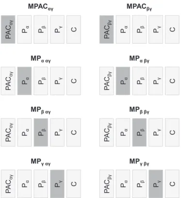
, etc…The models were labelled: MPACαγ, MP_α,αγ, MPβ,αγ, MPγ,αγand MPACβγ, MPα,βγ, MPβ,βγ, MPγ,βγ, and

their design matrices are illustrated inFig. 2, where the regressor of interest, i.e. the regressor that was orthogonalised with respect to the combination of the others, is highlighted in dark grey. This or-thogonalisation was necessary to assure that we were estimating the amount of variance that was explained by a particular regressor but not by a set of others. Note that (1) all eight models have the same exact number of regressors, and (2) each set of four models (one set for PAC_αγ, other for PAC_βγ) explains the same variance of the BOLD signal amplitude (the only difference being the way this explained variance is distributed among the regressors).

All models were estimated using the Matlab functionglmfit.

3. Results

3.1. Functional MRI motor function mapping and the BOLD time-course of interest

At least one cluster of statistically significant finger tapping-related BOLD changes was found in the primary motor cortex of 3/ 7 patients (Fig. 3), allowing us to define an appropriate ROI for the following investigations. In these 3 patients, the task consisted of interleaved right- and left-finger tapping, without rest. The data from the other 4 patients were not further analysed. The icEEG implantations are illustrated inTable 1, where the black squares show the ECoG contact pairs over the motor cortex used for the analysis (bipolar montage). The relative location of the significant cluster and ECoG contacts analysed is illustrated inFig. 4A.

3.2. Contacts, frequency bands, and features of interest for BOLD modelling

3.2.1. Contacts of interest (COI)

A schematic illustration of the ECoG contacts analysed is shown

in Table 1. The contacts pairs highlighted with black squares in

Table 1 correspond to those represented as coloured squares in

Fig. 4B (each square represents an ECoG time course). The COI

identified for each patient and frequency of interest are high-lighted with white rectangles inFig. 4A, and white circles in the scheme shown in Fig. 4B. The magnitude of the difference be-tween the area under the spectrum for the contralateral (to the ECoG contacts) and ipsilateralfinger-tapping periods varied con-siderably across the motor cortex of each patient for all frequency

bands of interest, as shown by the colour scale inFig. 4B. As ex-pected, the sign of these differences was positive for

γ

, and ne-gative for

α

and

β

.

3.2.2. Patient-specific frequency bands

The fractal and harmonic power spectra, obtained for the COI_α and COI_βof each patient, and the respective

α

,

β

, and

γ

power peaks, marked with a black arrow, are shown inFig. 5.

3.2.3. ECoG-derived BOLD predictors

The z-scored PAC strength values for the frequency-pairs that showed a significant PAC effect (po0.05; Bonferroni correction) are shown inFig. 6. No significant PAC effect was found for the

α

band of patient 1 and 3. Therefore, no PAC_αγ regressors were

A

3s

Time

…

…

…

…

BOLD time course

ECoG time course (

,

( )

)

…

…

PAC time course

Find the patient- and frequency- specific contact pairs (COI) of interest

Find the patient-specific frequency bands

Compute ECoG amplitude and phase time courses

Compute ECoG

power time courses

Compute

power-based regressors

(P

α

, P

β

, P

γ

)

Compute

comodulatgram plots

Compute PAC-based regressors

(PAC

αγ

, PAC

βγ

)

Compute ECoG

PAC time courses

Build the BOLD signal model

B

Fig. 1.Schematic illustration of the processing steps used to build the BOLD signal model based on the ECoG signal.APAC and power regressors computation pipeline. BRelationship between ECoG, PAC and BOLD time courses.

defined for these patients and only their PAC_βγ regressors were considered in the subsequent analyses.

3.3. BOLD model definition

The t-values obtained for the PAC_βγ, P_α, P_β, and P_γeffects, after estimating the models MPAC_βγ, MP_α,_βγ, MP_β,_βγ, MP_γ,_βγ,

respec-tively, are shown inFig. 7. All models comprise exactly the same number of regressors–seeFig. 2. Since each effect of interest was orthogonalised with respect to all others, the t-value of each effect represents the statistical significance of the amount of variance of the BOLD signal amplitude that is explained by the effect of in-terest (indicated in the x-axis) in addition to a linear combination of the others (all but that of interest). Consequently, the four col-umns (one per effect of interest) inFig. 7express the following questions: Column PAC_βγ:“Is it worth including PAC_βγin a model that has P_α, P_β, and P_γ?”; Column P_α:“Is it worth including P_αin a model that has PAC_βγ, P_β, and P_γ?”; Column P_β: “Is it worth in-cluding P_βin a model that has PAC_βγ, P_α, and P_γ?”; Column P_γ:“Is it worth including P_γin a model that has PAC_βγ, P_α, and P_β?”.

The following regressors explained a significant amount of additional variance of the amplitude of the BOLD signal: PAC_βγin 2/3 patients, and P_α in 1/3 patients, and P_γ in 2/3 patients. In particular, while in the case of patient 3, the results suggest that it is worth to include P_αin a model that has the strength of PAC_βγ

and the powers of

β

and

γ

bands, in the cases of patient 1 and 2, the results suggest that it is not.

Regarding patient 2’s four

α

phase –

γ

amplitude coupling models (MPAC_αγ, MP_α,αγ, MPβ,αγ, MPγ,αγ), Pγ was the only effect

that explained additional variance (results not shown).

We confirmed that PAC_αγ, PAC_βγ, P_α, and P_βwere negatively, and P_γwas positively, correlated with the amplitude of the BOLD signal, in 3/3 patients (Fig. S1).

Let us denote the linear Pearson correlation coefficient be-tween AandBascorr A B

₍

,

₎

.Fig. S1shows that the absolute value of corr P BOLD P

(

α,

)

( 1 :−0.69 2 :;P −0.56) is larger than that of

( βγ )( − − )

corr PAC ,BOLD P1 : 0.32 2 :;P 0.53 for patients 1 and 2. However, the absolute values ofcorr P P

₍

α, β

₎

(P1 : 0.63 2 : 0.66;P )and

(

α γ

)

( − − )

corr P P, P1 : 0.70 2;P 0.59 are also larger than those of

(α βγ)( )

corr P PAC, P1 : 0.40 2 : 0.53;P for the same patients. Therefore, P_αis closer to P_βand P_γthan it is to PAC_βγ. While PAC_βγwas found to explain variance of the amplitude of the BOLD signal in addition to a linear combination of P_α, P_β, and P_γ, in 2/3 cases; P_αwas found to do it in addition to a linear combination of PAC_βγ, P_β, and P_γ, in 1/3 cases (Fig. 7). This suggests that the variance of the amplitude of the BOLD signal explained by P_αcan be equally well explained by a linear combination of P_β, P_γand PAC_βγ;while that explained

by PAC_βγcannot be so well explained by a linear combination of P_α, P_β, and P_γ.

C

PA

C

αγ

_P

α

P

β

P

γ

MPAC

_αγ

MP

_{α αγ}

MP

_{β αγ}

MP

_{γ αγ}

C

PA

C

αγ

_P

α

P

β

P

γ

C

PA

C

αγ

_P

α

P

β

P

γ

C

PA

C

αγ

_P

α

P

β

P

γ

C

PA

C

βγ

_P

α

P

β

P

γ

MPAC

_βγ

MP

_{α βγ}

MP

_{β βγ}

MP

_{γ βγ}

C

PA

C

βγ

_P

α

P

β

P

γ

C

PA

C

βγ

_P

α

P

β

P

γ

C

PA

C

βγ

_P

α

P

β

P

γ

Fig. 2.Design matrices of all the BOLD signal models considered. The regressor of interest, i.e. the regressor that was orthogonalised with respect to a combination of the others, is highlighted in dark grey. The“vertical banding artefacts”in the anatomical scans left hemispheres result from a processing error/setting that was made during the acquisition - each slice was scaled independently, which results in such stripy appearance.

e

c

a

p

s I

P

E

e

c

a

p

s

1

T

e

c

a

p

s I

P

E

e

c

a

p

s

1

T

e

c

a

p

s I

P

E

e

c

a

p

s

1

T

Patient 1

Patient 2

Patient 3

Fig. 4.Contact pairs of interest.AECoG contacts (black dots), andfinger tapping BOLD increases (red).BSpectral differences for contralateral and ipsilateral (to the icEEG contacts)

finger tapping periods. COIα, COIβand COIγare highlighted with white circles (left, centre and right column, respectively).CPre-surgical electrical stimulation results. Contacts

showing peaks of apparent artefactual origins (harmonic high-amplitude peaks (prominent residual gradient artefacts), or a 50 Hz (electrical component) high-amplitude peak) were not analysed, and are displayed as a dotted cross. (For interpretation of the references to color in thisfigure legend, the reader is referred to the web version of this article.)

8 12 16 20 24 28 30 8 12 16 20 24 28 30 8 12 16 20 24 28 30 8 12 16 20 24 28 30 8 12 16 20 24 28 30 08 12 16 20 24 28 30

COI

_α

COI

_β

(

r

e

w

o

Pa

.u

.)

Frequency (Hz)

Frequency (Hz)

Fractal

Harmonic

Patient 1

Patient 2

Patient 3

Fig. 5.Patient-specificαandβbands of interest. Fractal and harmonic spectra for the ipsilateralfinger tapping periods, computed using a coarse-graining spectral analysis (CGSA) (Yamamoto and Hughson, 1991), as described inHe et al. (2010).

4. Discussion

This is thefirst study focused on the relationship between the EEG and BOLD signals using invasive EEG and fMRI data simulta-neously acquired in humans; previous studies have used either LFP and fMRI data simultaneously recorded in animals, or ECoG and fMRI data sequentially recorded in humans. In line with these previous studies, we found positive correlation coefficients for the HF (470 Hz) EEG activities, and negative correlation coefficients for the LF (4–30 Hz) EEG activities.

This is also the first study correlating ongoingfluctuations in the PAC strength with ongoingfluctuations in the amplitude of the BOLD signal. In line with previous studies reporting that PAC is augmented during rest preceding and/or following movement, and decreased during movement execution (Miller et al., 2012;

Yanagisawa et al., 2012), we found that both PAC_αγ and PAC_βγ

strengths were negatively correlated with the amplitude of the contralateralfinger-tapping related BOLD changes simultaneously recorded.

Finally, and, maybe, more importantly, this is the first study investigating whether the currently most commonly used EEG power-based model of the BOLD signal can be improved by adding the ongoingfluctuations on the strength of PAC_αγor PAC_βγ. For

this, we tested whether single-trial estimates of the strength of PAC explained variance in addition to single-trial powerfl uctua-tions in the three EEG frequency-bands that shownfinger–tapping related power changes (

α

,

β

, and

γ

). This investigation was based on previous studies using either LFP and fMRI data simultaneously recorded in animals, or ECoG and fMRI data sequentially recorded in humans, which have consistently found that the amplitude of the BOLD signal is better predicted by the power of the EEG signal in multiple frequency bands when compared with the

γ

band alone (Conner et al., 2011; Magri et al., 2012; Scheeringa et al., 2011). We found that the strength of PAC_βγexplained variance of the amplitude of the BOLD signal that was not explained by a combination of

α

,

β

, and

γ

band powers.

The closest to our study is that byMiller et al. (2012), who used ECoG and BOLD fMRI data sequentially recorded in two patients performing the same finger-tapping task. They investigated the spatial overlap between the statistically significantfinger-tapping related BOLD changes (found with a whole-brain GLM analysis, using the task design boxcar regressor) and the finger-tapping related ECoG power and PAC strength changes; thefinger-tapping related ECoG power and PAC strength changes were computed as the ratio between the power / PAC strength during movement and at rest, and the absolute PAC strength at rest, for every contact over

4 13 22 30 4 6 8 10 12 14 4 13 22 30 4 5 6 7 4 13 22 30 182 146 110 74 3.5 4 4.5 5 5.5 6 6.5

)

z

H(

e

d

uti

l

p

m

a

e

ht

r

of

y

c

n

e

u

q

er

F

Frequency for the phase (Hz)

Patient 1

Patient 2

Patient 3

Fig. 6.{α,γ} and {β,γ} frequency pairs of interest. Phase–amplitude comodulogram plots (z-scored PAC strength values) for the patient-specificαandβbands (po0.05; corrected for multiple comparisons using Bonferroni criterion).

PAC

_βγ

P

_α

P

_β

P

_γ

Patient 1

Patient 2

Patient 3

Regressor of interest

%

PAC

_βγ

P

_α

P

_β

P

_γ

Regressor of interest

A

B

Fig. 7.BOLD signal changes GLM results.At-value (t) for each regressor of interest (PACβγ, Pα, Pβ, and Pγ). Filled shapes represent at-value withpo0.05.BPercentage of

the motor cortex, each resulting in a unique value per contact. Therefore,Miller et al. (2012)did not study the ongoing relation-ship between the strength of PAC and the amplitude of the BOLD signal, as we have done here.

4.1. ECoG PAC strength, power and the BOLD signal amplitude In line with previous studies reporting that PAC is augmented during rest preceding and/or following movement, and decreased during movement execution (Miller et al., 2012;Yanagisawa et al., 2012), we found that both PAC_αγand PAC_βγ strengths were ne-gatively correlated with the amplitude of thefinger tapping re-lated BOLD changes.Yanagisawa et al. (2012) used ECoG to in-vestigate movement-related PAC in the human sensorimotor cor-tex, and found that the

α

(10–14 Hz) phase was strongly coupled to the high-

γ

(80–150 Hz) amplitude in the waiting period (42 s before execution), at the contacts with movement-selective high-

γ

amplitude during movement execution; but attenuated at the time of movement execution, suggesting that

γ

was“released”from the phase of

α

, to build a motor representation with phase-in-dependent activity. Similarly,Miller et al. (2012)found a strong coupling between the

β

phase and the

γ

broadband spectral changes (Manning et al., 2009; Miller, 2010), especially in peri-central motor areas; this coupling was present during rest, but selectively diminished during movement, along with the ampli-tude of the

β

activity.

In line with previous studies using ECoG and fMRI data se-quentially acquired in humans during sensory-motor (Hermes

et al., 2012;Siero et al., 2013) or cognitive (Conner et al., 2011;

Khursheed et al., 2011;Kunii et al., 2013) functions, we found that

the power of the two LF bands,

α

and

β

, was negatively correlated with the amplitude of the contralateral (to the icEEG contacts) finger-tapping related BOLD changes, while the power of the

γ

band was positively correlated with them (Fig. S1).

4.1.1. BOLD signal variance explained by ECoG PAC and power We found that the PAC_βγ strength explained a significant amount of variance of the amplitude of thefinger tapping related BOLD changes in addition to

α

,

β

, and

γ

band powers, in general. The PAC strength has been found to be entrained to behavioural events, dynamically and independently modulated in multiple task-relevant areas (Tort et al., 2008), and strongly correlated to the level of performance in a learning task (Tort et al., 2009). The PAC phenomenon combines information regarding both LF and HF electrophysiological activities, and it has been hypothesised to be an efficient mechanism to integrate fast, spike-based computation and communication with slower, external and internal state events, guiding perception, cognition, and action (Canolty and

Knight, 2010). The phase of the LF activities (

δ

,

θ

,

α

, or

β

), in turn,

has been shown to play an important role in the amplification of sensory inputs (Fries et al., 2002;Lakatos et al., 2005,2007;

Wo-melsdorf et al., 2006), attention (Fries, 2001;Lakatos et al., 2008),

and behavioural responses (Jones et al., 2002; Praamstra et al.,

2006;Womelsdorf et al., 2006;Lakatos et al., 2008;Schroeder and

Lakatos, 2009), and it has been hypothesised to modulate cortical

excitability (Fries, 2005;Lakatos et al., 2013;Lisman and Jensen,

2013a; Pachitariu et al., 2015;Reig et al., 2015). At a small-scale

level, the neuronal response to a particular stimulus seems to be dependent on its timing relative to the phase of the ongoing LF activity (Lakatos et al., 2013). At a large-scale level, the effective gain of long-range communication across brain areas seems to be modulated by the phase of the ongoing LF activity (Voytek et al., 2015). Therefore, PAC strength and LF band power fluctuations may have different neurophysiological origins (e.g.: they may re-sult from the activity of different populations of neurons or from different behaviours of the same population). Different origins

might be associated with different metabolic demands, which would explain the independent variance of the amplitude of the BOLD signal explained by the PAC_βγstrength and

β

band power. Interestingly, if the

β

activity is, in some way, equivalent to the

θ

activity, our hypothesis is compatible with“the

θ

–

γ

neural code”

theory (Lisman and Jensen, 2013), according to which different ensembles of cells are active at different

γ

cycles within the

θ

cycle.

While, in general, PAC_βγ explained a significant amount of BOLD signal variance in addition to a combination of

α

,

β

, and

γ

band powers; the

β

band power did not in addition to a combi-nation of PAC_βγstrength,

α

, and

γ

band powers.Magri et al. (2012) used LFP and BOLD data simultaneously recorded in the visual cortices of anesthetised monkeys during spontaneous activity to investigate the statistical dependency between the two signals; these authors found that while the

γ

(40–100 Hz) power was the most informative about the amplitude of the BOLD signal, both

α

and

β

band powers carried additional information, largely com-plementary to that carried by the

γ

band power. SinceMagri et al.

(2012) did not take into account the strength of PAC_βγ, we can

hypothesise that the variance explained by the

β

band power in addition to the

γ

band power, found by Magri et al. (2012), is better explained by the strength of PAC_βγ, in our data.

We performed an additional analysis, similar to that described here, using data recorded during resting-state sessions (instead of finger-tapping task sessions). The PAC strength regressors com-puted for this additional analysis did not explain significantly variance of the amplitude of the resting-state BOLD changes in addition to a combination of the

α

,

β

, and

γ

band powers. This is probably explained by the fact that the strength of PAC during these resting-state sessions was weaker than that during the task sessions.

To conclude, our findings suggest that including both PAC strength and power based regressors, or even the PAC strength regressor instead of the respective LF power regressor, is likely to increase the sensitivity of the BOLD signal model, in circumstances where strong PAC strengthfluctuations are observed.

4.2. Methodological aspects

4.2.1. Electrical stimulation results and contacts of interest (COI) During the pre-surgical evaluation, the clinicians performed an electrical stimulation study to map the motor function of each patient, i.e., to determine which ECoG contacts covered functional motor areas; the results of this study are shown in Fig. 4C. By comparingFig. 4B andFig. 4C, we confirm that the largest differ-ences between the areas under the contralateral and ipsilateral spectra (∆Sα, ∆Sβ, and ∆Sγ) were found at, or nearby, the motor function related ECoG contact pairs identified by electrical sti-mulation. The good spatial concordance between the electrical stimulationfindings and the largest∆Sα,∆Sβ, and∆Sγ corroborate our initial assumption that these differences are a good criterion to selectfinger tapping related ECoG time courses.

4.2.2. Patient-speci_fic frequency bands

Only a natural concentration of power around a particular frequency (“a peak”; an indication of rhythmic activity (Lopes da

Silva, 2013)) in the time-frequency decomposition of the

electro-physiological signal enables a meaningful interpretation of the phase and therefore of the PAC phenomenon (Aru et al., 2014). We use the harmonic component of the EEG power spectra tofind the peaks of the task-related and patient-specific

α

and

β

activities to guarantee that we were investigating the phase of truly rhythmic activities. The

γ

band of interest was kept as the interval [70–182] Hz because no obvious peak was found in this frequency band for the COI_γharmonic power spectrum. Interestingly, recent studies

showed that the icEEG asynchronous (broadband) activity in the

γ

band is a better predictor of the BOLD signal in comparison to the synchronous activity in the same frequency band (Winawer et al.,

2013;Nguyen et al., 2015). Thesefindings suggest that restricting

our analysis to a narrower

γ

band, even if it comprises mainly rhythmic activity, would reduce the significance of the correlation eventually found between the

γ

band power and the amplitude of the BOLD signal.

4.2.3. Hemodynamic response function

We used the simplest possible model for the relationship be-tween the amplitude of the BOLD signal and the power and PAC strength of the electrophysiological signal. Specifically, we as-sumed that the former is linearly proportional to the latter, and hence may be obtained through convolution with the HRF. We sought to be consistent with the previous fundamental studies on the local electrophysiological correlates of the BOLD signal

(Goense and Logothetis, 2008;Magri et al., 2012;Nir et al., 2007;

Scheeringa et al., 2011). A previous study found that the peak of

the BOLD signal amplitude information carried by the

β

band power preceded that of the

α

and

γ

band powers by 0.5 s (Magri

et al. 2012). However, the same group had previously reported a

maximal coupling between the BOLD and EEG signals at a lag of 4–

5 s (Murayama et al., 2010), which is consistent with the canonical HRF (peaking at 5 s). The authors argued that the small differ-ence in time lags betweenMagri et al. (2012)andMurayama et al.

(2010)may be attributed to the longer inter-volume time used in

the earlier study (2 s) when compared to that used in their later study (0.5 s). Therefore,the use of the canonical HRF (peaking at 5s) seems perfectably acceptable, especially when using a longer TR as we have done here (3 s).

4.2.4. Epoch duration for PAC computation

As a supplementary analysis, we investigated the influence of the duration of the PAC estimation epoch (to this point, 15 s) in our findings (results shown inFig. S2). We used six different epoch durations: 3, 5, 7, 9, 11, 13 s; starting with 3 s because that is the temporal resolution of the BOLD signal. The results of this sup-plementary analysis (Fig. S2) show the trend previously seen in

Fig. 7, i.e., for the 15 s epoch duration.

4.2.5. Technical limitations

In 1/7 patients, the gradient artefact corrupting the icEEG data was not possible to remove due to the saturation of the amplifier used to record these data. In the remainder patients (6/7),finger tapping related ECoG power changes in the

γ

band (∆Sγ>0) were actually observed, suggesting that these patients performed the task to some degree. However, statistically significantfi nger-tap-ping related BOLD changes were only found in three of them. This observation suggests that the task design was not powerful en-ough to lead to significant BOLD changes (while patient 1, 2, and 3 performed 5 blocks of contralateral finger tapping, the re-mainder patients performed a maximum of 3 due to the inter-calation with rest), and/or that there was an apparent absence of BOLD changes despite the presence of neuronal activity, may be due to partial volume effects in fMRI measurements, a con-sequence of the limited spatial resolution of the fMRI acquisition, and/or fMRI signal dropout and diminished SNR in the surround-ings of the icEEG contacts, a consequence of magnetic suscept-ibility and shielding effects caused by the presence of these me-tallic contacts.

In 2/3 patients, we found a spatial displacement of 2–3 cm be-tween the ECoG and BOLD responses (Fig. 4), which contrasts with the good spatial agreement previously reported at 7 T (Siero et al., 2013). We suspect that ourfinger-tapping related BOLD clusters are more spatially restricted and slightly displaced from the strongest

ECoG power changes than those shown bySiero et al. (2013)due to the technical differences between the two studies. In accordance with thefindings of our safety work (Carmichael et al. 2012), our approach has also been to acquire fMRI data at a low magneticfield (1.5 T) to limit the health risks (tissue overheating and potential excitation) which are caused by the exposure of the closed circuits formed by the EEG leads, amplifier and patient to the radio-fre-quency (RF) pulses used to excite the magnetisation of the protons in the fMRI acquisition sequence. We specified a TR of 3 s in our protocol in order to provide whole brain coverage (shorter TR va-lues would allow only partial coverage), because the implantation scheme varies significantly from patient to patient (due to the dif-ferent clinical histories and aimed investigations) and we aimed to run the same sequence on all patients. The low magnetic field (1.5 T) used in our study is in sharp contrast with that used inSiero

et al. (2013)(7 T), who took advantage of a comparatively higher

temporal and spatial SNR in order to achieve better spatial resolu-tion (1.51.51.5 mm while ours is 332.5 mm) and temporal resolution (880 ms while ours is 3000 ms). Adding to these tech-nical disadvantages, we must also consider the signal dropout and diminished SNR in the surroundings of the icEEG contacts which did not affectSiero et al. (2013). These differences in the data ac-quisition protocol are likely to increase their study sensitivity in comparison to ours and therefore to lead to wider and easier to detectfinger-tapping BOLD changes.

The quality of the fMRI data achieved with the setup used here was extensively quantified and described in our previous study

-Carmichael et al. (2012). In brief, the amplitude of the GE-EPI

signal is around 70% of its whole brain average value at5 mm away from the icEEG contact and practically 100% at 10 mm away from it; the % of signal loss varies considerable across con-tacts and depends on the electrode orientation relative to the MRI scanner axes (there are greater losses for contacts with a vector normal to the grid surface parallel to B0) (Carmichael et al., 2012).

Even though the quality of icEEG and BOLD data sequentially acquired may be better than that of data simultaneously acquired, this study together withMurta el al. 2016show that we can further investigate the relationship between these two signals using data simultaneously acquired in humans. More importantly, simulta-neous multimodal acquisitions are the only way of guaranteeing that the data relate to the same (neuronal) phenomenon. Thereby, these acquisitions provide a theoretical sensitivity benefit. In gen-eral, inter-event and inter-session variability due to different per-formances, habituation effects, plasticity, or uncontrolled variations in the response to the stimulation paradigm cannot be investigated using sequentially acquired data (Villringer et al., 2010). In parti-cular, the cooperation of patients (i.e. their will to perform the finger tapping exactly when asked to do it) will not affect drama-tically studies using multimodal data simultaneously acquired but it will affect studies using sequentially acquired data, potentially re-sulting in a lower correlation between the two signals that is not explained by their decoupling. The access to ECoG and fMRI data simultaneously acquired was a good opportunity to further in-vestigate the relationship between the two signals and complement previous studies that have used data sequentially acquired.

The potential safety risks associated with icEEG and fMRI data simultaneous recordings were extensively evaluated and discussed

in Carmichael et al. (2010). Theoretically, the main risks of

re-cording icEEG data simultaneously with fMRI data are the me-chanical forces on the icEEG electrodes caused by transient mag-netic effects, the heating of tissues due to interaction with the pulsed RFfields, and the stimulation of tissues due to interactions with the switched magnetic gradient fields. In practice, the greatest effective risk was found to be the RF-induced tissue heating in the proximity of the depth and grid electrode contacts. This heating was limited by using a head coil, adding connecting

cables, carefully controlling their length and position, and using a low-SAR sequence (Carmichael et al., 2010).

4.2.6. Potential improvements

Our experiments have been performed after the invasive pre-surgical investigation, which uses clinically certified (by the re-levant medical device regulatory bodies) ECoG and depth icEEG electrodes, designed to have optimal EEG recording and surgical proprieties for medical purposes and not to have optimal MR imaging properties. Using icEEG contacts with better magnetic proprieties (i.e. magnetic susceptibilities closer to the brain tissue, for instance) would probably improve the quality of the fMRI data and therefore the sensitivity of these kind of studies; however, this technical modification would be a significant undertaking.

A higher temporal sampling rate would increase the number of fMRI data points per condition (contralateralfinger tapping, ipsi-lateralfinger tapping, rest), which is likely to facilitate the detec-tion offinger tapping related BOLD changes. It would also allow us to exploit better the temporal richness of the EEG signal; however, only to the extent allowed by the inherently slow dynamics of the BOLD signal. Better fMRI temporal and spatial resolutions can be achieved with higher magnetic fields that however bring safety concerns that need to be carefully studied and minimised. Im-proving the quality of the EEG data simultaneously recorded with fMRI, by minimising the temporal variability of any residual MR-related artefacts, while maximising the cut-off frequency of the hardware low-passfilter used, would allow us to explore higher EEG frequency ranges and potentially improve the accuracy of the EEG-derived features.

5. Conclusion

Using ECoG and fMRI simultaneously recorded in humans, we found that the amplitude of the BOLD signal was negatively cor-related with both PAC strength and power of the lower

α

and

β

EEG frequencies, and positively correlated with the power of the higher

γ

EEG frequencies. These findings were consistent with previous studies using LFP and fMRI simultaneous recorded in animals, and ECoG and fMRI data sequentially recorded in hu-mans. More importantly, we found that the PAC strength ex-plained variance of the amplitude of the BOLD signal in addition to

α

,

β

, and

γ

band powers, which not only suggests that we may increase the sensitivity of EEG-informed fMRI studies by taking the PAC strength into account, but also that the power of LF activities and the strength of PAC may have different neurophysiological origins, and may therefore have different functional roles worth to keep investigating.

Acknowledgments

This research was conducted through the support of FCT PhD grant SFRH/BD/80421/2011, and grants PTDC/BBB-IMG/2137/2012 and LARSyS [UID/EEA/50009/2013], Portugal; Medical Research Centre, grant G0301067, United Kingdom; and National Institute for Health Research UCL Hospitals Biomedical Research Centre, United Kingdom.

Appendix A. Supporting information

Supplementary data associated with this article can be found in the online version athttp://dx.doi.org/10.1016/j.neuroimage.2016.

08.036.

References

Allen, P.J., Josephs, O., Turner, R., 2000. A method for removing imaging artifact from continuous EEG recorded during functional MRI. Neuroimage 12, 230–239, Available at〈http://www.ncbi.nlm.nih.gov/pubmed/10913328〉. Aru, J., Aru, J., Priesemann, V., Wibral, M., Lana, L., Pipa, G., Singer, W., Vicente, R.,

2014. Untangling cross-frequency coupling in neuroscience. Curr. Opin. Neu-robiol. 31C, 51–61〈http://www.sciencedirect.com/science/article/pii/ S0959438814001640〉(accessed 16.09.14).

Axmacher, N., Henseler, M.M., Jensen, O., Weinreich, I., Elger, C.E., Fell, J., 2010. Cross-frequency coupling supports multi-item working memory in the human hippocampus. Proc Natl. Acad. Sci. USA 107, 3228–3233, Available at〈http:// www.ncbi.nlm.nih.gov/pubmed/20133762〉.

Berman, J.I., McDaniel, J., Liu, S., Cornew, L., Gaetz, W., Roberts, T.P.L., Edgar, J.C., 2012. Variable bandwidthfiltering for improved sensitivity of cross-frequency coupling metrics. Brain Connect. 2, 155–163〈http://www.pubmedcentral.nih.gov/articler ender.fcgi?artid¼3621836&tool¼pmcentrez&rendertype¼abstract〉(accessed 01.07.15).

Buzsaki, G., Anastassiou, C.A., Koch, C., 2012. The origin of extracellularfields and currents - EEG, ECoG, LFP and spikes. Nat. Rev. Neurosci. 13, 407–420, Available at:oGo to ISI4://000304197000010.

Buzsáki, G., Anastassiou, C.A., Koch, C., 2012. The origin of extracellularfields and currents–EEG, ECoG, LFP and spikes. Nat. Rev. Neurosci. 13, 407–420.http://dx. doi.org/10.1038/nrn3241(accessed 10.07.14).

Canolty, R.T., Edwards, E., Dalal, S.S., Soltani, M., Nagarajan, S.S., Kirsch, H.E., Berger, M.S., Barbaro, N.M., Knight, R.T., 2006. High gamma power is phase-locked to theta os-cillations in human neocortex. Science 313, 1626–1628〈http://www.pubmedcentral. nih.gov/articlerender.fcgi?artid¼2628289&tool¼pmcentrez&rendertype¼abstract〉 (accessed 13.09.13).

Canolty, R.T., Knight, R.T., 2010. The functional role of cross-frequency coupling. Trends Cogn. Sci. 14, 506–515〈http://www.sciencedirect.com/science/article/ pii/S1364661310002068〉(accessed 01.07.14].

Carmichael, D.W., Thornton, J.S., Rodionov, R., Thornton, R., McEvoy, A., Allen, P.J., Lemieux, L., 2008. Safety of localizing epilepsy monitoring intracranial elec-troencephalograph electrodes using MRI: radiofrequency-induced heating. J. Magn. Reson. Imaging 28, 1233–1244, Available at〈http://www.ncbi.nlm.nih. gov/pubmed/18972332〉.

Carmichael, D.W., Thornton, J.S., Rodionov, R., Thornton, R., McEvoy, A.W., Ordidge, R.J., Allen, P.J., Lemieux, L., 2010. Feasibility of simultaneous intracranial EEG-fMRI in humans: a safety study. Neuroimage 49, 379–390, Available at〈http:// www.ncbi.nlm.nih.gov/pubmed/19651221〉.

Carmichael, D.W., Vulliemoz, S., Rodionov, R., Thornton, J.S., McEvoy, A.W., Lemieux, L., 2012. Simultaneous intracranial EEG-fMRI in humans: Protocol considera-tions and data quality. Neuroimage 63, 301–309, Available at〈http://www.ncbi. nlm.nih.gov/pubmed/22652020〉.

Cohen, M.X., Axmacher, N., Lenartz, D., Elger, C.E., Sturm, V., Schlaepfer, T.E., 2009a. Good vibrations: cross-frequency coupling in the human nucleus accumbens during reward processing. J. Cogn. Neurosci. 21, 875–889, Available at〈http:// www.ncbi.nlm.nih.gov/pubmed/18702577〉.

Cohen, M.X., Elger, C.E., Fell, J., 2009b. Oscillatory activity and phase-amplitude cou-pling in the human medial frontal cortex during decision making. J. Cogn. Neu-rosci. 21, 390–402, Available at〈http://www.ncbi.nlm.nih.gov/pubmed/18510444〉. Conner, C.R., Ellmore, T.M., Pieters, T.A., DiSano, M.A., Tandon, N., 2011. Variability of the relationship between electrophysiology and BOLD-fMRI across cortical re-gions in humans. J. Neurosci. 31, 12855–12865, Available at〈http://www.ncbi. nlm.nih.gov/pubmed/21900564〉.

Crone, N.E., Miglioretti, D.L., Gordon, B., Lesser, R.P., 1998. Functional mapping of human sensorimotor cortex with electrocorticographic spectral analysis. II. Event-related synchronization in the gamma band. Brain 121〈http://www.ncbi. nlm.nih.gov/pubmed/9874481〉(accessed 19.08.14).

Ekstrom, A., 2010. How and when the fMRI BOLD signal relates to underlying neural activity: the danger in dissociation. Brain Res. Rev. 62, 233–244, Available at 〈http://www.ncbi.nlm.nih.gov/pubmed/20026191〉.

Engel, A.K., Fries, P., Singer, W., 2001. Dynamic predictions: oscillations and syn-chrony in top-down processing. Nat. Rev. Neurosci. 2, 704–716.http://dx.doi. org/10.1038/35094565(accessed 18.07.14).

Fries, P., 2001. Modulation of oscillatory neuronal synchronization by selective vi-sual attention. Science 291 (5508), 1560–1563 [Accessed July 10, 2014]〈http:// www.sciencemag.org/content/291/5508/1560.long〉.

Fries, P., 2005. A mechanism for cognitive dynamics: neuronal communication through neuronal coherence. Trends Cogn Sci 9, 474–480〈http://www.science direct.com/science/article/pii/S1364661305002421〉(accessed 09.07.14). Fries, P., Schroder, J.-H., Roelfsema, P.R., Singer, W., Engel, A.K., 2002. Oscillatory

neuronal synchronization in primary visual cortex as a correlate of stimulus selection. J. Neurosci. 22, 3739–3754〈http://www.jneurosci.org/content/22/9/ 3739.long〉(accessed 13.08.14).

Friston, K.J., Williams, S., Howard, R., Frackowiak, R.S.J., Turner, R., 1996. Movement-related effects in fMRI time-series. Magn. Reson. Med. 35, 346–355〈http://doi. wiley.com/10.1002/mrm.1910350312〉(accessed 20.04.15).

Goense, J.B., Logothetis, N.K., 2008. Neurophysiology of the BOLD fMRI signal in awake monkeys. Curr Biol 18, 631–640, Available at:http://www.ncbi.nlm.nih. gov/pubmed/18439825.

He, B.J., Zempel, J.M., Snyder, A.Z., Raichle, M.E., 2010. The temporal structures and functional significance of scale-free brain activity. Neuron 66, 353–369, Avail-able at〈http://www.ncbi.nlm.nih.gov/pubmed/20471349〉.