Integrated Management of Land Use
Systems under Systemic Risks and
Security Targets: A Stochastic Global
Biosphere Management Model
Tatiana Ermolieva, Petr Havl
ık, Yuri Ermoliev,
Aline Mosnier, Michael Obersteiner, David Lecl
ere,
Nikolay Khabarov, Hugo Valin and Wolf Reuter
1(Original submitted August 2014, revision received August 2015, accepted October 2015.)
Abstract
Interdependencies among land use systems resemble a complex network connected through demand–supply relationships. Disruption of this network may catalyse sys-temic risks affecting food, energy, water and environmental security (FEWES) worldwide. We describe the conceptual development, expansion and practical application of a stochastic version of the Global Biosphere Management Model (GLOBIOM), used to assess competition for land use between agriculture, bioen-ergy and forestry at regional and global scales. In the stochastic version of the model, systemic risks of various kinds are explicitly covered and can be analysed and mitigated in all their interactions. While traditional deterministic scenario analysis produces sets of scenario-dependent outcomes, stochastic GLOBIOM explicitly derives robust outcomes that leave the systems better-off, independently of which scenario applies. Stochastic GLOBIOM is formulated as a stochastic optimisation model that is critical for evaluating portfolios of robust interdepen-dent decisions: ex-ante strategic decisions (production allocation, storage capaci-ties) and ex-post adaptive (demand, trading, storage control) decisions. As an example, the model is applied to the question of optimal storage facilities, as buf-fers for production shortfalls, to meet regional and global FEWES requirements when extreme events occur. Expected shortfalls and storage capacities have a close relationship with Value-at-Risk (VaR) and Conditional Value-at-Risk (CVaR)
1
All the authors are with the International Institute for Applied Systems Analysis, Ecosystems Services and Management Program, Laxenburg, Austria. E-mail: [email protected] for corre-spondence. Wolf Reuter is also at the Vienna University of Economics and Business, Vienna, Austria. The authors would like to thank David Harvey, Editor-in-Chief, and anonymous referees for important comments and suggestions which led to the improvement of this article. The development of stochastic GLOBIOM contributes to ECONADAPT (603906), TRANSMANGO (613532), and AGRICISTRADE (612755) EU FP7 projects.
risk measures. A Value of Stochastic Solutions is calculated to illustrate the bene-fits of the stochastic over the deterministic model approach.
Keywords: Extreme events; food-energy-water-environment security; Global and Regional Interdependent land use systems; robust solutions; stochastic optimisa-tion;strategic and adaptive decisions;systemic risks;yield shocks.
JEL classifications: C61.
1. Introduction
Globalisation and increasing interdependencies among land use systems (LUS) at national and international levels substantially affect the vulnerability of those systems. The interdependencies resemble a complex network connected through demand– sup-ply relationships such that the disruption of one–perhaps due to a yield shock in one
region – may catalyse systemic risks and affect LUS worldwide (OECD, 2003;
Headey, 2010; Grain, 2013).
Although integrated land use planning is critically important (Arrow and Fisher, 1974; Stiglitz, 1974), the past shows that LUS policy design and implementation fre-quently do not account for the interdependencies and risks inherent in them. Often, the systems are governed by independent policies, and the impact of each policy on other systems is inadequately considered, if at all (e.g. Gielenet al., 1998). Multiple studies and decision support models for land use planning often rely on deterministic scenario analysis (see Gielenet al., 1998, 2000; McCarl and Schneider, 2000; Agarwal
et al., 2002; Kok and Winograd, 2002), which reduces models with variable stochastic parameters to a set of scenario-specific deterministic models. This may lead to erro-neous policy implications2 with highly irreversible consequences, lock-in states of development (USDE, 2008; Leclere et al., 2014), and raise critical issues for food, energy, water and environmental security (FEWES) (FAO, 2009; Headey, 2010; FAO
et al., 2011). We define security as the ability to deal with risks and uncertainties to assure the necessary supply of food, feed, water, land and environmental quality under all circumstances without a substantial cost increase (Ermoliev and von Winter-feldt, 2012).
The intensifying interdependencies and vulnerability of LUS on the one hand and the need to address FEWES on the other are becoming increasingly important, and raise considerable methodological challenges. Unfortunately, the risks in intercon-nected natural and anthropogenic systems are analytically intractable. In contrast to standard risks, they are dependent on the decisions of various agents (OECD, 2003), which restricts traditional risk assessment and prediction. The scenario-by-scenario analysis of alternatives can provide only a range of scenario-dependent answers; they do not give a clue as to the decisions that ensure mutual stability of the systems, irre-spective of which scenario applies. Therefore, in the presence of inherent uncertain-ties, the main issue is about designing optimal robust solutions (Ermoliev and Hordijk, 2003) that leave systems better-off under all potential scenarios. As the
2
For example, the conversion of wetlands that previously served as protection substantially con-tributed to severe floods caused by hurricane Katrina (http://www.teenink.com/hot_topics/en-vironment/article/297710/Causes-and-Effects-of-Hurricane-Katrina/; http://en.wikipedia.org/ wiki/Hurricane_Katrina).
variety of, and the interconnections between LUS increase, the design of robust solu-tions has to be based on the analysis of complex systemic interacsolu-tions and the risk exposures evaluated (section 3) with respect to FEWES targets.
We develop a stochastic Global Biosphere Management Model (GLOBIOM; Havlık et al., 2011) to produce integrated and robust LUS management solutions under systemic risks in a way that accounts for interdependencies among world regions. The model incorporates stochastic crop yield shocks, which facilitates the analysis of systemic risks affecting crop production and food, energy and water provi-sion. The risks are measured in terms of regionally and globally expected shortages (or expected shortfalls) that require additional decisions, for example, on storage. Grain storage capacities, similar to global and regional insurance, reinsurance and catastrophe funds (e.g. GFDRR, 2015; Swiss Re, 2013), can increase regional and glo-bal FEWES if extreme events occur.
The structure of the paper is as follows. Section 2 presents the main motiva-tions for developing stochastic GLOBIOM. As GLOBIOM is a large-scale, recur-sive-dynamic, partial-equilibrium, price-endogenous model, this section analyses its stylised fragment, demonstrating that systemic risks are characterised by the struc-ture of the whole model, including the distribution of risks shaped by decisions, and also by the security constraints. Systemic interconnectedness (e.g. through markets or food chains or through producers of a certain commodity) is often considered beneficial. However, it can increase the vulnerability to shocks if a vital component is damaged and no alternative is readily available. Thus, using two regions as an example, section 2 shows that, unlike degenerated solutions of scenario-dependent deterministic models stressing the role of efficient regions, the stochastic GLOBIOM model calls for proper risk diversification between various kinds of region. Section 2 also illustrates that explicit treatment of uncertainties and security constraints through a two-stage stochastic optimisation (STO) model induces risk aversion in the form of Value-at-Risk (VaR) risk functions. The two-stage STO distinguishes two types of decisions: strategic and adaptive. Strategic decisions (land management, storage capacities) can be viewed as decisions in the face of uncertainties (before the exact state of nature is learned). Adaptive (opera-tional) decisions (trading, demand, price and storage withdrawals) are executed when additional information on uncertainties is revealed (after learning), allowing the policies to be adjusted. Thus, the model derives a robust combination of com-plementary mitigation and adaptation decisions. Ideas from this section are used for the general model in section 3.
Section 3 concentrates on important methodological aspects of stochastic GLO-BIOM using the general formulation of the model. In particular, the section charac-terises global multidimensional systemic risks and security criteria. A more detailed description of the model is presented in the supplementary Appendix available online at the publisher’s website. In section 4, the benefits of the robust solutions derived using the stochastic model in comparison with the solutions of its determin-istic counterpart are measured using the Value of Stochastic Solution (VSS) (Birge, 1982). We illustrate the stochastic approach by examining robust storage strategies towards systemic risks by buffering production shortfalls and meeting security requirements at regional and global levels. Many models look either only at land (Veldkamp and Fresco, 1996; Verburg et al., 2000) or at storage decisions (Gustaf-son, 1958; Deaton and Laroque, 1996). Stochastic GLOBIOM allows both to be done within the same modeling framework. Section 5 concludes.
2. Systemic Risks and Security Targets
2.1. Deterministic GLOBIOM
Before focusing on stochastic aspects, we provide a conceptual description of the gen-eral deterministic GLOBIOM (Havlıket al., 2011). GLOBIOM is a global recursive-dynamic, partial-equilibrium model running at the level of major countries and world regions. This section illustrates the variety of decision variables and exogenous drivers (parameters), which provide the basis for the stochastic version of GLOBIOM to address systemic risks in LUS. The model integrates the agricultural, bioenergy and forestry sectors allowing for policy analysis of global and regional issues concerning land use competition and land use transformations driven by increasing demands for food, feed, water and biofuels (Coyle, 2007). GLOBIOM endogenously projects land demand and resulting changes by land use types and regions. The main land uses dis-tinguish crop land, grass land, forest (managed and non-managed) land, fast-rotation forest plantations, and natural land. Land use change alternatives are limited by expli-cit food, feed, energy, water and environmental security constraints.
The supply of crops (i.e. agricultural production) needs to cover food and feed demands. The food security constraint ensures that the energy intake from food can-not be lower than the minimum amount of kilocalories needed to satisfy dietary requirements in cereals, vegetable and animal products (meat and dairy products) measured in kilocalories per capita (WHO, 1985; James and Schofield, 1990). Feed sources for livestock comprise crops, grass and biofuel co-products (feed cakes). Feeds produced for livestock cannot be lower than the minimum livestock dietary require-ments in energy measured in megacalories. First-generation biofuels from crops and second-generation biofuels from lignocellulosic biomass (woody crops) and agricul-tural residues have to fulfill biofuel production targets. Food security constraints and biofuel security targets introduce competition for limited natural resources (land and water) among different land uses.
Forestry resources are used for the production of saw logs, pulp logs and other industrial logs. Forest production also includes biomass for woody energy and tradi-tional fuel wood. The energy biomass can be converted through (i) combined heat and power production, (ii) fermentation for ethanol, heat, power and gas production, and (iii) gasification for methanol and heat production. Woody biomass for energy can also be produced from short-rotation tree plantations. Thus, agriculture and for-estry have binding bioenergy targets (Havlıket al., 2011) which induce systemic risks, illustrated by example in section 2.2. Environmental3 security constraints are intro-duced as targets on GHG emissions from land use and land use changes (Valinet al., 2013).
Global interdependencies between demand, prices, international trade flows and environmental constraints are analysed in an endogenous manner for 28 world regions (Havlık et al., 2011), while decisions on production and land use allocation are taken at a 50 950 km2grid cell resolution. Product supply functions are included implicitly and are based on detailed, geographically explicit Leontieff production functions. We use the Environmental Policy Integrated Model (EPIC) model (Liu
3
Discussions of environmental security have been evolving since 1970 (Myers, 1989). Several definitions of environmental security have been adopted by a few countries and international organisations. An overview of the definitions is found in The Millennium Project, http://millen-nium-project.org/, Myers (1989).
et al., 2007) to simulate climate- and management-related yields for 20 crops, which represent more than 80% of the 2007 harvested area as reported by FAO (2009). The GLOBIOM model is formulated as a linear optimisation problem. The objective func-tion of GLOBIOM maximises the sum of producer and consumer surpluses subject to food security, biofuel targets, GHG emissions and resource constraints. For further details on GLOBIOM, the reader is referred to Havlık et al.(2011) where all basic assumptions on exogenous drivers (i.e. population, economic, environmental and technological development parameters, etc.) are also presented in detail. In the deter-ministic version, crop yield variability is not taken into account in the decision vari-ables of a social planner (i.e. the model assumes expected crop yields). This is equivalent to dealing with only one scenario of possible developments. However, aver-aging may lead to erroneous policy conclusions and remove the diversification neces-sary to manage the risks.
2.2. Systemic risks
Global Biosphere Management Model is a large-scale model; therefore in this section we analyse its main features with a stylised example in order to understand the main drivers of systemic risks. The objective function of stochastic GLOBIOM maximises total expected net benefit (benefits-costs) of consumers and producers under endoge-nously calculated prices (supplementary Appendix, equation S1, available online). In this simplified example we ignore the elasticity of the demand, reducing the model to minimising the total cost subject to a demand security constraint. We analyze systemic risks in a simple social planning model with only two regions cooperating in bio-etha-nol production from corn and wheat,i = 1, 2, to meet exogenous inelastic demandd. Systemic risks are induced through interdependencies between decisions of regions and supply uncertainties. Corn, which is traditionally used for bio-ethanol produc-tion, provides the highest yield at the lowest cost and wheat for bio-ethanol may be used in lean corn years. Letxidenote the production level of regioni, andciis produc-tion unit cost. We assume that in the case of producproduc-tion shortage, the goods can be purchased on a market with a per unit price of b. Assume the first producer is the cheapest,c1< c2< b.
2.2.1. Absence of uncertainty
In the absence of uncertainty (i.e. using average values and ignoring variability), the deterministic model is formulated as the minimisation of the total cost function:
c1x1þc2x2þby ð1Þ
subject to the supply-demand security constraints:
x1þx2þyd; x10;x20: ð2Þ
The optimal solution to the problem isx1¼d,x2¼0,y¼0, that is, the degenerated solution of the deterministic model (1)–(2) leaves all production to the most efficient region.
2.2.2. Systemic risk, cooperation, and risk sharing
Consider the more realistic situation of planning production under uncertainty due to yield variability, which may reduce production x1, x2. In this case, the endogenous supply (2) is transformed to a constraint:
a1ðxÞx1þa2ðxÞx2þyðxÞ d; ð3Þ
wherea1(x) anda2(x) are random shocks tox1,x2, for example, due to weather vari-ability, 0aiðxÞ 1,i = 1, 2. We do not specify the structure of uncertain eventsx, which may affect both regions simultaneously or independently. In general, we can think of a vectorx= (x2, x2), wherex1andx2can be dependent random variables
(e.g. yield shocks), simulated by a Monte Carlo model producing a sequence of poten-tial scenarios x¼xs, for example, weather events, s= 1, 2,. . ., with components
xs
i, i= 1, 2, which are then used in the EPIC model to calculate the yields shocks a1(x) anda2(x). Often,xis characterised by a finite number of scenarios (Kall and Mayer, 2004). Decisions on productionx = (x1,x2) at stage 1 have to be made before observing exact values a1(x) and a2(x). If supply a1(x)x1+ a2(x)x2 falls short of demandd, the residual amountd a1(x)x1a2(x)x2must come from purchasingy
(x) on the market at stage 2 at per unit priceb. The concept of two-stage modeling with strategic (ex-ante)x1,x2and adaptive (ex-post) decisionsy(x) is critically impor-tant for robust land use planning, as these decisions ensure the security constraint (3) for any event x. The deterministic model (1)–(2) is now formulated as a linear two-stage STO model: minimise the cost function
c1x1þc2x2þbEyðxÞ ð4Þ
subject to security constraint (3) for all potential scenarios of uncertaintyx, whereEy
(x) is the expected value of the shortfally(x), that is,EyðxÞ ¼PspsyðxsÞ, for discrete scenariosxsand their probabilitiesps,s= 1, 2,. . .. In this simple example, the opti-mal stage 2 decisiony(x, x) satisfying constraint (3) for any fixed vectorx =(x1, x2),
x1≥ 0, x2≥ 0 and x can be found analytically as y(x,x) =max{0,d a1(x)
x1a2(x)x2}. Therefore, optimal strategic decisionsx1andx2minimising function (4) also minimize:
FðxÞ ¼c1x1þc2x2þbEmaxf0;da1ðxÞx1a2ðxÞx2g; ð5Þ
where Emax{0,d a1(x)x1a2(x)x2} is the expected shortfall characterising the systemic risks and vulnerability of the supplyx1,x2.
It is important to emphasise that the model (5) does not directly include any mea-sure of risk in the objective function. The risk aversion arises through the coexistence ofex-ante xandex-post y(x, x) decisions in the form of VaR quantile-based risk con-straint (Ermoliev and Jastremski, 1979; Ermoliev and Norkin, 1997). Let us show that robust x1, x2 satisfy quantile-based risks constraints induced by interdependencies between uncertainties a1(x) and a2(x), decisions x = (x1,x2), security requirements (3), and the costs. Assume that only the efficient region is at risk (i.e.a2= 1). Region 2 may be viewed as an inefficient regionðc1\c2Þ. Yet, we shall see that this region, due
to the interdependencies, is the key player in terms of securing the supply. Let func-tionF(x) have continuous derivatives; for example, the distribution function ofa1(x) has a continuous density. This assumption avoids the use of more sophisticated non-smooth STO techniques (Ermoliev and Wets, 1988). The optimal positive solution
x1[0,x2[0 exists in the case whenFx1ð0;0Þ ¼c1bEa1ðxÞandFx2ð0;0Þ ¼c2b
are negative, whereEa1(x) is the expected value ofa1(x). The efficient region 1 is inac-tive in the case c1bEa1(x) > 0, leaving production entirely to region 2. Both regions are active only in the case when c1bEa1(x)< 0. Somewhat surprisingly, inefficient region 2 is active unconditionally becausec2b < 0.
It is important to derive the optimal production levelx2[0 of the inefficient pro-ducer. Using optimality conditions of typeFx2ðxÞ ¼0 for stochastic minimax models
(see Ermoliev and Wets, 1988; Ermoliev and Norkin, 1997), it is defined by the equation:
Probðda1ðxÞx1x2Þ ¼c2=b ð6Þ
that is, the optimal productionx2 of the risk-free region 2 is a quantile of the proba-bility distribution characterising the contingencies a1(x) of region 1. Equation (6) shows that theex-antefirst-stage decisionsx* cover only a fraction of the risks deter-mined by the quantilec2/b, whereas second-stage decisions hedge the rest of the expo-sure (i.e. the production shortfall). Although not at risk, region 2 is affected by systemic risks characterised by the structure of the whole supply system, that is, demandd, shocksa1(x), cost functionc2, import pricesb, robust decisionsx1andx2, and the security constraint (3). These risks can be regulated by adjusting parameters
c1andc2on local (regional) andbanddon global (national and international) levels. In engineering, insurance, and financial applications, equations of type (6) are known as chance (or probabilistic) constraints (Prekopa, 1988), safety or reliability con-straints (Marti, 2008), or VaR concon-straints (Rockafellar and Uryasev, 2000). The opti-mal value F(x*) is a Conditional Value-at-Risk or CVaR risk measure (Rockafellar and Uryasev, 2000).
3. Stochastic GLOBIOM
3.1. A two-stage model
In this section, similar to model (3), (4), we use the two-stage approach to formulate general stochastic GLOBIOM. The model involves uncertainty and risks associated with different scenarios x= (x1,x2, . . .) of potential crop yields. Accounting for direct and indirect dependencies among 28 world regions, stochastic GLOBIOM allows robust joint solutions to be identified with respect to production, trade, price and storage to ensure food and feed security goals, bio-ethanol production targets and resources and CO2emission constraints from LUS in all regions, under all
scenar-iosx. As illustrated by the example in section 2, the variability of yields induces sys-temic risks, which may cause non-risky activities to become indirectly risk-exposed. First-stage strategic decisions are taken before the actual yield is observed and do not depend on scenarios x. We denote them collectively by a vector x. These decisions include crop acreage and storage capacities. Second-stage adaptive decisions y(x) include trade choices, storage withdrawals, demand and prices, and these are made after the yield scenario is observed.
The general stochastic version of GLOBIOM is formulated as a two-stage problem of STO (programming) (Ermoliev and Wets, 1988; Birge and Louveaux, 1997): max-imise with respect to decision variables (x, y(x)) the function:
FðxÞ ¼Exfðx;yðxÞ;xÞ ¼ Z
fðx;yðxÞ;xÞPðdxÞ ð7Þ under constraints:
giðx;yðxÞ;xÞ 0; i¼1;m; ð8Þ where the goal functionF(x) represents total systemic welfare or net benefits associ-ated with both types of decision (x, y(x)). Functions gi(x,y(x), x) denote various
security constraints and performance indicators, and vectorxdenotes potential sce-narios of yields. A detailed description of functionsFandgican be found in the sup-plementary Appendix, available online at the publisher’s website.
In numerical applications, the model (7), (8) is often formulated (Ermoliev and Wets, 1988; Birge and Louveaux, 1997; Kall and Mayer, 2004) using a finite set of explicitly or implicitly given scenariosxs,s =1, . . .,S: maximise:
XS s¼1
psfðx;ys;xsÞ ð9Þ subject to:
giðx;ys;xsÞ 0; i¼1;m; s¼1;S; ð10Þ wherex1,x2,. . .,xSis a sample of scenarioss¼1;Sfor uncertain vectorxderived from real observations, uncertainty generators (e.g. EPIC model), or/and expert opin-ions, and ys denotes scenario-specific second-stage decisions y(xs). Probabilities p1, . . ., pS,
PS
s¼1ps¼1, can be calculated from historical data, suggested by experts or
generated by models. In the absence of any information, probabilitiesps,s¼1;S, can be uniformly distributed with ps = 1/S or defined by feasible sets such as p1≤ p2,
p2 +p5≥ p3, and so on.
3.2. Security criteria
The model (9)–(10) assumes the feasibility of choosing strategic and adaptive deci-sions (x, ys) controlling constraints (10) for any scenarioxsfrom the admissible set. Extreme weather-related events or market prices may affect large territories and the structure of LUS (i.e. functionsfandg). For example, droughts may restrict trading capacity with some regions. Therefore, in general, the constraints of model (9)–(10) can be fulfilled only for some scenarios (i.e. with a certain probability). In this case, we can think about a ‘lack’ of systemic security characterised by a set of decision vari-ableszis ≥ 0 satisfying equations:
giðx;ys;xsÞ zis: ð11Þ Variables zis are viewed as regional (and global
P
izis) systemic shortages
(short-falls) requiring additional decisions such as storages, investments, insurance, financial instruments and other options. There is an essential difference between ex-post deci-sionsysandzs. Decisionsyscan be viewed as already existing measures (e.g. possible trading connections), whereas zs are additional capacities (e.g. grain, water, energy storages) that must be constructed in proper locations (regions, countries, grids) to guarantee a desirable regional and global systemic security level. Accounting for pos-sible new capacitieszs, let us consider the maximisation of the function:
XS s¼1 psfðx;ys;xsÞ X S s¼1 psðps;zsÞ; ð12Þ subject to security constraints (11), where ps = (p1s,. . ., pms) ≥0,zs =(z1s, . . .,zms),
s= 1,. . ., S, are scaling vectors or security weights, risk premiums for insurance,
price of contingent credits, etc.;ð Þ; denotes the scalar product of vectors. The set of allx,ys,s = 1,. . .,S, satisfying equation (11) forzs =0,s= 1,. . ., S, can be identi-fied as the security set. If optimal solutionx*,ys,zs,s = 1,. . .,S, of model (11), and (12) has some zs 6¼0, then equations (10) are satisfied only for some scenarios.
Random variablepiszischaracterises systemic risk associated with violation of security
constraint (10), whereas random variablePipiszischaracterises total (global) systemic
risk. Therefore, criterion (12) provides a trade-off between the social welfare defined by the first criterion and the systemic security (risks). Security constraints in the model (11)–(12) are regulated by parametersps. Largerpsimpose stronger security require-ments. These constraints can be introduced in the form of probabilistic constraints (Ermoliev et al., 2000b) similar to insolvency constraints (Colin and Kunreuther, 1993; Ermoliev et al., 2000a) in insurance or reliability (safety) constraints (Marti, 2008) in engineering:
Pfx:giðx;yðxÞ;xÞ gi0g ci; ð13Þ wheregi is a targeted level of indicatorgiðx;yðxÞ;xÞ, for example, minimum (or rec-ommended) food and feed requirements and bioenergy goals (see equations S2.1, S2.2 and S3 in the supplementary Appendix, available online at the publisher’s website). The right-hand-side parameter ci imposes the desirable security level specifying the probability of fulfilling the constraint (13). The probabilistic constraints define a non-convex and possibly highly discontinuous optimisation model requiring specific solu-tion methods. Therefore, they are often substituted (see e.g. Ermolievet al., 2000b) by the following risk functions:
Emaxf0;giðx;yðxÞ;xÞ gig; ð14Þ characterising supply shortages (shortfalls). In this case, vector zs = (z1s,. . ., zms) in (12) is given explicitly aszis¼maxf0;giðx;ys;xsÞ gigand the problem (11)–(12) is
reformulated as maximising: XS s¼1 psfðx;ys;xsÞ Xm i¼1 XS s¼1 pspismaxf0;giðx;ys;xsÞ gig ð15Þ
or equivalently as maximising function (12), that is:
XS s¼1 psfðx;ys;xsÞ XS s¼1 psðps;zsÞ ð16Þ under constraints:
zisgiðx;ys;xsÞ gi; zis0; i¼1;m; s¼1;S: ð17Þ The most important factor for real applications is that this approach converts dis-continuous constraints (13) into a linear optimisation problem (16)–(17) similar to deterministic GLOBIOM.
3.3. Global systemic risks and security
The proposed general stochastic model integrates 28 world regions. It has a rich set (see section 2.1, and the supplementary Appendix, available online) of decision variables (internal drivers) and parameters (external drivers), providing unique possibilities for analysing and managing regional and global systemic risks affecting various interdepen-dent LUS. These risks are associated with a violation of the security constraints (10), (11) regulated by vectorzsand parameterpsin the objective function (12).
The following shows that, similar to the simplest two-region model in section 2.2, the interdependent global systemic risks in general stochastic GLOBIOM are defined
by a system of quantile-based multidimensional equations of type (6), (13). Consider the model (7), (8) with linear stochastic functions:
fðx;yðxÞ;xÞ ¼X j cjxjþX k dkðxÞykðxÞ ð18Þ and giðx;yðxÞ;xÞ ¼X j aijðxÞxjþX k
bikðxÞykðxÞ þeiðxÞ; ð19Þ wheregistands for various systemic security indicators, andcj,dk(x),bik(x),ei(x) are deterministic and stochastic parameters. The model (15) can be formulated using the general type of scenariosxas maximising adjusted to risk expectation function:
FðxÞ ¼E fðx;yðxÞ;xÞ Xm i¼1
piðxÞmaxf0;giðx;yðxÞÞ gig
" #
: ð20Þ
Similarly to section 2.2, let us consider a positive componentxj[0 of the optimal solutionðx;yðxÞÞmaximisingF(x). Again, for simplicity of illustration, assume that
F(x) has continuous partial derivativeFxjðx
Þand thata
ij(x), pi(x) are deterministic parameters aij, pi. Using formulas for gradients of stochastic maximin functions (Ermoliev and Norkin, 1997) we obtain the equation for systemic risk equilibrium: if
xj [0, then:
Fxjðx
Þ ¼cjXm
i¼1
piaijProb½giðx;yðxÞ;xÞ gi ¼0: ð21Þ Thus, global systemic risk indicators Prob½giðx;yðxÞ;xÞ gi and the respective robust combination of ex-ante and ex-post solutionsx, y(x), z(x) are derived, with stochastic GLOBIOM (20) solving a system of linear equations, with respect to these indicators, (21). It is remarkable that, as in section 2.2, these computations avoid direct evaluations of underlying probability distributions. Yet, it is complicated to derive the indicators and the solutions in an analytical form, as in section 2.2. There-fore, we consider some numerical results of stochastic GLOBIOM: in particular, his-tograms of global storage withdrawals Pizis hedging regional and global systemic risks, which can be fine-tuned by parameterpsto a desirable level.
4. Numerical Results
This section analyses the advantages of robust solutions derived with stochastic GLO-BIOM vs. solutions derived using traditional scenario analysis of its deterministic counterpart. The two-region stochastic model in section 2.2 illustrates the essential differences between these solutions. In particular, somewhat surprisingly, the ineffi-cient region 2 (e.g. more labour- than capital-intensive), that is inactive in the deter-ministic case, becomes unconditionally active in the stochastic model, enabling robust production to fulfill biofuel security constraints. We calculate the ‘VSS’, which is used to measure the importance of applying the stochastic model (Birge, 1982).
4.1. Data
Using data from 1960 to 2012 made available by the Food and Agriculture Organiza-tion (http://faostat.fao.org) we derive yield probability distribuOrganiza-tions to model yield
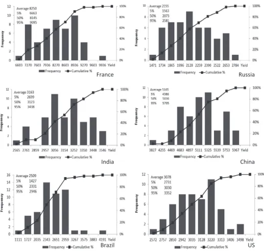
shocks according to different regions and crops. The analysis follows the approach used in Beach et al. (2010). The data have been detrended and normalised by 2012 yield. As an example, histograms (i.e. empirical probability distributions) of wheat yield based on a 52-year data series are depicted in Figure 1 for selected countries.
Yield distributions are characterised by multimodal shapes which precludes the use of mean-variance criteria and indicators (Markowitz, 1952). Figure 1 also shows the main statistics (i.e. average and main–5th, 50th and 95th–percentiles) of yield distributions. Countries such as France and China are characterised by higher yields and smaller yield variability. In Russia, US and Brazil, the yields are smaller and the variability is larger.
4.2. Robust solutions: Strategic and operational decisions
In this paper, robust solutions of stochastic GLOBIOM comprise strategic decisions (land allocation by LUS and storage capacities) and related adaptive decisions (trade,
France Russia
China India
Brazil US
Figure 1. Empirical wheat yield distribution by selected grain producers, 1960–2012
Notes:Horizontal axis denotes yield (in kilograms per hectare of harvested land) and vertical axis shows the number of years (frequency) the corresponding yield occurred in the 1960–2012
period. Cumulative distribution refers to the percentage of total of the yield occurrences at or below the value on the horizontal axis.
storage withdrawals, prices, demands). Stochastic GLOBIOM runs for a time horizon of 40 years (from 2010 to 2050) with a time step of 10 years. Stochastic yields are rep-resented by a finite set of historical yield scenarios from 1960 to 2015, analysed in sec-tion 4.1. In the calculasec-tions, we use food, feed, water, environmental and biofuel security constraints by requiring that, in each yield scenario, the demand for food, feeds and biofuels is not less than the exogenously given targeted levels, as in equa-tion (13) and funcequa-tions (14). Water security is introduced through a constraint on the total admissible water consumption by the following activities: crop production and processing, animal farming, forest production and processing, and biofuel production and conversion. GHG emissions targets from LUS (Valinet al., 2013) are included as environmental security constraints.
The benefits of robust solutions derived with stochastic GLOBIOM over the solu-tions of its deterministic counterpart are measured with the VSS. The VSS is calcu-lated by comparing the value of the stochastic goal functionF(x*sto) (equation S1 in the supplementary Appendix, available online) using the robust x*sto solution with the value of the stochastic goal functionF(x*det) using the deterministicx*detsolution. The value F(x*sto) is by about 25% higher than F(x*det), indicating the gains from using the stochastic model.
We analyse two cases of policy recommendations. The first case (C1) represents a popular approach to examining uncertainty and risks through a scenario analysis; that is, deterministic GLOBIOM is run in a ‘what-if’ manner, using alternative yield scenarios. In each scenario, the model provides scenario-specific recommendations. The second case (C2) involves stochastic GLOBIOM and corresponds to planning under uncertainty and risk when strategic (ex-ante) decisions on land allocation between LUS are made before information on stochastic yields becomes available. These decisions are adjusted using adaptive (ex-post) decisions (trade, storage with-drawals, prices) after the actual yield is observed, thus ensuring robustness of coordi-nated strategic and adaptive decisions. The combination of the decisions minimises the costs of implementing the strategic decisions and the costs of adjustment actions in response to each yield shock propagating through LUS.
In case (C1), GLOBIOM assumes that a spatio-temporal yield scenario occurs with probability 1, and there is no need to adjust to shocks. When all is known in advance, LUS can manage withoutex-post responses. In each yield shock scenario, the global commodity market redistributes production ‘shortages’ between regions so that food, energy, water and environmental constraints are satisfied. However, the implementa-tion of these scenario-dependent soluimplementa-tions can require considerable adjustments, such as conversion of forest into crop land or additional irrigation capacities if, for exam-ple, a drier than anticipated year occurs. Figure 2 presents percentage of land in dif-ferent LUS in C1 and C2 cases at the global level.
To fulfill FEWES targets in the face of all yield shocks, stochastic GLOBIOM sug-gests that crop land be used only 0.1% more compared with the results of determinis-tic GLOBIOM (C1) under the average yield scenario (Figure 2, panel a). In some yield scenarios, for example, those in the year 2000 when droughts occurred simulta-neously in Australia, Russia and China (Zou et al., 2005; Spinoni et al., 2015), the actual demand for crop land may exceed the robust requirement (demand) for crop land calculated using stochastic GLOBIOM.
Having the possibility of flexible ex-post adjustments to all potential scenarios, stochastic GLOBIOM recommends qualitatively different solutions. For example, natural ecosystems should be preserved, the conversion of natural forests into
managed woodland should slow down, grass land should be protected as an impor-tant feed source for livestock (see panels b and c in Figure 2). At the same time, it cal-culates a higher percentage of short-rotation tree plantations to fulfill bioenergy goals (Figure 2, panel e). All conversions come primarily from natural land (Figure 2, panel f). It is critically important that robust strategic decisions on land allocation among LUS are supplemented with adaptive scenario-specific trade decisionsysin the objec-tive function (12). Stochastic GLOBIOM accounts for spatial dependencies between yield shocks (FAO, 2011) and suggests scenario-specific geographical diversification of trade across uncorrelated (or negatively correlated) regions and commodities.
(a)Crop land (b)Grass land
(c)Natural forest (d)Managed forest
Planted forest Natural land
9.0 9.5 10.0 10.5 11.0 11.5 12.0 12.5 2010 2020 2030 2040 2050
Robust, C2 Average yield scenario, C1 2000 yield shock scenario, C1 17 18 19 20 21 22 23 24 2010 2020 2030 2040 2050
Robust, C2 Average yield scenario, C1 2000 yield shock scenario, C1
0 5 10 15 20 25 30 35 40 2010 2020 2030 2040 2050
Robust, C2 Average yield scenario, C1 2000 yield shock scenario, C1
0 2 4 6 8 10 12 2010 2020 2030 2040 2050
Robust, C2 Average yield scenario, C1 2000 yield shock scenario, C1
0.0 0.2 0.4 0.6 0.8 1.0 2010 2020 2030 2040 2050
Robust, C2 Average yield scenario, C1 2000 yield shock scenario, C1 23 24 25 26 27 28 29 2010 2020 2030 2040 2050
Robust, C2 Average yield scenario, C1 2000 yield shock scenario, C1
(e) (f)
Figure 2. Percentage of total land occupied by different LUS calculated using stochastic GLO-BIOM (Robust, C2), deterministic GLOGLO-BIOM under the average yield scenario (Average yield scenario, C1), and deterministic GLOBIOM under extreme shock scenario (2000 yield shock
scenario, C1). Horizontal axis labels simulation year and vertical axis identifies percent. (a) Crop land; (b) Grass land; (c) Natural forest; (d) Managed forest; (e) Planted forest; (f) Natural
To hedge global systemic risks and ensure FEWES goals, stochastic GLOBIOM makes use of storage facilities (which in the deterministic case are not required) to hedge regional and global (systemic) risks of shortfalls. They are essential for self-suf-ficient management of interdependent systemic risks to cover food demand when trad-ing is restricted or limited because of a direct or indirect (induced) yield and price shocks, or when land and water resources are scarce. Thus, storage can be viewed as insurance in cases where no other sources of supply, domestic or foreign, are avail-able. In this sense, storage capacities measure the systemic risks and (in)security, as discussed in section 3.3. From the formal point of view, storage withdrawals corre-spond to decision variables zisin (12) and (21). By changing pi, the stochastic model can achieve more or less systemic risk hedging. Adjustments of storage can be intro-duced to help ensure the required global FEWES levels, as discussed in section 3.3, equation (21).
Our calculations using stochastic GLOBIOM show that stochastic yields induce considerable volatility of global prices affecting various regions (Wright, 2011). This reduces the robustness of trade-based systemic risk management. Therefore, robust solutions of stochastic GLOBIOM in the presence of grain storage can increase the feasibility of biofuel targets, as discussed in section 2.2. For example, storage capacities (Figure 3) of about 80 and 300 thousand tons for rape and sun-flower, respectively, modulate the instantaneous demand for crop land caused by a yield shock (similar to the year 2000, as in Figure 2, panel a), and decrease the investments in and conversion of rainfed land into irrigated land to sustain rare high-impact shocks. Global reserves (Figure 3) of about 1,000, 250, 80 and 300 thousand tons of rice, barley, wheat, rape, sunflower, respectively, can obviate the need for investment in the irrigation of about 3,545 thousand hectares of agricul-tural land globally.
The availability of storage decreases prices and stimulates the increase in demand for commodities produced in interdependent LUS and necessary for FEWES. Fig-ure 4 compares global demand for selected crops. For example, stochastic GLO-BIOM allows that rice and wheat demand be increased by about 4.5% and 6%, respectively, compared with the deterministic model. On the other hand, the model suggests that production of rape and sunflower be decreased by about 5% and 6%, respectively. Stochastic GLOBIOM also recommends that biofuel targets can be ful-filled at lower cost through using cheaper biofuel feedstocks, e.g. second-generation biofuels from lignocellulosic biomass produced on short rotation tree plantations (Figure 1, panel e).
5. Concluding Remarks
The paper develops the stochastic GLOBIOM model, accounting for interdependen-cies among the main LUS on the global, national, and grid-cell levels. As section 2 demonstrates, shocks due, for example, to weather variability, may induce systemic risks that implicitly affect non- risky regions and activities. Analysis of FEWES in LUS under these ‘distributed’ risks requires robust solutions that comprise a proper set of ex-ante strategic (first-stage) and ex-post adaptive (second-stage) decisions enabling flexible adjustments to be made when new information becomes available. Thus, the ex-ante first-stage decisions cover only a fraction (quantile) of the risks determined by the FEWES requirement, whereas second-stage decisions hedge the rest of the exposure.
The risks in general stochastic GLOBIOM are defined by a system of quantile-based multi-dimensional security equations characterising production and resource shortfalls (shortages) at regional and global level (section 3). Robust management of shortfalls requires additional decisions to be made, for example, such as grain, water and energy stores, where storage capacities are similar to global and regional catastro-phe funds. In section 4 we show that stochastic GLOBIOM calculates robust grain and oilseed storage, which, in the presence of yield shocks and resource constraints help to fulfill combined FEWES targets (e.g. biofuel security) at lower costs without diverting grains from human consumption. By proper risk-adjusted spatial redistribu-tion of producredistribu-tion and selecredistribu-tion of management strategies and processing technolo-gies, stochastic GLOBIOM suggests lowering production of biofuel crops such as rape and sunflower and instead making use of cheaper feedstocks such as lignocellu-losic biomass from short rotation tree plantations. Analysing grain and oilseed stor-age is essential for self-sufficiency of world regions coping with potentially extreme events affecting large territories; for example, droughts may reduce yields, restrict trading, increase prices, and so on.
The combination of robustex-anteandex-postsolutions is evaluated by stochastic GLOBIOM for 28 world regions accounting for interdependent trade and respecting security constraints. We find that, in many regions, current policies relying on degen-erated solutions from deterministic models are not robust. The results of stochastic and deterministic GLOBIOM are compared at the global level showing that while the
(a) Rice. (b) Wheat.
(c) Rape. (d) Sunflower. 0% 20% 40% 60% 80% 100% 0 5 10 15 20 25 30 140 304 469 633 798 962 1126 1291 1455 1620 188 0 Frequency Frequency Cumulative % 0% 20% 40% 60% 80% 100% 0 2 4 6 8 10 12 14 16 18 194 198 203 207 212 216 221 225 229 234 239 Frequency Frequency Cumulative % 0% 20% 40% 60% 80% 100% 0 2 4 6 8 10 12 14 16 18 9 16 24 32 40 48 56 64 71 79 87 Frequency Frequency Cumulative % 0% 20% 40% 60% 80% 100% 0 5 10 15 20 25 30 35 44 177 309 442 575 707 840 972 1105 1238 1370 Frequency Frequency Cumulative %
Figure 3. Distribution of storage withdrawals, in thousand tons, at the global level. Frequency refers to the absolute number of withdrawals within a range identified on the horizontal axis. Cumulative refers to the percentage of total withdrawals at or below the value on the horizontal
robust land allocation among LUS fulfills FEWES targets in the face of all yield shocks, the policy recommendations from deterministic GLOBIOM are scenario-dependent. For example, in some scenarios the demand for crop land may exceed the robust requirement (demand) calculated using stochastic GLOBIOM. In section 4, the benefits of robust solutions derived with stochastic GLOBIOM over the solutions derived by scenario analysis of its deterministic counterpart are measured with the VSS. The calculated VSS indicates the importance of including uncertainties when designing robust solutions.
Supporting Information
Additional Supporting Information may be found in the online version of this article: Appendix S1.Detailed description of stochastic GLOBIOM.
References
Agarwal, C., Green, G., Grove, J., Evans, T. and Schweik, C.A Review and Assessment of Land-Use Change Models: Dynamics of Space, Time, and Human Choice, USDA Forest Ser-vice General Report No. NE-297, 2002.
Arrow, K. J. and Fisher, A. C. ‘Preservation, uncertainty and irreversibility’,Quarterly Journal of Economics, Vol. 88, (1974) pp. 312–319.
Beach, R., Zhen, C., Rejesus, R., Sinha, P., Lentz, A., Vedenov, D. and McCarl, B.Climate Change Impacts On Crop Insurance, RTI-USDA Risk Management Agency Report Number No. 0211911, 2010.
(a)Rice (b) Wheat
(c)Rape. (d) Sunflower. 0 200 400 600 800 1000 2000 2010 2020 2030 2040 2050
Average yield scenario, C1 Robust, C2
0 100 200 300 400 500 600 700 2000 2010 2020 2030 2040 2050
Average yield scenario, C1 Robust, C2
0 5 10 15 20 25 30 2000 2010 2020 2030 2040 2050
Average yield scenario, C1 Robust, C2
0 2 4 6 8 10 12 14 2000 2010 2020 2030 2040 2050
Average yield scenario, C1 Robust, C2
Figure 4. Global demand for selected agricultural commodities calculated using deterministic GLOBIOM under the average yield scenario (Average yield scenario, C1); using stochastic GLOBIOM (Robust, C2). Horizontal axis identifies simulation years and vertical axis shows
Birge, J. R. ‘The value of the stochastic solution in stochastic linear programs with fixed recourse’,Mathematical Programming, Vol. 24, (1982) pp. 314–325.
Birge, J. R. and Louveaux, F. Introduction to Stochastic Programming (New York, NY: Springer Verlag, 1997).
Colin, C. and Kunreuther, H. ‘Making Decisions about Liability and Insurance: Editors Com-ments’,Journal of Risk and Uncertainty, Vol. 7, (1993) pp. 5–15.
Coyle, W. ‘The future of biofuels: A global perspective’, Amber Waves (ERS Publication), Vol. 5, (2007) pp. 24–29.
Deaton, A. and Laroque, G. ‘Competitive storage and commodity price dynamics’,Journal of Political Economy, Vol. 104, (1996) pp. 896–923.
Ermoliev, Y. and Hordijk, L. ‘Global changes: Facets of robust decisions’, in: K. Marti, Y. Ermoliev, M. Makowski and G. Pflug (eds.),Coping with Uncertainty: Modeling and Policy Issue(Berlin, Germany: Springer Verlag, 2003).
Ermoliev, Y. and Jastremski, A.Stochastic Models in Economics(Moscow, Russia: Nauka, 1979). Ermoliev, Y. and Norkin, V. ‘On nonsmooth and discontinuous problems of stochastic systems
optimization’,European Journal of Operational Research, Vol. 101, (1997) pp. 230–244. Ermoliev, Y. and von Winterfeldt, D. ‘Systemic risk and security management’, in: Y. Ermoliev,
M. Makowski and K. Marti (eds.), Managing Safety of Heterogeneous Systems: Lecture Notes in Economics and Mathematical Systems (Berlin, Heidelberg, Germany: Springer Verlag, 2012, pp. 19–49.
Ermoliev, Y. and Wets, R. J.-B.Numerical Techniques for Stochastic Optimization(Heidelberg, Germany: Springer Verlag, 1988).
Ermoliev, Y., Ermolieva, T., MacDonald, G. and Norkin, V. ‘Stochastic optimization of insur-ance portfolios for managing exposure to catastrophic risks’,Annals of Operations Research, Vol. 99, (2000a) pp. 207–225.
Ermoliev, Y., Ermolieva, T., MacDonald, G. and Norkin, V. ‘Insurability of catastrophic risks: The stochastic optimization model’,Optimization, Vol. 47, (2000b) pp. 251–265.
FAO.The State of Food Insecurity in the World, Report of Food and Agriculture Organization of the United Nations, Rome, 2009.
FAO.The State of the World’s Land and Water Resources for Food and Agriculture (SOLAW)
–Managing Systems at Risk, Report of Food and Agriculture Organization of the United Nations, Rome, 2011.
FAO, IFAD, IMF, OECD, UNCTAD, WFP, the World Bank, the WTO, IFPRI, UNHLTF. Price Volatility in Food and Agricultural Markets: Policy Responses, Policy Report, 2011. Avail-able at: http://www.oecd.org/tad/agricultural-trade/48152638.pdf (last accessed 20.08.2015). GFDRR.Managing Disaster Risks for a Resilient Future: A Work Plan for the Global Facility
for Disaster Reduction and Recovery, 2016–2018 (Washington, DC: World Bank Global Facility for Disaster Reduction and Recovery (GFDRR), 2015).
Gielen, D. J., Gerlagh, T. and Bos, A. J. M.MATTER 1.0–A MARKAL Energy and Materials System – Model Characterisation, ECN Report No. ECN-C-98-085 (ECN, Petten, the Netherlands, 1998).
Gielen, D. J., Bos, A. J. M., deFeber, M. A. P. C. and Gerlagh, T.Biomass for Greenhouse Gas Emission Reduction Task 8: Optimal Emission Reduction Strategiesfor Western Europe, ECN Report No. ECN-C-00-001 (ECN, Petten, the Netherlands, 2000).
Grain. Against the Grain: Land grabbing for biofuels must stop, Grain Report, 2013. Available at: http://www.grain.org/article/entries/4653-land-grabbing-for-biofuels-must-stop (last accessed 05.04.2015).
Gustafson, R. L. ‘Implications of recent research on optimal storage rules’, Journal of Farm Economics, Vol. 38, (1958) pp. 290–300.
Havlık, P., Schneider, U. A., Schmid, E., Boettcher, H., Fritz, S., Skalsky, R., Aoki, K., de Cara, S., Kindermann, G., Kraxner, F., Leduc, S., McCallum, I., Mosnier, A., Sauer, T. and Obersteiner, M. ‘Global land-use implications of first and second generation biofuel targets’, Energy Policy, Vol. 39, (2011) pp. 5690–5702.
Headey, D.Rethinking the Global Food Crisis: The Role of Trade Shocks, Discussion Paper No. 00958 (IFPRI, 2010). Available at: http://www.ifpri.org/sites/default/files/publications/ ifpridp00958.pdf (last accessed 05.04.2015).
James, W. P. T. and Schofield, E. C.Human Energy Requirements: A Manual for Planners and Nutritionists(Oxford, UK: Oxford Medical Publications under arrangement with FAO, 1990). Kall, P. and Mayer, J.Stochastic Linear Programming: Models, Theory, and Computation(New
York, NY: Springer-Verlag, 2004).
Kok, K. and Winograd, M. ‘Modeling land-use change for Central America, with reference to the impact of Hurricane Mitch’,Ecological Modelling, Vol. 149, (2002) pp. 53–69.
Leclere, D., Havlık, P., Fuss, S., Schmid, E., Mosnier, A., Walsh, B., Valin, H., Herrero, M., Khabarov, N. and Obersteiner, M. ‘Climate change induced transformations of agricultural systems: Insights from a global model’, Environmental Research Letters, Vol. 9, (2014) pp. 124018.
Liu, J., Williams, J. R., Zehnder, A. J. and Yang, H. ‘GEPIC–modelling wheat yield and crop water productivity with high resolution on a global scale’, Agricultural Systems, Vol. 94, (2007) pp. 478–493.
Markowitz, H. M. ‘Portfolio selection’,The Journal of Finance, Vol. 7, (1952) pp. 77–91. Marti, K.Stochastic optimization methods(Heidelberg, Germany: Springer Verlag, 2008). McCarl, B. A. and Schneider, U. ‘U.S. agriculture’s role in a greenhouse gas mitigation world:
An economic perspective’,Review of Agricultural Economics, Vol. 22, (2000) pp. 134–159. Myers, N. ‘Environment and security’,Foreign Policy, Vol. 74, (1989) pp. 23–41.
OECD.Emerging Risks in the 21stCentury: An Agenda for Action(Paris, France: OECD Publi-cation Service, 2003).
Prekopa, A. ‘Numerical solution of probabilistic constrained programming problems’, in Y. Ermoliev and R. J.-B. Wets (eds.),Numerical Techniques for Stochastic Optimization(New York, NY: Springer Verlag, 1988, pp. 123–139).
Swiss Re.Partnering for Food Security In Emerging Markets(Einsiedeln, Germany: Sigma, EA Druck Verlag AG, 2013).
Rockafellar, R. T. and Uryasev, S. ‘Optimization of conditional value-at-risk’,Journal of Risk, Vol. 2, (2000) pp. 21–41.
Spinoni, J., Naumann, G., Vogt, J. and Barbosa, P. ‘The biggest drought events in Europe from 1950 to 2012’,Journal of Hydrology: Regional Studies, Vol. 3, (2015) pp. 509–524.
Stiglitz, J. E. ‘Incentives and risk sharing in sharecropping’, Review of Economic Studies, Vol. 41, (1974) pp. 219–255.
US Department of Energy.World Biofuels Production Potential: Understanding the Challenges To Meeting the U.S. Renewable Fuel Standard(Washington, DC: Office of Policy and Inter-national Affairs, 2008).
Valin, H., Havlik, P., Mosnier, A., Herrero, M., Schmid, E. and Obersteiner, M. ‘Agricultural productivity and greenhouse gas emissions: Trade-offs or synergies between mitigation and food security?’,Environmental Research Letters, Vol. 8, (2013) pp. 035019.
Veldkamp, A. and Fresco, L. ‘CLUE-CR: An integrated multi-scale model to simulate land use change scenarios in Costa Rica’,Ecological Modelling, Vol. 91, (1996) pp. 231–248.
Verburg, P., Chen, Y. and Veldkamp, A. ‘Spatial explorations of land-use change and grain production in China’,Agriculture, Ecosystems and Environment, Vol. 82, (2000) pp. 333–354. WHO.Energy and Protein Requirements, Report of a joint FAO/WHO/UNU expert
consulta-tion, WHO Technical Report Series No. 724, 1985. Available at: http://www.fao.org/ doCReP/003/aa040e/AA040E00.htm (last accessed 30.05.2015).
Wright, B. ‘The economics of grain price volatility’,Applied Economic Perspectives and Policy, Vol. 33, (2011) pp. 32–58.
Zou, X., Zhai, P. and Zhang, Q. ‘Variations in droughts over China: 1951–2003’,Geographical Research Letters, Vol. 32, (2005) p. L04707.