University of South Florida
Scholar Commons
Graduate Theses and Dissertations Graduate School
3-27-2015
The Impact of Bus Rapid Transit Implementation
on Residential Property Values: A Case Study in
Reno, NV
Steven Thomas Ulloa
University of South Florida, [email protected]
Follow this and additional works at:https://scholarcommons.usf.edu/etd
Part of theGeography Commons
This Thesis is brought to you for free and open access by the Graduate School at Scholar Commons. It has been accepted for inclusion in Graduate Theses and Dissertations by an authorized administrator of Scholar Commons. For more information, please [email protected].
Scholar Commons Citation
Ulloa, Steven Thomas, "The Impact of Bus Rapid Transit Implementation on Residential Property Values: A Case Study in Reno, NV" (2015).Graduate Theses and Dissertations.
The Impact of Bus Rapid Transit Implementation on Residential Property Values: A Case Study in Reno, Nevada
by
Steven Thomas Ulloa
A thesis submitted in partial fulfillment of the requirements for the degree of
Master of Arts School of Geosciences College of Arts and Sciences
University of South Florida
Major Professor: Steven Reader, Ph.D. Joni Downs, Ph.D.
Ruiliang Pu, Ph.D.
Date of Approval: March 27, 2015
Dedication
I dedicate this research to my mother, Olinda and my grandmother Ana who passed away while completing this work. Their unwavering guidance and encouragement has allowed me to pursue my dreams and goals.
I also dedicate this research to my father, Rafael and sisters, Jislayne and Mayrene for keeping me grounded and laughing throughout this process.
I dedicate this work to my partner, Derek. I am sincerely appreciative of his support and encouragement throughout this research.
Acknowledgments
I would like to thank Dr. Steven Reader for his guidance and mentorship not only on this research but throughout most of my undergraduate and graduate education at the University of South Florida. I am truly grateful to have had a thoughtful professor who truly cares about the success of his students. I would also like to thank Dr. Joni Downs and Dr. Ruiliang Pu for participating on my thesis committee and for their assistance in making this research
successful. Finally, I thank the team at the Washoe County Property Appraiser’s Office for their help in providing the necessary data to make this research possible.
Table of Contents
Table of Contents ... i
List of Tables ... iii
List of Figures ... iv
Abstract ...1
Chapter One: Background ...2
Bus Rapid Transit ...2
Real Estate Market Fluctuations of the 2000s ...3
Chapter Two: Literature Review ...5
Innovation and Significance of this Research ...8
Research Question...9
Chapter Three: Case Study ...12
Reno, NV ...12
RTC Rapid ...14
Chapter Four: Data ...18
Property Data ...18
Property Characteristics ...21
Sales Price Adjustment ...23
Socio-Demographic and Neighborhood Data ...26
Time Periods ...28
Distance Data ...30
Chapter Five: Methodology ...32
Descriptive Data Analysis ...32
Hedonic Price Method ...33
Modeling ...34
Chapter Six: Results & Discussion ...37
Descriptive Data Analysis ...37
Hedonic Price Regressions ...62
Chapter Seven: Conclusions & Limitations ...79
References ...82
Appendix A: Land Use Codes ...86
List of Tables
Table 2-1. Literature Review...10
Table 3-1. Demographics of Reno, NV ...13
Table 3-2. Descriptive Statistics of Residential Properties in Reno, NV ...14
Table 3-3. RTC Service Description ...16
Table 3-4. RTC Implementation Timeline ...16
Table 4-1. Property Data Description...20
Table 4-2. Descriptive Statistics of Properties Sold in Study Area...21
Table 4-3. Descriptive Statistics of Properties Sold in Study Area, Continued ...21
Table 4-4. Median Unadjusted & Adjusted Sales Price ...24
Table 4-5. Socio-Demographic/Neighborhood Data Description ...27
Table 4-6. Socio-Demographic/Neighborhood Descriptive Statistics...28
Table 4-7. Time Period of Important BRT/Real Estate Market Events ...29
Table 4-8. Distance Data Descriptive Statistics ...31
Table 5-1. Variable Descriptive Statistics ...32
Table 5-2. Variable Descriptive Statistics, Continued ...33
Table 5-3: Hedonic Price Models ...35
List of Figures
Figure 3.1. RTC Service Map ...15
Figure 3.2. RTC Rapid Vehicle (Photo Credit: Steven Ulloa) ...17
Figure 3.3. RTC Rapid Station (Photo Credit: Steven Ulloa) ...17
Figure 4.1. Sales Count by Year Histogram ...22
Figure 4.2. Adjusted Sales Price Map ...25
Figure 4.3. Sales Price (Unadjusted & Adjusted) of Properties Sold in Study Area ...26
Figure 4.4. Sales Price (Unadjusted) of Properties Sold in Study Area with Periods ...29
Figure 4.5. Period Histogram ...30
Figure 6.1. Adjusted Sales Price Non-Transformed Histogram ...37
Figure 6.2. Adjusted Sales Price Transformed Histogram ...38
Figure 6.3. BldgSF Non-Transformed Histogram ...39
Figure 6.4. Log(BldgSF) Histogram ...39
Figure 6.5. Log(BldgSF) Scatterplot ...40
Figure 6.6. Beds Histogram ...40
Figure 6.7. Beds Scatterplot ...41
Figure 6.8. Baths Histogram ...42
Figure 6.12. Building Type Histogram ...44
Figure 6.13. Building Type Boxplot ...45
Figure 6.14. Garage Histogram ...45
Figure 6.15. Garage Scatterplot ...46
Figure 6.16. Basement Histogram...47
Figure 6.17. Basement Scatterplot ...47
Figure 6.18. Age Non-Transformed Histogram...48
Figure 6.19. Age2 Histogram ...48
Figure 6.20. Age2 Scatterplot ...49
Figure 6.21. MINC Non-Transformed Histogram ...50
Figure 6.22. MINC2 Histogram ...50
Figure 6.23. MINC Map ...51
Figure 6.24. MINC2 Scatterplot ...52
Figure 6.25. PNOVEH Histogram ...53
Figure 6.26. PNOVEH Scatterplot...53
Figure 6.27. PNOVEH Map ...54
Figure 6.28. PNWHITE Histogram ...55
Figure 6.29. PNWHITE Scatterplot ...56
Figure 6.30. PNWHITE Map ...57
Figure 6.31. PRENTHistogram ...58
Figure 6.32. PRENT2 Histogram ...59
Figure 6.34. PRENT Map ...60
Figure 6.35. Distance Histogram ...61
Figure 6.36. Distance Scatterplot ...62
Figure 6.37. Log(BldgSF) Effect Plot ...67
Figure 6.38. Beds Effect Plot ...67
Figure 6.39. Baths Effect Plot ...68
Figure 6.40. Half Baths Effect Plot ...69
Figure 6.41. Building Type Effect Plot ...69
Figure 6.42. Basement Effect Plot ...70
Figure 6.43. Age2 Effect Plot ...71
Figure 6.44. MINC2 Effect Plot ...71
Figure 6.45. PNOVEH Effect Plot ...72
Figure 6.46. PNWHITE Effect Plot ...73
Figure 6.47. PNRENT2 Effect Plot ...74
Figure 6.48. Distance Effect Plot (Model 1) ...75
Figure 6.49. Distance Effect Plot (Model 2) ...75
Figure 6.50. Distance and Period Interaction Effect Plot (Model 3) ...77
Abstract
Since literature that evaluates the impacts that Bus Rapid Transit (BRT) has on surrounding property values is limited, this research contributes to this research by investigating if proximity to a BRT station has an effect, either positive or negative, on
residential housing values. Further, it investigates if the nature and extent of this effect varied during different stages of implementation of the BRT system and different housing market conditions. Fluctuations in sale prices were mitigated based on a six month moving median. Four hedonic price models were then used to evaluate the influence of independent variables on the dependent variable, adjusted sales price. Results indicated that properties that were in an area between 0.4 and 0.8 mile (network distance) away from a BRT station, possessed about a $5,000 premium in sales price during the bust and initial recovery of the real estate market that occurred between 2009 and 2013. Additional results also indicated that in areas where the percentage of households without access to a vehicle increased, sales prices on residential properties also increased. This study did not employ the use of spatial models and concludes that such models should be used in future research to account for spatial autocorrelation. Further, this research suggests that additional geographic variables should be used to evaluate how residents value accessibility to other transportation systems when compared to BRT.
Chapter One: Background
Bus Rapid Transit
A BRT system is a rapid mode of public transportation that uses a rubber-tired vehicle to transport passengers from one station to another through a network of bus lanes that make up a system utilizing technologies such as: dedicated running ways, uniquely designed bus stations, improved fare collection, and distinctive system branding. Advanced BRT systems possess features such as: Intelligent Transportation Systems (ITS), queue jumps, electric/hybrid vehicles, and high-frequency service (American Public Transportation Association, 2013)
Constructed to mimic the performance and dependability of light rail systems, BRT is less expensive and easier to implement. BRT systems are often converted to light-rail or streetcar lines once passenger thresholds are met (Levinson et al., 2003). The average capital cost per mile for BRT is $13.5 million. In comparison, the capital cost per mile for light rail is $34.8 million. The cost of constructing BRT depends on the location of the bus route, right-of-ways, construction of station structures, placement of park-and-ride facilities, and other
relevant technologies that are included in the system (United States General Accounting Office, 2011).
The first BRT system began operation in Curitiba, Brazil in 1974. Regarded as an
2006, the system served over 1.4 million passengers (Cain et al., 2006). In 2012, the system served over 2.2 million passengers (Duarate et al., 2012)
The successful use of BRT in South America has spurred interest in developing this type of mass transportation in the United States. Chicago became the first United States city to implement BRT technologies within its existing transportation system in 1939. Pittsburgh opened a complete BRT system in 1983 and is now widely considered to have one of the most successful busways in the United States (Perk & Catalá, 2009). Other notable American BRT projects include an 11-mile busway in El Monte, a suburb of Los Angeles, which opened in 1973, and a BRT system in Washington, DC (Levinson et al., 2003). Although it is less popular than other transport systems, BRT is slowly gaining interest in the United States. In 2012, there were 66 BRT bus routes operating in the United States (National Bus Rapid Transit Institute, 2012). As of 2013, there are 130 BRT systems worldwide (Suzuki, 2013).
Real Estate Market Fluctuations of the 2000s
Local municipalities, more than ever, are enhancing transportation systems as a means to encourage development, spur commercial investment, and ameliorate citizens’ quality-of-life. However, the U.S. real estate financial downturn of the late 2000s crippled local
government budgets, making planning for transportation systems difficult. A housing bubble occurred causing housing prices in the United States to increase to unsustainable levels between 1997 and 2006 when the typical American home increased in value by 124 percent (The Economist, 2007). The market corrected itself in late 2006, and housing values rapidly retracted causing the housing bubble to “burst”. Homeowners that mortgaged their properties
at the height of the market, suddenly found themselves “underwater” or in negative equity on their properties. Credit conditions became difficult and many homeowners, unable to refinance variable interest rate mortgages, defaulted on loans. This caused the largest foreclosure
movement in American history. By the end of 2007, nearly 1.3 million properties and 13.8 percent of subprime mortgages were in the foreclosure process (RealtyTrac , 2008). By 2008, seventeen percent of subprime mortgages were in foreclosure (RealtyTrac, 2009). Also in the same year, nearly 2.3 million properties were in foreclosure (Immergluck, 2009).
The decline of the housing market caused severe consequences to the American economy. Families that were not able to afford their homes abandoned many suburban neighborhoods. By September 2008, housing prices fell by over 20 percent (The Economist, 2008). Investments made against real estate were lost causing individuals and commercial organizations to lose billions in savings. The loss in tax revenue also caused many municipalities around the country to lose millions in local budgets.
Chapter Two:Literature Review
Most studies found that property values near BRT stations were higher than those that were farther away. Perk & Catalá (2009) found an inverse relationship between distance to a BRT station and property values in Pittsburgh concluding that a residential property that was 1,000 feet away from a station was valued $9,475 less than a property that was 100 feet away from the station. Similarly, Perk et al., (2013) found that condominiums near the Silver Line BRT in Boston possessed a 7.6 percent premium on the mean sale price per square foot value as distance to the station decreased. Rodriguez & Targa (2007) found that for every five minutes closer to a BRT Station of the TransMilenio system in Bogotá there was between a 6.8 and 9.3 percent increase in asking rental price. When analyzing the same system, Munoz-Raskin (2011) found evidence that properties within a ten minute walk of a station experienced between a 2.2 and 2.9 percent increase in value.
Findings in the studies reviewed above are similar to results found in literature that evaluates other types of transportation systems. Gatzlaff & Smith (1993) did not find statistically significant results in initial analyses. However, their secondary models found that residential properties at higher price points, near MetroRail, the subway system in Miami, had a more significant increase in value than properties found in poorer neighborhoods. Baum-Snow & Kahn (2000) identified that decreasing distance from 3-kilometers to 1-kilometer to commuter rail/light rail stations of systems in Boston, Atlanta, Chicago, Portland, and Washington, DC, increased monthly rents by $19 and home values by $4,972. Chen et al., (1997) found that for each additional meter beyond
100 meters from a Portland MAX light rail station, a residential property value declined $32.20. Bowes & Inlanfeldt (2001) found that properties between one and three miles from a MARTA station, the subway in Atlanta, had higher values than those farther away. Garrett (2004) found that when distance decreased to a Metrolink station, the light rail system in St. Louis, home values increased an average $139.92 for every 10 feet closer to the station beyond 1,460 feet. Billings (2011) found that single-family homes, located 1-mile from a LYNX light rail station in Charlotte, had an aggregated benefit of $39.6 million while condominiums had an aggregated benefit of $57.6 million. Hess & Almeida (2007) found that properties were valued $2.31 (linear distance) and $0.99 (network distance) more for every foot closer to stations of Buffalo’s light rail system. It was found that properties that were 1,000 feet away from a station are worth between $990 and $2,310 more than the average home in the area. Brandt & Maennig (2011) found that for condominiums that were between 250 and 750 meters from a commuter rail station in Hamburg, there exists a premium of 4.6 percent in list price. Further, they found a EUR 4.2 million aggregated increase in property tax revenue for the local government. Haider & Miller (2007) found that residential properties that were near subway lines in Toronto, experienced a $4,000 increase in property value. McMillen & McDonald (2004) evaluated the impact that Chicago’s Midway Rapid Transit line had on residential property values during a 13 year period. Time graidents were constructed to evalute the impacts before construction of the line as well as three subsequent time points. It was found that immediately following the opening of the line there was a sharp decline in prices. The author concluded that this may be due to a correction in
This translated to an aggregated increase of $215.9 million or an average of about $6,000 per home. Efthymiou (2013) found that houses that were 500 meters from an Athens metro station possesed a higher purchase price ranging from 6.74 percent to 11.66 percent while rental prices in the same area possessed a premium of 4.2 percent to 6.21 percent. Concas (2013) conducted a study to determine how values of properties near limited access highways in Hillsborough County and Miami-Dade counties compared to controls groups. The author compared behaviors of the values before, during, and after construction of these limited access highway. Further, the author evaluates the “resilience” of these values during the U.S. real estate market decline in the late 2000s. The results of the analysis found minimal impacts on parcels in the treatment area during construction. However, parcels in the treatment area possessed a 3.4 to 7.3 percent premium in property value over parcels in the control area during the first year of operation. Five years following initial operation of the roadways, price premiums of between 4.6 and 5.2 percent were found in parcels in the treatment area.
There is evidence that being “too close” to a station does not increase value and can often decrease a property’s value. Bowes & Inlanfeldt (2001) found that the largest negative impacts to value were for properties within a zone located one-quarter mile away from a station. The authors attributed this to the externality effects of being too close to the system. Brandt & Maennig (2011) determined that properties within 250 meters from a station, did not have premiums significantly different from zero. Chen et al., (1997) found the largest benefits beyond 100 meters from a station. Perk & Catalá (2009) found that residential properties that were one-tenth of a mile from the BRT system in Pittsburgh valued $5,904 less than if they were located somewhere else.
Chen et al., (1997) conducted a literature review to identify exploratory variables that are important in influencing housing prices. The findings identified the following variables in four categories:
Physical Property Attributes (i.e.: house size, number of bedrooms, number of bathrooms, age),
Neighborhood Attributes (i.e.: median household income, occupation structure, white/minority ratio, school quality, crime rate),
Locational Attributes (i.e.: distance to central business districts, distance to employment centers), and
Fiscal and Economic Externalities (i.e.: property tax rate, public facilities, zoning, air quality, traffic)
Table 2-1 outlines the literature reviewed and includes the scope of the study, the location in which the study was conducted and key results.
Innovation and Significance of this Research
Unfortunately, the influence that BRT has on the surrounding property values has not been evaluated as extensively as other transportation systems. Rodriguez & Targa (2007) suggested that the lack of research is attributed to the lack of permanence of the BRT system. Decision-makers and planners therefore are skeptical of BRT’s ability to encourage neighboring land development. Paradoxically, this lack of current research is discouraging future research.
many parcels can be near transportation stations, households are likely to pay more to secure the parcels with the best accessibility to those stations (Alonso, 1964). If this theory is applied to BRT, then it is possible that households will also be willing to pay more for properties near BRT stations (Rodriguez & Targa, 2007). Therefore, this research will determine if properties that are closer to BRT stations have higher sales prices than those that are further away.
At present, there is also an absence of literature that evaluates the influence that accessibility to transportation stations has on property values during housing market fluctuations. If it is demonstrated that property sale prices near BRT stations remained
consistent during housing market fluctuations, homeowners may be more inclined to purchase properties near BRT. This helps foster walkable communities, strengthens the urban network, and gives confidence to local leaders to continue to construct BRT. Therefore, this research will evaluate the planning, construction, and subsequent operation of a BRT system and its
influence on property values concurrently during the time the United States experienced major fluctuations in the real estate market. In doing this, this research will determine if BRT systems are capable of dampening decreases in sales prices of properties near stations.
Research Question
This research will address the following research question:
Does proximity to a Bus Rapid Transit have an effect, positive or negative, on residential housing values and, if so, does the nature and extent of this effect vary during different stages of implementation of the BRT system and under different housing market conditions?
Table 2-1. Literature Review Author(s)
& Year
Transportation
Type Scope of Study Location Results
Baum-Snow & Kahn (2000) Heavy Rail, Light Rail
Identify extent commuters are willing to switch modes of transit if it made more accessible,
demographics that benefit the most from transit improvements and how those improvements affect property values Boston, Atlanta, Chicago, Portland, Washington, DC
Better access indicates more use of transit. Decreasing accessible distance from 3km to 1km increases use by 1.4 percent. Inverse
relationship between distance to station and property values. Decreasing distance from 3km to 1km increases monthly rents by $19 and home values by $4,972
Billings
(2011) Light Rail
Measure aggregated effects that proximity has on surrounding commercial and condominium values within one mile from station
Charlotte
There exists an aggregated benefit of $40 million for condominiums and $56 million for
commercial properties for a neighborhood benefit of $97 million.
Bowes & Ihlanfeldt (2001)
Heavy Rail
Investigate impacts that proximity to stations has on single family home values, crime, and retail
employment
Atlanta
A price model finds that properties that are between zero and one-quarter mile from station have a value that is 19 percent less than those that are between 1-3 mile from a station. Properties that are between 1-3 miles from a station have a significantly higher value than those that are further away. Crime and retail models found that stations have less crime and retail locations have a higher positive impact the closer they are to a station and the further away they are from the Central Business District (CBD)
Brandt & Maenning (2011)
Heavy Rail
Identify relationship that proximity to a station has on condominium list prices
Hamburg, Germany
Properties that are within a 250-750 meter radius from a station have a 4.6 percent premium in property values. Properties closer to station have an insignificant increase. Total gain in property value resulting from better access is EUR 2.33 billion. Additional annual revenue from increase in land taxes is EUR 4.20 million. Higher premiums are found in properties in higher income neighborhoods
Chen et
al., (1997) Light Rail
Evaluate the relationship between single family home values and distance to station. Utilize distance between property and station to measure accessibility. Utilize distance between property and rail line to measure negative
externalities
Portland
For each additional meter beyond 100 meters beyond a station, a property declines in value by $32. The effects of distance between a property and rail line are negligible and outweighed by the positive effects of distance between a property and station.
Concas (2013)
Limited Access Highways
Quasi-experimental regression model to determine impacts proximity to limited access highways has on residential sale prices. Uses a treatment and control experiment evaluating change of value before, during and after construction
Hillsborough County & Miami-Dade County, FL
Minimal impacts on parcels in treatment area during construction. Treatment area possesses a 3.4-7.3 percent premium over parcel in the control area during the first year of operation. Years following operation, price premiums of 4.6 and 5.2 percent are found in parcels in the treatment area.
Efthymiou
(2013) Heavy Rail
Evaluate relationship between home purchase price located in the study area
Athens
Houses that were 500 meters found a Athens metro station possesed a higher purchase price ranging from 6.74 percent to 11.66 percent while rental prices in the same area possessed a premium of 4.2 percent to 6.21 percent
Table 2.1. Literature Review Summary (Continued) Author(s)
& Year
Transportation
Type Scope of Study Location Results
Garrett
(2004) Light Rail
Evaluate the relationship that proximity to stations has on residential properties located within one mile
St. Louis
Home values increased on average by $139 for every 10 feet closer to station beyond 1,460 feet from a station. No significant relationship between distance to track and home values.
Gatzlaff & Smith (1993)
Heavy Rail
Evaluate behavior of residential property values before and after construction of transportation system
Miami
Initial results did not yield statistically significant results. Later models found residential properties at higher price points near stations experienced a higher value increase than those in poorer neighborhoods.
Haider & Miller (2013)
Subway
Spatial autoregressive model to determine how proximity to different amenities effect property values
Toronto
Properties that are close to subway lines experience a $4,000 increase in property value. The authors also find however that most significant determinates of housing values were income, number of bedrooms, number of bathrooms, and number of parking spaces.
Hess & Almeida (2007)
Light Rail
Evaluate the impact that proximity to a station has on residential property values within one-half mile of station
Two equations are used: one evaluates stations collectively the other evaluates stations independently
Buffalo
First model found that properties are valued $2.31 (linear distance) and $0.99 (network distance) more for every foot closer to a station. Properties that are 1,000 feet away from a station are worth between $990 and $2,310 more than the average home. Second model found that the greatest effects are realized in higher income neighborhoods.
Munoz-Raskin (2011)
BRT
Hedonic model to evaluate the impact that distance to BRT has on residential property values
Bogotá, Colombia
Properties within a ten minute walk from a station experience between a 2.2 and 2.9 percent increase in property value. McMillen
& McDonald (2004)
Heavy Rail
Eevaluate the impact that a Chicago’s Midway Rapid Transit line effected residential property values during a 13 year period.
Chicago
There exists a 6.89 percent increase in homes closer to stations. This translates to an aggregated increase of $215.9 million or an average of about $6,000 per home
Perk & Catalá (2009)
BRT
Investigate the impacts that proximity to BRT stations has on residential property values
Pittsburgh
Decreasing marginal effects were found. Moving from 101 feet to 100 feet increases property values $19. A property that is 1,000 feet away from a station is valued $9,475 less than a property that is 100 feet away from a station.
Perk et
al., (2013) BRT
Estimate the impact of access to BRT station on sale prices of
condominium units within a quarter-mile radius
Boston There exists a 7.6 percent premium on the sale price of condominium units closer to a station.
Rodriguez & Targa (2007)
BRT
Evaluate the impact that distance to the nearest station has on rental price demanded of properties within 1.5km of BRT station. Euclidean distance to BRT line measure negative effects
Bogotá, Colombia
Properties that are within a five minute walking distance to a station has between a 6.8 and 9.3 percent increase in rental price demanded.
Chapter Three: Case Study
Reno, NV
A BRT system, located in Reno, NV, was used as the case study for this analysis. Reno is located in the State of Nevada and is the county seat of Washoe County. The metropolitan statistical area (MSA) is called Reno-Sparks but is informally known as Truckee-Meadows. Reno is often referred to as “The Biggest Little City in the World” and is famous for its abundance of casinos. Incorporated on May 8, 1868 after the construction of a depot that would connect the region with the First Transcontinental Railroad, Reno was known for its gold and silver mining activities as well as subsistence farming in the fertile valley. This attracted farmers from California, Oregon, and Washington and increased the population in the region. Gambling became Reno’s largest economy in 1905 after its legalization in the state.
According to the 2010 United States Census, Reno had 225,221 residents. This is a 21 percent increase from the 2000 United States Census when Reno had about 185,000 residents. The median household income in $48,846 in 2010 and $40,535 in 2000. There were almost 90,924 households in Reno in 2010 and 75,737 in 2000. Population density also decreased in 2010 to 2,186.4 persons per square mile from 2,611.4 in 2000. The percent of households without vehicles was 6.27 percent in 2010 and 8.07 percent in 2000. Minority races had the highest racial increase in 2010. The average household size declined to 2.43 in 2010 from 3.06
Table 3-1. Demographics of Reno, NV
2000 2010
Population 185,480 225,221
Median Household Income $40,530 $48,846 Persons per Square Mile 2,611.4 2,186.4 Percent No-Vehicle Households 8.07% 6.27%
Total Households 75,737 90,924
Average Household Size 3.06 2.43
White 173,986 167,179
Black 2,271 6,429
Asian 9,555 14,232
Hispanic (Any Race) 34,616 54,640
During the decline of the real estate market in 2006, Reno experienced some of highest foreclosures rates in the country. In 2009, Reno had the 9th highest foreclosure rate in the country. At that time, 1 in 37 homes were in the foreclosure process- an 80 percent change from the 3rd quarter of 2008 when the city had the most foreclosures in the country (CNN Money, 2013). Although foreclosures in the United States declined slightly two years later, Reno was still experiencing high foreclosure rates. In 2010, there were 3,369 foreclosure fillings representing 1 in every 54 homes (MSN Real Estate, 2011).
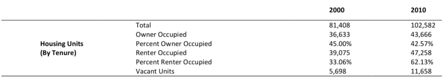
The average residential home sold between January 2002 and June 2013 had 3 bedrooms and 2 bathrooms. Further, the median property size during this time was about 1,760 square feet. The average home was built in 1978 and was about 27 years old. In 2000, Reno had a total of 81,408 housing units. This included 36,633 owner occupied units, 39,075 renter occupied units and 5,968 vacant units. In 2010, there were 102,582 housing units. This included 43,666 owner occupied units, 47,258 renter occupied units, and 11,658 vacant units (See Table 3-2).
Table 3-2. Descriptive Statistics of Residential Properties in Reno, NV 2000 2010 Housing Units (By Tenure) Total 81,408 102,582 Owner Occupied 36,633 43,666
Percent Owner Occupied 45.00% 42.57%
Renter Occupied 39,075 47,258
Percent Renter Occupied 33.06% 62.13%
Vacant Units 5,698 11,658
RTC Rapid
RTC Rapid is the BRT service of the Regional Transportation Commission of Washoe County (RTC), the legal organization responsible for providing and regulating transportation in the City of Reno and Washoe County. A study was conducted in 2003 to measure the feasibility and costs of converting a current RTC Bus Route (RTC Ride Route 1) into a BRT system (Meyer, Mohaddes Associates, Inc., 2003). The final proposal and funding for the BRT system in Reno was announced on October 29, 2004. A $7 million grant was awarded to RTC from the federal government to aid in financing the construction of two new transit centers and development of the rapid transit system along Virginia Street at an estimated cost of $34 million (EV World, 2004).
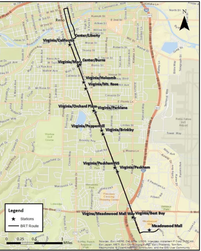
The first phase of the BRT system service launched on October 12, 2009. The route operated on Virginia Street between Downtown Reno in the north and the Meadowood Mall to the south. Initially, the system opened serving seven stops. Additional stops were added
incrementally. By December 2013, the system operated 15 stops. (See Figure 3.1 and Table 3-3. RTC Service Description). The service was federally funded for the first three years to
Table 3-3. RTC Service Description
Station Name Direction
Meadowood Mall Terminus/Commencement Virginia/Meadowood Mall Way Inbound
Virginia/Bestbuy Outbound Virginia/Peckham Inbound Virginia/Peckham NS Outbound Virginia/Brinkby Outbound Virginia/Peppermill Inbound Virginia/Parklane Inbound
Virginia/Orchard Plaza Outbound
Virginia/Holcomb Inbound
Virginia/Mt. Rose Outbound
Virginia/Mary Outbound
Virginia/Burns Inbound
Virginia/California Outbound
Center/Liberty Inbound
RTC Rapid is serviced by 60 foot articulated hybrid diesel/electric vehicles (White, 2013) (Figure 3.2). The adult fare is $2-the same fare for other transportation services in the RTC (Regional Transportation Commision, 2013). On October 19, 2009, RTC began designing new permanent RTC Stations as part of the next phase of the RTC system (Figure 3.3).
On May 15, 2012, RTC opened 14 new RTC Rapid stations, at the cost of about $6 million. These new stations possess covered waiting areas, expanded seating, next bus
information monitors, and ticket vending (Nelson, 2012). RTC also introduced two new transit stops on Center Street at Holcomb and Liberty Street (See Table 3-4).
Table 3-4. RTC Implementation Timeline
Date Event
Late 2003 Feasibility study for converting RTC Ride Route 1 into BRT completed October 29, 2004 Final Proposal and $7 million federal grant announced
October 12, 2009 Initial launch of ten stop BRT service
Figure 3.2. RTC Rapid Vehicle (Photo Credit: Steven Ulloa)
Chapter Four:Data
Literature reviewed indicates that a reasonable distance to access a public
transportation station is 0.25-0.50 mile. However, a study area of 1 mile network distance from each station of the BRT route in Reno was used to capture any effects that may exist beyond 0.50 mile. This research utilized four types of data:
1. Property data
2. Socio-Demographic/Neighborhood data 3. Distance data
4. Time
Property Data
Property data was obtained from the Washoe County Property Appraiser’s Office. Data received from the property appraiser was in the form of 12 tabular data files. Each file
contained information for any real estate sale transaction that took place between January 2002 and May 2013. Data within each file included: unique identifiers for a property, property address, sales date, sales price, year property was built, building type, property condition, construction type, presence of basement or garage, number of bedrooms, bathrooms, and half bathrooms, zoning types, land use codes, and transactions codes.
Washoe County Property Appraiser’s Office (Appendix A). Land use codes that identify residential properties were:
Code 12, Vacant Single Family Code 13, multi-residential Code 20, single family residence Code 21, condominium
Code 22-23, mobile home designation Code 25-34, multiple unit designations
Once residential sale transactions were identified, only those transactions that were representative of an actual sale and not a deed transfer, loan modification, or estate transfer were extracted. Using a chart located on the Washoe County Property Appraiser’s Office website, the following codes were used to exclude sales transactions from the dataset (Appendix B).
Code 1MGA Code 4MV Code 2MD
Next, those sales transactions that contained building types of only residential properties were extracted. This was completed by identifying those records that had the following the building types:
“APT RESIDENT and “Apt Res" “Duplex"
“SGL FAM RES" and "Sgl Fam Res" "TOWNHSE END" and "Townhse End" "TOWNHSE INS" and "Townhse Ins"
In order to achieve consistency in the building types within the dataset, building types were reclassified to the following categories:
“APT RESIDENT and “Apt Res" reclassified to “condo” “Duplex" remained the same
"HiRise Condo" reclassified to “condo”
“SGL FAM RES" and "Sgl Fam Res" reclassified to “single family” "TOWNHSE END" and "Townhse End" reclassified to “townhome” "TOWNHSE INS" and "Townhse Ins" reclassified to “townhome”
The files were joined to form a single dataset of residential property sale transactions in the study area. This file contained 4,304 records. Table 4-1 displays the property data that will be used in the analysis:
Table 4-1. Property Data Description
Source Description
Washoe County Property Appraiser
Sales Price
Number of bedrooms Number of bathrooms Number of half bathrooms Property Type
Square footage of property Garage
Basement
Property Characteristics
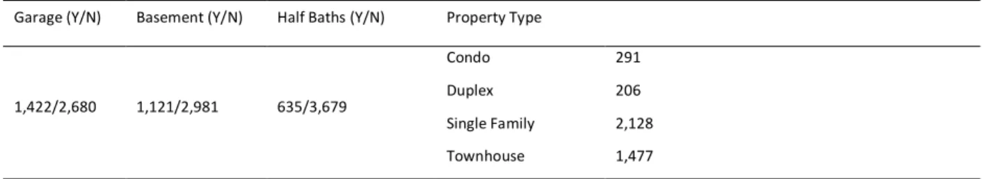
The average property sold within the study area during the 11 year span of the study was 45.46 years old, had 2 bedrooms, 1 full bathroom, 1 half bathroom, did not have a garage nor basement, and was a single family residence (See Table 4-2 and Table 4-3).
Table 4-2. Descriptive Statistics of Properties Sold in Study Area
Year Count of Sales Age in Years (Mean) Beds (Mean) Full Baths (Mean)
2002 473 43.28 2.47 1.48 2003 480 46.04 2.30 1.45 2004 577 45.39 2.20 1.41 2005 458 46.24 2.28 1.42 2006 324 45.30 2.21 1.41 2007 246 46.24 2.36 1.52 2008 202 41.60 2.42 1.60 2009 262 47.42 2.46 1.44 2010 348 46.88 2.20 1.42 2011 393 47.88 1.93 1.33 2012 403 44.16 1.97 1.44 2013 148 42.87 2.01 1.51 All Years 4,314 45.46 2.23 1.44
Table 4-3. Descriptive Statistics of Properties Sold in Study Area, Continued Garage (Y/N) Basement (Y/N) Half Baths (Y/N) Property Type
1,422/2,680 1,121/2,981 635/3,679
Condo 291 Duplex 206 Single Family 2,128 Townhouse 1,477
A closer look at the dataset revealed that several records contained anomalies in the number of bedrooms or bathrooms that a property contained. For example, a record displayed
that the property sold contained 8 bedrooms. Since the average property sold in the study area had only 2 bedrooms, this property contained a number of bedrooms that was extremely far from normal. After consulting with the property appraiser’s office website, it could not be determined that this property, or the other properties with similar anomalies, were errors. To account for these anomalies, any record that had more than 4 bedrooms was changed to 4 bedrooms. Similarly, any record that had more than 3 bathrooms was changed to 3 bathrooms. The fields that represented data for the presence of garage and basement were also changed to binary types where 1 indicated the presence of garage or basement and 0 represented the absence of garage or basement respectively.
During the 11 year time span, the amount of sales by year, in the study area, follows the fluctuations of the market (See Figure 4.1). The most sales occurred in 2004, with 577 sales and the fewest sales occurred in 2008 with only 202 sales within the study area.1
Figure 4.1. Sales Count by Year Histogram 0 100 200 300 400 500 600 700 2002 2003 2004 2005 2006 2007 2008 2009 2010 2011 2012 2013
Sales Price Adjustment
Data for this analysis spans an 11 year time period between 2002 and 2013. Recall in the earlier literature review that during this time period the real estate market experienced major fluctuations causing sales prices to change drastically. These fluctuations must be “taken out” of the sales prices in the dataset. The removal of these fluctuations ensured that any change that was found during modeling was due to the influence of the property characteristics, neighborhood and socio-demographic characteristics, distance, or time periods and not the exogenous factors of the real estate market fluctuations. The adjustment was first completed by obtaining a six month moving median for each transaction within the dataset. In other words, for each record, the median sales price of all properties sold 90 days before and 90 days after, was obtained. Once a six-month median for each transaction was obtained, a ratio was created which represented the relationship between that six-month median for each
transaction and the six month median sales price on April 1, 2002-which is $135,000. This date is selected because it represents the first date that a six-month moving median of each
transaction can be completed. The sales price adjustment is represented by the formula:
𝐴𝑆𝑃 = (𝐵𝐴𝑆𝐸
𝑆𝑀𝑀) ∗ 𝑃𝑟𝑖𝑐𝑒
Where, ASP= adjusted sales price for a given property; SMM= a six-month moving median sales price for any given property; Base= the six-month median sales price on April 1, 2002, and Price= the sales price for a given property on the date it was sold.
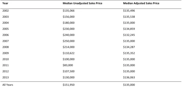
A map displays the adjusted sales price along the BRT route split up into 6 quantile classes. The highest adjusted sales prices are located northwest of the BRT route. The lowest adjusted sale prices are located northeast of the BRT route (See Figure 4.2). Table 4-4 and
Figure 4.3 display the un-adjusted and adjusted sales prices for properties within the study area.
Table 4-4. Median Unadjusted & Adjusted Sales Price
Year Median Unadjusted Sales Price Median Adjusted Sales Price
2002 $135,066 $135,496 2003 $156,000 $135,538 2004 $180,000 $135,000 2005 $230,000 $134,859 2006 $240,000 $132,245 2007 $250,000 $135,000 2008 $214,000 $134,287 2009 $110,622 $135,352 2010 $100,000 $135,000 2011 $83,000 $135,000 2012 $107,500 $135,000 2013 $130,000 $136,063 All Years $151,950 $135,000
Transactions that took place before April 1, 2002 and after February 22, 2013 are omitted from the dataset since it was not possible to create a six-month moving median for these records. The subsequent dataset had 4,112 records after these omissions.
Figure 4.3. Sales Price (Unadjusted & Adjusted) of Properties Sold in Study Area
Socio-Demographic and Neighborhood Data
This analysis used socio-demographic and neighborhood data that described the area that each property was located in as well as the socio-demographic makeup of the residents in the study area. The literature reviewed provides a framework for appropriate data types that should be used. Therefore, socio-demographic and neighborhood data that are commonly found in other studies, are used for this analysis (See Table 4-5). Data was obtained from the United States 2000 and 2010 censuses. The geography for the data was at the census tract level. There are 13 census tracts located within the study area.
Since socio-demographic and neighborhood data was only available for the years 2000 and 2010, data must be interpolated for the other years within the study’s time span. While
$135,066 $156,000 $180,000 $230,000 $240,000 $250,000 $214,000 $110,621 $100,000 $83,000 $107,500 $130,000 $135,496 $135,537 $135,000 $134,859 $132,244 $135,000 $134,286 $135,351 $135,000 $135,000 $135,000 $136,063 $0 $50,000 $100,000 $150,000 $200,000 $250,000 $300,000 2002 2003 2004 2005 2006 2007 2008 2009 2010 2011 2012 2013 Sal es P ri ce Sales Year
Table 4-5. Socio-Demographic/Neighborhood Data Description
Source Data Characteristic
United States Census (2010) 2010 American Community Survey 5-year Estimate & United States Census (2000) Summary File, Census Tract Level
Median household income
Percent of households without a vehicle Percent non-white
Percent of units that are renter occupied
Through the use of GIS software, the centroid for each property was identified. Next, the centroid was spatially joined to the 2000 census tract in which it intersects. Then the property centroid was intersected with the 2010 census tract. The spatial joins attached data from the 2000 and 2010 census to each property. Following the spatial joins, the data for the years 2001-2009 and 2011-2013 were interpolated. This was done by first obtaining a rate of change for median household income, percent of households without a vehicle, percent non-white population, and percent of units that were renter occupied, respectively. Beginning with year 2000 and continuing through 2012, the rate of change for each variable was added to the previous year. Finally, the interpolated value for year was matched to each transaction based on the year that the property was sold. The interpolation is represented by the formula:
𝐼𝑋𝑡 = 𝑋2000 + (𝑡 − 2000) ∗ (𝑋2010− 𝑋2000 10 )
Where, IXt = the interpolated socio-demographic/neighborhood variable for any given year t (except 2000 and 2010); 𝑋2000= the value of the socio-demographic/neighborhood variable in 2000; 𝑋2010= the value of the socio-demographic/neighborhood in 2010.
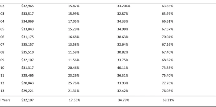
The median household income for the study area was $32.107. 17.55 percent of households did have access to a vehicle and 34.79 percent of block group residents identify
with another race other than white. 69.21 percent of housing units in the study were renter occupied (See Table 4-6).
Table 4-6. Socio-Demographic/Neighborhood Descriptive Statistics
Year Median HH Income (Median) Percent No Vehicle HH (Mean) Percent Non-White (Mean ) Percent Renter Occupied (Mean)
2002 $32,965 15.87% 33.204% 63.83% 2003 $33,517 15.99% 32.87% 63.97% 2004 $34,069 17.05% 34.33% 66.61% 2005 $33,843 15.29% 34.98% 67.37% 2006 $31,175 16.68% 38.63% 70.04% 2007 $35,157 13.58% 32.64% 67.16% 2008 $35,510 11.58% 30.82% 67.40% 2009 $32,107 11.56% 33.75% 68.62% 2010 $31,317 20.46% 40.11% 73.55% 2011 $28,465 23.26% 36.31% 75.40% 2012 $28,843 25.76% 33.93% 77.76% 2013 $29,221 21.31% 32.42% 76.03% All Years $32,107 17.55% 34.79% 69.21% Time Periods
An independent variable was created that represented time periods of important events in the implementation of the BRT and the real estate market fluctuations during the time span of this analysis (See Figure 4.4). This variable was used to evaluate the relationship between specific time periods and their effect on property values of residential property values within the study area (See Table 4-7 and See Figure 4.5).
Table 4-7. Time Period of Important BRT/Real Estate Market Events
Period Date Range BRT Event Real Estate Market Event Count of Sales
1 April 1, 2002- October 29, 2004 Pre-announcement Market rise 1,362
2 October 30, 2004-December 31, 2006 Construction Market boom 854
3 January 1, 2007- October 4, 2009 Construction Market bust 633
4 October 5, 2009-December 11, 2011 Post-opening Market bust 797
5 December 12, 2011-February 22, 2013 Post-opening Market recovery 464
Total 4,112
Figure 4.4. Sales Price (Unadjusted) of Properties Sold in Study Area with Periods $0 $50,000 $100,000 $150,000 $200,000 $250,000 $300,000 2002 2003 2004 2005 2006 2007 2008 2009 2010 2011 2012 2013 Sal es P ri ce Sales Year
Figure 4.5. Period Histogram
Distance Data
An independent variable that described distance from parcels to RTC stations was identified. Each parcel was spatially matched to the nearest RTC station using GIS software. The output returns network distance and the name of the closest RTC station for each parcel.
The shortest route from a residential property to the nearest station was 0.08 mile while the farthest route was 1 mile. The average distance from a property to the closest station was 0.70 mile (See Table 4-8).
Table 4-8. Distance Data Descriptive Statistics
Station Count of Properties Minimum (mi) Maximum (mi) Mean (mi)
Center/Burns 421 0.14 1 0.62 Center/Liberty 141 0.19 1 0.63 Meadowood Mall 350 0.39 0.99 0.73 Virginia/Best Buy 133 0.77 1 0.92 Virginia/Brinkby 251 0.43 1 0.78 Virginia/California 688 0.19 0.99 0.61 Virginia/Holcomb 374 0.19 1 0.62 Virginia/Mary 564 0.08 1 0.63 Virginia/Mt. Rose 396 0.35 1 0.72 Virginia/Orchard Plaza 173 0.32 1 0.55 Virginia/Parklane 70 0.42 0.58 0.49 Virginia/Peckham 9 0.92 0.99 0.95 Virginia/Peckham NS 172 0.42 1 0.87 Virginia/Peppermill 370 0.32 1 0.70 All Stations 4,112 0.10 1.0 0.7
Chapter Five: Methodology
Descriptive Data Analysis
Data exploration was performed to determine which variables required transformations before modelling. Through the use of scatterplots, histograms, and descriptive statistics,
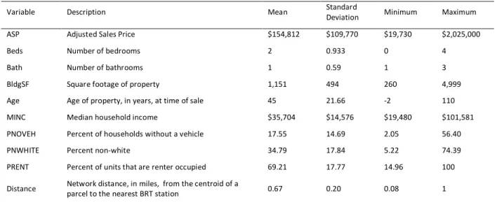
appropriate methods were used to normalize the data. Also scatterplots were used to display the bivariate relationship between the dependent and independent variables. Table 5-1 and Table 5-2 display the descriptive statistics of the variables before transformations.
Table 5-1. Variable Descriptive Statistics
Variable Description Mean Standard
Deviation Minimum Maximum ASP Adjusted Sales Price $154,812 $109,770 $19,730 $2,025,000
Beds Number of bedrooms 2 0.933 0 4
Bath Number of bathrooms 1 0.59 1 3
BldgSF Square footage of property 1,151 494 260 4,999 Age Age of property, in years, at time of sale 45 21.66 -2 110 MINC Median household income $35,704 $14,576 $19,480 $101,581 PNOVEH Percent of households without a vehicle 17.55 14.69 2.05 56.40 PNWHITE Percent non-white 34.79 17.84 5.22 74.39 PRENT Percent of units that are renter occupied 69.21 17.77 14.96 100 Distance Network distance, in miles, from the centroid of a
Table 5-2. Variable Descriptive Statistics, Continued Garage
(Y/N)
Basement
(Y/N) Half Bath (Y/N) Property Type
1,422/2,680 1,121/2,991 605/3,507
Condo 291
Duplex 210
Single Family 2,134
Townhouse 1,477
Hedonic Price Method
The real estate market is inherently a very complex, heterogeneous, system. A property represents many different factors that give it its value. These include: location, demand,
financing, property characteristics, and neighborhood characteristics. Because of this
complexity, it is often difficult to determine which characteristics affect value more than others without the use of statistical methods such as the hedonic price method. This technique is now the foundation for most research that analyzes the markets of heterogeneous goods. Rosen (1974) determined that the hedonic price method can be used to relate the price or value of a property (dependent variable) to homogeneous characteristics (independent variables) that are believed to impact its value. When all other independent variables are held constant, the change in the dependent variable, influenced by a single independent variable, can be
interpreted as the discount or premium that someone is willing to pay for a property given that that single independent variable changes.
When using hedonic price methods it is also necessary to be cognizant of its disadvantages. As previously mentioned, independent variables are used in modeling to
determine their influence on the dependent variable. However, hedonic price method does not account for omitted variables (Barreto & Howland, 2005). Therefore, when relevant variables
are omitted, the model may over or underestimate the influence of the other variables thus creating a bias. It is nearly impossible to account for every possible independent variable, therefore this research exercised best judgment and reviewed previous literature to ensure that appropriate explanatory variables that are crucial to the primary objective of this study, were included in modeling.
Modeling
Descriptive diagnostics were used to determine appropriate transformations for the variables before modeling was done. The variables “age”, “MINC”, and “PRENT” were
transformed to polynomials since the relationship between these variables and the dependent variable curvilinear. The variable “BldgSF” was also transformed using a log transformation since the data was not normally distributed. The dependent variable, “ASP” was also not normally distributed therefore it was transformed using a natural log.
Four hedonic price models were constructed to evaluate the influence that independent variables have on the dependent variable, adjusted sales price. The first model was constructed without the “period” variable. This was done to test the hypothesis that properties that are closer to the BRT stations, possessed higher sale prices without taking into account the time periods of BRT announcement, construction, and operations and the fluctuations of the real estate market. Using the same terms as the first model, the second model added the period
against period 1. This model allows the hypothesis to be tested taking into account the different periods of BRT implementation and the fluctuations of real estate market. The third model interacted the terms “distance” and “period”, for periods 2-5. This was done to determine if a property’s price may have been influenced by both distance to a BRT station and a certain time period. Finally, a fourth model was constructed with the same terms as the third model with the addition of a polynomial term for the interaction between the variables “distance” and “period”. This was done since it was predicted that the relationship between the interacted terms of “distance” and “period” was curvilinear (See Table 5-3)
Table 5-3: Hedonic Price Models Model
Number Model
1
ln(𝐴𝑆𝑃) = 𝑥 + 𝛽log (BldgSF) + 𝛽Beds + 𝛽Bath + 𝛽HBath + 𝛽Duplex + 𝛽SingleFH + 𝛽TownH + 𝛽Garage + 𝛽Basement + 𝛽Age + 𝛽Age2+ 𝛽MInc + 𝛽MInc2+ 𝛽PNoVeh + 𝛽𝑃NWhite + 𝛽PRrent + 𝛽PRent2+ 𝛽Distance
2
ln(𝐴𝑆𝑃) = 𝑥 + 𝛽log (BldgSF) + 𝛽Beds + 𝛽Bath + 𝛽HBath + 𝛽Duplex + 𝛽SingleFH + 𝛽TownH + 𝛽Garage + 𝛽Basement + 𝛽Age + 𝛽Age2+ 𝛽MInc + 𝛽MInc2+ 𝛽PNoVeh + 𝛽𝑃NWhite + 𝛽PRrent + 𝛽PRent2+ 𝛽Distance
+ 𝛽Period 2 + 𝛽Period 3 + 𝛽Period 4 + 𝛽Period 5
3
ln(𝐴𝑆𝑃) = 𝑥 + 𝛽log (BldgSF) + 𝛽Beds + 𝛽Bath + 𝛽HBath + 𝛽Duplex + 𝛽SingleFH + 𝛽TownH + 𝛽Garage + 𝛽Basement + 𝛽Age + 𝛽Age2+ 𝛽MInc + 𝛽MInc2+ 𝛽PNoVeh + 𝛽𝑃NWhite + 𝛽PRent + 𝛽PRent2+ 𝛽Distance
+ 𝛽Period 2 + 𝛽Period 3 + 𝛽Period 4 + 𝛽Period 5 + 𝛽(Distance ∗ Period 2) + 𝛽(Distance ∗ Period 3) + 𝛽(Distance ∗ Period 4) + 𝛽(Distance ∗ Period 5)
4
ln(𝐴𝑆𝑃) = 𝑥 + 𝛽 log(BldgSF) + 𝛽Beds + 𝛽Bath + 𝛽HBath + 𝛽Duplex + 𝛽SingleFH + 𝛽TownH + 𝛽Garage + 𝛽Basement + 𝛽Age + 𝛽Age2+ 𝛽MInc + 𝛽MInc2+ 𝛽PNoVeh + 𝛽𝑃NWhite + 𝛽PRent + 𝛽PRent2+ 𝛽Distance
+ 𝛽Period 2 + 𝛽Period 3 + 𝛽Period 4 + 𝛽Period 5 + 𝛽(Distance ∗ Period 2) + 𝛽(Distance ∗ Period 3) + 𝛽(Distance ∗ Period 4) + 𝛽(Distance ∗ Period 5) + 𝛽(Distance ∗ Period 2)2+ 𝛽(Distance ∗ Period 3)2+ 𝛽(Distance ∗ Period 4)2
+ 𝛽(Distance ∗ Period 5)2
After the initial construction of the models, regression diagnostics were used to detect outliers. Through the use of online software such as Google Earth street view, firsthand knowledge of the area, and the Washoe Property Appraiser’s office website, several records
were removed after it was determined that they contained erroneous or unverifiable data. For example, nine records were removed from the dataset because the sales transactions were representative of title transfers or deed modifications and not of a conventional sale. A record was also removed because the sale transaction was for an entire building and not a single residential property. There were a total of 4,102 records with the omission of these outliers.
Chapter Six:Results & Discussion
Descriptive Data Analysis
As mentioned in the methodology, transformations were performed for variables that were not normally distributed. This included the dependent variable, adjusted sales price. Figure 6.1 and Figure 6.2 display the distribution before and after the natural log of adjusted sales price was used to normalize data. Before the transformation was made, most properties in the study possessed an adjusted sales price between $0 and $35,000.
Figure 6.2. Adjusted Sales Price Transformed Histogram
Figure 6.3 and Figure 6.4 display the distribution of “log(BldgSF)” before and after transformation. As can be seen, there was about 900 properties that had a size of about 750-800 square feet. There was also about 500 properties with a size of about 1,200 square feet. Figure 6.5 is a scatterplot of the bivariate relationship between “log(BldgSF)” and adjusted sales price and it displays a positive linear association between the variables.
Figure 6.3. BldgSF Non-Transformed Histogram
Figure 6.5. Log(BldgSF) Scatterplot
Figure 6.6 displays a histogram of the distribution of the “beds” variable. As can be seen, most properties had 2 bedrooms. Figure 6.7 is a scatterplot of the bivariate relationship
between the dependent variable and “beds.” There was a positive association indicating that the more bedrooms a property had, the higher the adjusted sales price.
Figure 6.7. Beds Scatterplot
Figure 6.8 displays a histogram of the distribution of the “baths” variable. As can be seen, most properties had 1 bathroom. Figure 6.9 is a scatterplot of the bivariate relationship between the dependent variable and “baths.” There was a positive association indicating that the more bathrooms a property had, the higher the adjusted sales price.
Figure 6.10 displays a histogram of the distribution of the “baths” variable. As can be seen, most properties did not have a half bathroom. Figure 6.11 is a scatterplot of the bivariate relationship between the dependent variable and “baths.” There was a minimal positive
association indicating that if a property had a half bathroom, it sold for slightly more than a property without a half bathroom.
Figure 6.10. Half Baths Histogram
Figure 6.12 is a histogram that displays the distribution of the variable “BldgType.” As can be seen, most properties sold in the study area were single family homes. Figure 6.13 is a scatterplot that displays the bivariate relationship between the dependent variable and the “BldgType.” Properties that were condos, duplexes , or single family homes had similar adjusted sales prices, while townhomes possessed lower adjusted sales prices.
Figure 6.14 displays a histogram of the distribution of the “garage” variable. As can be seen, most properties did not have a garage. Figure 6.15 is a scatterplot of the bivariate relationship between the dependent variable and “garage.” There was a minimal positive association indicating that if a property had a garage, it sold for slightly more than a property without a garage.
Figure 6.13. Building Type Boxplot
Figure 6.15. Garage Scatterplot
Figure 6.16 displays a histogram of the distribution of the “basement” variable. As can be seen, most properties did not have a basement. Figure 6.17 is a scatterplot of the bivariate relationship between the dependent variable and “basement.” There was a minimal positive association indicating that if a property had a basement, it sold for slightly more than a property without a basement.
Figure 6.18 and Figure 6.19 display the distribution of “age” before and after
transformation. Figure 6.20 is a scatterplot of the bivariate relationship between “age2” and the dependent variable. As can be seen, there was a fluctuating association between the variables. Newer properties had higher adjusted sales prices, but depreciated in value as they aged.
Figure 6.16. Basement Histogram
Figure 6.20. Age2 Scatterplot
Figure 6.21 and Figure 6.22 display the distribution of “MINC” before and after
transformation. When the “MINC” variable was mapped, an interesting pattern was observed (See Figure 6.23). Lower income households, with incomes ranging between $25,001 and $50,000, were located closer to the BRT while higher income groups were located farther away. Figure 6.24 is a scatterplot of the bivariate relationship between “MINC2” and the dependent variable. As can be seen, there was a fluctuating association between the variables. In general, census tracts that had households with lower median incomes, also had lower adjusted sales price. As median household income increased, adjusted sales price also increased although, this increase was not significant.
Figure 6.24. MINC2 Scatterplot
Figure 6.25 displays the distribution of the variable “PNOVEH.” As can be seen, the frequency of census tracts with less than 25 percent no-vehicle households made up the majority of the distribution. However, there was a high frequency of census tracts with 28-30 percent no-vehicles households and about 55 percent no-vehicle households. Figure 6.26 is a scatterplot that displays the bivariate relationship between the dependent variable and the variable “PNOVEH.” As can be seen, there was fluctuating association between the variables indicating that census tracts that had fewer households with no-vehicles, possessed higher adjusted sales prices. Interestingly however, while there was a slight decline in adjusted sales
the “PNOVEH” variable displayed that census tracts with 0-10 percent households without access to a vehicle, were mostly clustered on the northwestern part of the BRT route. Census tracts with 20-30 percent households without access to a vehicle, were clustered together in the northeastern part of the BRT route (See Figure 6.27).
Figure 6.25. PNOVEH Histogram
Figure 6.28 displays the distribution of the variable “PNWHITE.” As can be seen, most census tracts had about 15-25 percent of the population that was not white. However, there was a significant amount of census tracts with a non-white population of 35-60 percent.
Figure 6.28. PNWHITE Histogram
Figure 6.29 is a scatterplot of the bivariate relationship between the dependent variable and the variable, “PNWHITE.”As can be seen, as the percentage of the non-white population in the census tracts increased, adjusted sales price decreased. There was a slight positive
association between the variables when the percentage of the non-white population reached 40 percent however, this association turned negative after about 50 percent.
Figure 6.29. PNWHITE Scatterplot
A map for the variable “PNOVEH” displays that census tracts that had a non-white population of 40 percent or greater, were located in the northeastern part of the BRT route. Census tracts that had non-white population of less than 40 percent, were clustered on the northwestern side of the part of the BRT route (See Figure 6.30).
Figure 6.31 and Figure 6.32 displays the distribution of the variable “PRENT2” before and after transformation. Before the transformation was made, there was high frequency of census tracts with more than 60 percent renter occupied housing units. Figure 6.33 is a scatterplot for the relationship between the variable, “PRENT2” and the dependent variable. As can be seen, a fluctuating association exists between the variables. The association remained stable through about 40 percent renter occupied housing units. However, this association sharply declined toward 60 percent renter occupied housing units. There was a slight increase in adjusted sales price as the percentage of renter occupied units reached 70 percent. However, price decreased as the percentage of renter occupied units increased. A map for “PRENT,” displays that census tracts that contained more than 50 percent renter occupied housing units, were clustered closest to the BRT route (See Figure 6.34). This may suggest that renters may more inclined to rent units that near BRT.
Figure 6.32. PRENT2 Histogram
Figure 6.35 displays the distribution of the variable “distance.” As can be seen, the frequency of properties increased as distance from the nearest BRT station also increased. Most properties were located 0.85 mile away from the nearest BRT station. Figure 6.36 is a scatterplot that displays the bivariate relationship between the dependent variable and the variable “distance.” The scatterplot indicates a fluctuating association between the variables with adjusted sales price decreasing, as distance increases. At about 0.6 mile, there was a slight increase in adjusted sales price. However after this point, adjusted sales price decreased and slightly increased as distance from the nearest BRT station reached 1 mile.
Figure 6.36. Distance Scatterplot
Hedonic Price Regressions
Table 6.1 displays results from the four hedonic regression models. The adjusted R2 remained generally consistent between models. The fourth model had the highest adjusted R2 value of 0.7673 while models 1 and 2 both had the lowest adjusted R2 value of 0.7634.
For the variables that describe property characteristics, the variable, log(BldgSF) was most influential in predicting adjusted sales price with a t-value of 25.60 in the fourth model. The influence of the variables, “beds” and “hbaths,” was consistent between models and had moderate significance in predicating adjusted sales price. The variable, “baths,” had a moderate significance in predicting adjusted sales price. For the variables that describe building type, “SingleFH” was the most influential and significant in predicting adjusted sales price with the