Inventories and optimal monetary policy

Inventories and Optimal

Monetary Policy

Thomas A. Lubik and Wing Leong Teo

I

explaining fluctuations in real gross domestic product (GDP), although it makes up only a small fraction of it. Blinder and Maccini (1991) document that in a typical recession in the United States, the fall in inventory investment accounts for 87 percent of the decline in output despite being only one half of 1 percent of real GDP. A lot of research has been trying to explain how this seemingly insignificant component of GDP has such a disproportionate role in

business cycle fluctuations.1 However, surprisingly few studies have focused

on the conduct of monetary policy when firms can invest in inventories. In this article we attempt to fill this gap by investigating how inventory investment affects the design of optimal monetary policy.

We employ the simple New Keynesian model that has become the bench-mark for analyzing monetary policy from both a normative and a positive perspective. We introduce inventories into the model by assuming that the in-ventory stock facilitates sales, as suggested in Bils and Kahn (2000). We first establish that the dynamics, and therefore the monetary transmission mech-anism, differ between the models with and without inventories for a given behavior of the monetary authority. Monetary policy is then endogenized by assuming that policymakers solve an optimal monetary policy problem.

First, we compute the optimal Ramsey policy. A Ramsey planner max-imizes the welfare of the agents in the economy by taking into account the

We are grateful to Andreas Hornstein, Pierre Sarte, Alex Wolman, and Nadezhda Malysheva, whose comments greatly improved the paper. Lubik is a senior economist at the Federal Reserve Bank of Richmond. Teo is an assistant professor at National Taiwan University. Lubik wishes to thank the Department of Economics at the University of Adelaide, where parts of this research were conducted, for their hospitality. The views expressed in this paper are those of the authors and should not necessarily be interpreted as those of the Federal Re-serve Bank of Richmond or the Federal ReRe-serve System. E-mails: thomas.lubik@rich.frb.org; wlteo@ntu.edu.tw.

private sector’s optimality conditions. In doing so, the planner chooses a so-cially optimal allocation. While this does not necessarily bear any relationship to the typical conduct of monetary policymakers, it provides a useful bench-mark. Subsequently, we study optimal policy when the planner is constrained to implement simple rules. That is, we specify a set of rules that lets the policy instrument (the nominal interest rate) respond to target variables such as the inflation rate and output. The policymaker chooses the respective response coefficients that maximize welfare. Optimal rules of this kind may be prefer-able to Ramsey plans from an actual policymaker’s perspective since they can be operationalized and are easier to communicate to the public.

Our most interesting but surprising finding is that Ramsey-optimal mon-etary policy deviates from full inflation stabilization in our model with inven-tories. This stands in contrast to the standard New Keynesian model. In the New Keynesian model, perfectly stable inflation is optimal since movements in prices represent deadweight costs to the economy. Introducing inventories potentially modifies that basic calculus for the following reasons. First, we assume that a firm’s inventory holdings are relevant for its sales only in rela-tive terms, that is, when they deviate from the aggregate inventory stock. This presents an externality, which a Ramsey planner may want to address. Second, inventories change the economy’s propagation mechanism as they allow firms to smooth sales over time with concomitant effects on consumption; that is, output and consumption need no longer coincide, which has a similar effect as capital in that it provides future consumption opportunities. Changes in prices serve as the equilibrating mechanism for the competing goals of reduc-ing consumption volatility and avoidreduc-ing price adjustment costs. The inventory specification therefore contains something akin to an inflation-output trade-off. Consequently, the optimal policy no longer fully stabilizes inflation. The second important finding concerns the efficacy of implementing simple rules. Similar to most of the optimal policy literature, we show that simple rules can come exceedingly close to the socially optimal Ramsey policy in welfare terms.

Our article relates to two literatures. First, the amount of research on op-timal monetary policy in the New Keynesian framework is very large already, and we do not have much to contribute conceptually to the modeling of optimal policy. Schmitt-Groh´e and Uribe (2007) is a recent important and compre-hensive contribution. A main conclusion from this literature is that optimal monetary policy will choose to almost perfectly stabilize inflation. In envi-ronments with various nominal and real distortions, this policy prescription becomes slightly modified, but nevertheless perseveres. We thus contribute to the optimal policy literature by demonstrating that the results carry over to a framework with another, previously unconsidered modification to the basic framework in the form of inventories.

The study of inventory investment has a long pedigree, to which we cannot do full justice here. Much of the earlier literature, as surveyed in Blinder and Maccini (1991), was concerned with identifying the determinants of inven-tory investment, such as aggregate demand and expectations thereof, or the opportunity costs of holding inventories. Most work in this area was largely empirical using semi-structural economic models, with West (1986) being a

prime example.2Almost in parallel to this more explicitly empirical literature,

inventories were introduced into real business cycle models. The seminal ar-ticle by Kydland and Prescott (1982) introduces inventories directly into the production function. More recent contributions include Christiano (1988), Fisher and Hornstein (2000), and Khan and Thomas (2007). The latter two articles especially build a theory of a firm’s inventory behavior on the micro-foundation of an S-s environment. The focus of these articles is on the business cycle properties of inventories, in particular the high volatility of inventory investment relative to GDP and the countercylicality of the inventory-sales ratio, both of which are difficult to match in typical inventory models. In an important article, Bils and Kahn (2000) demonstrate that time-varying and countercyclical markups are crucial for capturing this co-movement pattern.

This insight lends itself to considering inventory investment within a New Keynesian framework since it features interplay between marginal cost, in-flation, and monetary policy, which might therefore be a source of inventory

fluctuations.3 _{Recently, several articles have introduced inventories into New}

Keynesian models. Jung and Yun (2005) and Boileau and Letendre (2008) both study the effects of monetary policy from a positive perspective. The former combines Calvo-type price setting in a monopolistically competitive environment with the approach to inventories as introduced by Bils and Kahn (2000). The use of the Calvo approach to modeling nominal rigidity allows these authors to discuss the importance of strategic complementarities in price setting. Boileau and Letendre (2008), on the other hand, compare various ap-proaches to introducing inventories in a sticky-price model. This article is differentiated from those contributions by its focus on the implications of inventories as a transmission mechanism for optimal monetary policy.

The rest of the article is organized as follows. In the next section we develop our New Keynesian model with inventories. Section 2 analyzes the differences between the standard New Keynesian model and our specification with inventories. We calibrate both models and compare their implications for business cycle fluctuations. We present the results of our policy exercises in

2 A more recent example of applying structural econometric techniques to partial equilibrium inventory models is Maccini and Pagan (2008).

3 Incidentally, Maccini, Moore, and Schaller (2004) find that an inventory model with regime switches in interest rates is quite successful in explaining inventory behavior despite much previous empirical evidence to the contrary. The key to this result is the exogenous shift in interest rate regimes, which lines up with breaks in U.S. monetary policy.

Section 3, which also includes a robustness analysis with respect to changes in the parameterization. Section 4 concludes with a brief discussion of the main results and suggestions for future research.

1. THE MODEL

We model inventories in the manner of Bils and Kahn (2000) as a mechanism for facilitating sales. When firms face unexpected demand, they can simply draw down their stock of previously produced goods and do not have to en-gage in potentially more costly production. This inventory specification is embedded in an otherwise standard New Keynesian environment. There are three types of agents: monopolistically competitive firms, a representative household, and the government. Firms face price adjustment costs and use labor for the production of finished goods, which can be sold to households or added to the inventory. Households provide labor services to the firms and en-gage in intertemporal consumption smoothing. The government implements monetary policy.

Firms

The production side of the model consists of a continuum of monopolistically

competitive firms, indexed byi ∈[0,1]. The production function of a firmi

is given by

yt(i)=ztht(i) , (1)

whereyt(i)is output of firmi,ht(i)is labor hours used by firmi, andzt is

aggregate productivity. We assume that it evolves according to the exogenous stochastic process

lnzt =ρzlnzt−1+εzt, (2)

whereεzt is an i.i.d. innovation.

We introduce inventories into the model by assuming that they

facili-tate sales as suggested by Bils and Kahn (2000).4 In their partial equilibrium

framework, they posit a downward-sloping demand function for a firm’s prod-uct that shifts with the level of inventory available. As shown by Jung and Yun (2005), this idea can be captured in a New Keynesian setting with mo-nopolistically competitive firms by introducing inventories directly into the

4 This approach is consistent with a stockout avoidance motive. Wen (2005) shows that it explains the fluctuations of inventories at different cyclical frequencies better than alternative theories.

Dixit-Stiglitz aggregator of differentiated products: st = 1 0 at(i) at μ θ st(i)(θ−1)/θdi θ /(θ−1) , (3)

wherest are aggregate sales; st(i) are firm-specific sales; at andat(i) are,

respectively, the aggregate and firm-specific stocks of goods available for

sales;θ >1 is the elasticity of substitution between differentiated goods; and

μ >0 is the elasticity of demand with respect to the relative stock of goods.

Holding inventories helps firms to generate greater sales at a given price since they can rely on the stock of previously produced goods when, say, demand increases. Note, however, that a firm’s inventory matters only to the extent that it exceeds the aggregate level. In a symmetric equilibrium, having inventories does not help a firm to make more sales, but it affects the firm’s optimality condition for inventory smoothing.

Cost minimization implies the following demand function for sales of

goodi: st(i)= at(i) at μ Pt(i) Pt −θ st, (4)

wherePt(i)is the price of goodi, andPtis the price index for aggregate sales

st: Pt = 1 0 at(i) at μ Pt(i)1−θdi 1/(1₋θ ) . (5)

A firm’s sales are thus increasing in its relative inventory holdings and decreas-ing in its relative price. The inventory term can alternatively be interpreted as a taste shifter, which firms invest in to capture additional demand (see Kryvtsov and Midrigan 2009). Finally, the stock of goods available for sales

at(i)evolves according to

at(i)=yt(i)+(1−δ) (at−1(i)−st−1(i)) , (6)

whereδ∈(0,1)is the rate of depreciation of the inventory stock. It can also

be interpreted as the cost of carrying the inventory over the period.

Each firm faces quadratic costs for adjusting its price relative to the steady

state gross inflation rateπ: φ₂

Pt(i)

π Pt−1(i)−1

2

st, withφ >0, andπ ≥ 1, the

steady state gross inflation rate. Note that the costs are measured in units of

aggregate sales instead of output sincestis the relevant demand variable in the

model with inventories. Firmi’s intertemporal profit function is then given

by Et ∞ τ=0 ρt,t+τ Pt+τ(i) st+τ(i) Pt+τ − Wt+τht+τ(i) Pt+τ − φ 2 Pt+τ(i) π Pt+τ−1(i) −1 2 st+τ , (7)

whereWtis the nominal wage andρt,t+τ is the aggregate discount factor that

a firm uses to evaluate profit streams.

Firm i chooses its price, Pt(i), labor input, ht(i), and stock of goods

available for sales, at(i), to maximize its expected intertemporal profit (7),

subject to the production function (1), the demand function (4), and the law

of motion forat(i)(6). The first order conditions are

φ Pt(i) π Pt−1(i) −1 st π Pt−1(i) =(1−θ )st(i) Pt +Etρt,t+1 φ Pt+1(i) π Pt(i) −1 st+1Pt+1(i) π Pt2(i) +(1−δ) θst(i) Pt(i) mct+1(i) (8) Wt Pt =ztmct(i), (9) and mct(i)=μ Pt(i) Pt st(i) at(i) +(1−δ) 1−μst(i) at(i) Etρt,t+1mct+1(i), (10)

wheremct(i)is the Lagrange multiplier associated with the demand constraint

(4). It can also be interpreted as real marginal cost.

Equation (8) is the optimal price-setting condition in our model with in-ventories. It resembles the typical optimal price-setting condition in a New Keynesian model with convex costs for price adjustment (e.g., Krause and Lubik 2007), except that marginal cost now enters the optimal pricing con-dition in expectations because of the presence of inventories. In this model,

the behavior of marginal cost,mc, can be interpreted from two different

di-rections. As captured by Equation (9), it is the ratio of the real wage to the marginal product of labor, which in the standard model is equal to the cost of producing an additional unit of output. Alternatively, it is the cost of generat-ing an additional unit of goods available for sale, which can either come out of current production or out of (previously) foregone sales. This in turn reduces the stock of goods available for sales in future periods, which would eventually have to be replenished through future production. This intertemporal tradeoff between current and future marginal cost is captured by Equation (10).

Household

We assume that there is a representative household in the economy. It

consumption,5_c

t, and labor hours,ht:

E0 ∞ t=0 βt ζtlnct − h1t+η 1+η , (11)

whereη≥0 is the inverse of the Frisch labor supply elasticity.

ζt is a preference shock and is assumed to follow the exogenous AR(1)

process

lnζt =ρζlnζt−1+εζ ,t, (12)

where 0< ρζ <1 andεζ ,t is an i.i.d. innovation.

The household supplies labor hours to firms at the nominal wage rate,

Wt, and earns dividend income,Dt, (which is paid out of firms’ profits) from

owning the firms. It can purchase one-period discount bonds,Bt, at a price of

1/Rt, whereRt is the gross nominal interest rate. Its budget constraint is

Ptct+Bt/Rt ≤Bt−1+Wtht+Dt. (13)

The first-order conditions for the representative household’s utility maximiza-tion problem are

hηt = ζt ct Wt Pt , and (14) ζ_t ct = βRtEt ζ_t+1 ct+1 Pt Pt+1 . (15)

Equation (14) equates the real wage, valued in terms of the marginal util-ity of consumption, to the disutilutil-ity of labor hours. Equation (15) is the consumption-based Euler equation for bond holdings.

Government and Market Clearing

In order to close the model, we also need to specify the behavior of the mone-tary authority. The main focus of the paper is the optimal monemone-tary policy in the New Keynesian model with inventories. In the next section, however, we briefly compare our specification to the standard model without inventories in order to assess whether introducing inventories significantly changes the model dynamics. We do this conditional for a simple, exogenous interest rate feedback rule that has been used extensively in the literature:

Rt =ρRt−1+ψ1πt+ψ2yt +εR,t, (16)

5 Consumption can be thought of as a Dixit-Stiglitz aggregate, as is typical in New Keynesian models. We abstract from this here for ease of exposition.

where a tilde over a variable denotes its log deviation from its deterministic

steady state.ψ1andψ2are monetary policy coefficients and 0< ρ <1 is the

interest smoothing parameter. εR,t is a zero mean innovation with constant

variance; it is often interpreted as a monetary policy implementation error. Finally, we impose a symmetric equilibrium, so that the firm-specific indices,

i, can be dropped. In addition, we assume that bonds are in zero net supply,

Bt = 0. Market clearing in the goods market requires that consumption,

together with the cost for price adjustment, equals aggregate sales:

st =ct+ φ 2 _π t π −1 2 st. (17)

2. ANALYZING THE EFFECTS OF MONETARY POLICY

The main focus of this article is how the introduction of inventories into an otherwise standard New Keynesian framework changes the optimal design of monetary policy. However, we begin by briefly comparing the behavior of the model with and without inventories to assess the changes in the dynamic behavior of output and inflation, given the exogenous policy rule (16). The standard New Keynesian model differs from our model with inventories in the following respects. First, there is no explicit intertemporal tradeoff in terms of marginal cost as in equation (10). This implies, secondly, that the driving term in the Phillips curve (8) is current marginal cost, as defined by equation (9). Finally, in the standard model, consumption, output, sales, and goods available of sales are first-order equivalent. We note, however, that the standard specification is not nested in the model with inventories; that is, the equation system for the latter does not reduce to the former for a specific parameterization.

Calibration

The time period corresponds to a quarter. We set the discount factor, β,

to 0.99. Since price adjustment costs are incurred only for deviations from steady-state inflation, its value is irrelevant for first-order approximations of the model’s equation system but plays a role when we perform the optimal

policy analysis. We therefore setπ =1.0086 to be consistent with the average

post-war, quarter-over-quarter inflation rate. In the baseline calibration, we

choose a fairly elastic labor supply and setη=1, which is a common value

in the literature and corresponds to quadratic disutility of hours worked. We

impose a steady-state markup of 10 percent, which implies θ = 11. The

price adjustment cost parameter is then calibrated so thatη(θ−1)/φ =0.1,

cost in the standard New Keynesian Phillips curve.6 _{The parameters of the}

monetary policy rule are chosen to be broadly consistent with the empirical

Taylor rule literature for a unique equilibrium. That is,ψ1andψ2are set to

0.45 and 0, respectively, while the smoothing parameter is set toρ=0.7. This

choice corresponds to an inflation coefficient of 0.45/0.3=1.5 that obeys the

Taylor principle. We specify the policy rule in this manner since it allows us

to analyze later the effects of inertial and super-inertial rules withρ ≥1.

The persistence of the technology shock and the preference shock are

both set to ρz = ρζ = 0.95. The standard deviation of the productivity

innovation is then chosen so as to match the standard deviation of HP-filtered

U.S. GDP of 1.61 percent. This yields a value ofσz = 0.005. We set the

standard deviation of the preference shocks at three times the value of the former, which is consistent with empirical estimates from a variety of studies (e.g., Ireland 2004). In the same manner, we choose a standard deviation of

the monetary policy shock of 0.003. The parameters related to inventories,μ

andδ, are calibrated following Jung and Yun (2005); specifically the elasticity

of demand with respect to the stock of goods available for sales isμ=0.37,

while the depreciation rate of the inventory stock isδ=0.01.

Do Inventories Make a Difference?

To get an idea how the introduction of inventories changes the model dynam-ics, we compare the responses of some key variables to technology, preference, and monetary policy shocks for the specification with and without inventories. The impulse responses are found in Figures 1–3, respectively. In the figures, the label “Base” refers to the responses under the specification without inven-tories, while “Inv” indicates the inventory specification. The key qualitative difference between the two models is the behavior of labor hours. In response to a persistent technology shock, labor increases in the model with inventories, while it falls in the standard New Keynesian model before quickly returning

to the steady state.7 In the New Keynesian model, firms can increase

pro-duction even when economizing on labor because of the higher productivity level. There is further downward pressure on labor since the productivity shock raises the real wage. Higher output is reflected in a drop in prices, which are drawn out over time due to the adjustment costs, and marginal cost falls strongly.

The presence of inventories, however, changes this basic calculus as firms can use inventories to take advantage of current low marginal cost. With

6 This value is also consistent with an average price duration of about four quarters in the Calvo model of staggered price adjustment.

7 Chang, Hornstein, and Sarte (2009) also emphasize that in the presence of nominal rigidities labor hours can increase in response to a persistent technology shock when firms hold inventories.

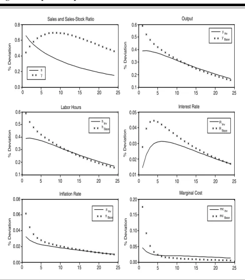
Figure 1 Impulse Response Functions to Productivity Shock s γ y_Inv y_Base h_Inv h_Base R_Inv R_Base πInv πBase mc_Inv mc_Base Sales and Sales-Stock Ratio Output

Interest Rate Labor Hours

Inflation Rate Marginal Cost

% De viation % De viation % De viation % De viation % De viation % De viation 0 5 10 15 20 25 0 5 10 15 20 25 0 5 10 15 20 25 0 5 10 15 20 25 0 5 10 15 20 25 0 5 10 15 20 25 1.0 0.5 0.0 -0.5 -1.0 -1.5 1.5 1.0 0.5 0.0 0.3 0.2 0.1 0.0 -0.1 -0.2 -0.02 -0.04 -0.06 -0.08 -0.10 0.00 -0.05 -0.10 -0.15 -0.20 0.0 -0.1 -0.2 -0.3 -0.4

inventory accumulation firms need not sell the additional output immediately, which prompts them to increase labor input. Consequently, output rises by more than in the standard model and the excess production is put in inventory. The stock of goods available for sales thus rises, whereas the sales-to-stock

ratio, γ_t ≡ st/at, falls. This is also reflected in the (albeit small) fall in

marginal cost, which is, however, persistent and drawn out. In other words, firms use inventories to take advantage of current and future low marginal cost. Inflation moves in the same direction as in the standard model, but is much smoother, as the increased output does not have to be priced immediately. This behavior is just the flip side of the smoothing of marginal cost.

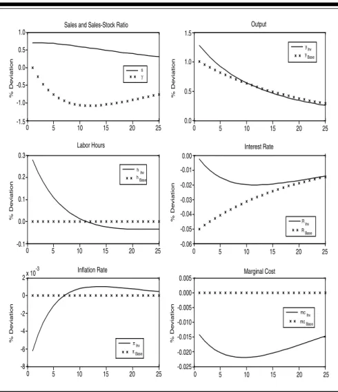
Figure 2 Impulse Response Functions to Preference Shock % De viation % De viation % De viation % De viation % De viation % De viation

Sales and Sales-Stock Ratio Output

Labor Hours Interest Rate

Inflation Rate Marginal Cost s γ yInv y_Base h_Inv h Base R_Inv R Base πInv πBase mc Inv mc_Base 0 5 10 15 20 25 0 5 10 15 20 25 0 5 10 15 20 25 0 5 10 15 20 25 0 5 10 15 20 25 0 5 10 15 20 25 0.8 0.6 0.4 0.2 0.0 0.6 0.5 0.4 0.3 0.2 0.1 0.6 0.5 0.4 0.3 0.2 0.1 0.05 0.04 0.03 0.02 0.01 0.08 0.06 0.04 0.02 0.00 0.20 0.15 0.10 0.05 0.00

In response to a preference shock, hours move in the same direction in both models. However, the response with inventories is smaller since firms can satisfy the additional demand out of their inventory holdings, which therefore does not drive up marginal cost as much. Compared to the standard model, firms do not have to resort to increases in price or labor input to satisfy the additional demand. Inventories are thus a way of smoothing revenue over time, which is also consistent with a smoother response of inflation. The dynamics following a contractionary policy shock are qualitatively similar to those of technology shocks in terms of co-movement. Sales in the inventory model fall, but output and hours increase to take advantage of the falling marginal

Figure 3 Impulse Response Functions to Monetary Policy Shock % De viation % De viation % De viation % De viation % De viation % De viation

Sales and Sales-Stock Ratio

Labor Hours Inflation Rate Output Interest Rate Marginal Cost s γ h Inv h Base Inv Base y Inv y Base R Inv R_Base mc_Inv mc Base 0 5 10 15 20 25 0 5 10 15 20 25 0 5 10 15 20 25 0 5 10 15 20 25 0 5 10 15 20 25 0 5 10 15 20 25 1 0 -1 -2 -3 1.0 0.5 0.0 -0.5 -1.0 -1.5 -2.0 1.0 0.5 0.0 -0.5 -1.0 -1.5 -2.0 0 -1 -2 -3 -4 0.8 0.6 0.4 0.2 0.0 -0.2 0.0 -0.2 -0.4 -0.6 -0.8 π π

cost. All series are again noticeably smoother when compared to the standard model.

We now briefly discuss some business cycle implications of the

inven-tory model.8 Table 1 shows selected statistics for key variables. A notable

stylized fact in U.S. data is that production is more volatile than sales. We find that our inventory model replicates this observation in the case of pro-ductivity shocks, that is, output is 30 percent more volatile. This implies that

8 This aspect is discussed more extensively in Boileau and Letendre (2008) and Lubik and Teo (2009).

Table 1 Business Cycle Statistics

Moments Technology Preference Policy All Shocks

Standard Deviation (%)

Output 1.61 1.93 0.23 2.52

Sales 1.18 2.37 0.74 2.80

Hours 0.25 1.93 0.23 2.02

Correlation

(Sales, _InventorySales ) −0.85 0.87 0.51 0.49

(_StockSales, Marginal Cost 0.95 0.90 0.72 0.49

consumption, which is equal to sales in our linearized setting, is also less volatile than GDP. The introduction of inventories is thus akin to the model-ing of capital and investment in breakmodel-ing the tight link between output and consumption embedded in the standard New Keynesian model. However, the model has counterfactual implications for the co-movement of inventory variables. Sales are highly negatively correlated with the sales-inventory ra-tio, whereas in the data the two series co-move slightly positively and are at best close to uncorrelated. This finding can be overturned when either preference or policy shocks are used, both of which imply a strong positive co-movement. However, in the case of policy shocks, sales are counterfactu-ally more volatile than output. When all shocks are considered together, we find that co-movement between the inventory variables are positive, but not unreasonably so, while sales are slightly more volatile than output.

The model also has implications for inflation dynamics. Most notably, inflation is less volatile in the inventory specification than in the standard model. In the New Keynesian model, inflation is driven by marginal cost; hence, the standard model predicts that the two variables are highly correlated. In the data, however, proxies for marginal cost, such as unit labor cost or the labor share, co-move only weakly with inflation. This has been a challenge for empirical studies of the New Keynesian Phillips curve. Our model with inventories may, however, improve the performance of the Phillips curve in two aspects. First, marginal cost smoothing translates into a smoother and thus more persistent inflation path; second, the form and the nature of the driving process in the Phillips curve equation changes, as is evident from equations (8) and (10). The latter equation predicts a relationship between marginal cost

and the sales-to-stock ratio,γ, which changes the channel by which marginal

cost affects inflation dynamics.9

9 This is further and more formally empirically investigated in Lubik and Teo (2009), who suggest that the inventory channel does not contribute much to explain observed inflation behavior.

We can tentatively conclude that a New Keynesian model with inventories presents a modified set of tradeoffs for an optimizing policymaker. In the standard model optimal policy is such that both consumption and the labor supply should be smoothed and price adjustment costs minimized. In the inventory model, these objectives are still relevant since they affect utility in the same manner, but the channel through which this can be achieved is different. Inventories allow for a smoother adjustment path of inflation, which should help contain the effects of price stickiness, while the consumption behavior depends on the nature of the shocks. We now turn to an analysis of optimal policy with inventories.

3. OPTIMAL MONETARY POLICY

The goal of an optimizing policymaker is to maximize a welfare function sub-ject to the constraints imposed by the economic environment and subsub-ject to assumptions about whether the policymaker can commit or not to the cho-sen action. In this article, we assume that the optimizing monetary authority maximizes the intertemporal utility function of the household subject to the optimal behavior chosen by the private sector and the economy’s feasibility constraints. Furthermore, we assume that the policymaker can credibly com-mit to the chosen path of action and does not re-optimize along the way. We consider two cases. For our benchmark, we assume that the monetary

author-ity implements the Ramsey-optimal policy.10 We then contrast the Ramsey

policy with an optimal policy that is chosen for a generic set of linear rules of the type used in the simulation analysis above.

We can alternatively interpret the policymaker’s actions as minimizing the distortions in the model economy. In a typical New Keynesian setup like ours, there are two distortions. The first is the suboptimal level of output generated by the presence of monopolistically competitive firms. The second distortion arises from the presence of nominal price stickiness, as captured by the quadratic price adjustment cost function, which is a deadweight loss to the economy. In the standard model, the optimal policy perfectly stabilizes in-flation at the steady-state level. Introducing inventories can change this basic calculus in our model, as the sales-relevant terms are relative inventory hold-ings that present an externality for a Ramsey planner. We will now investigate whether this additional wedge matters quantitatively for optimal policy.

Welfare Criterion

We use expected lifetime utility of the representative household at time

zero, V₀a, as the welfare measure to evaluate a particular monetary policy

10 See Khan, King, and Wolman (2003), Levin et al. (2006), and Schmitt-Groh´e and Uribe (2007) for wide-ranging and detailed discussions of this concept in New Keynesian models.

regime,a: V0a≡E0 ∞ t=0 βt ζtlnC a t − ha t 1+η 1+η . (18)

As in Schmitt-Groh´e and Uribe (2007), we compute the expected lifetime utility conditional on the initial state being the deterministic steady state for given sequences of optimal choices of the endogenous variables and exogenous shocks. Our welfare measure is in the spirit of Lucas (1987) and expresses

welfare as a percentage of steady-state consumption that the household

is willing to forgo to be as well off under the steady state as under a given

monetary policy regime,a. can then be computed implicitly from

∞ t=0 βt ζln 1− 100 c − h1+η 1+η =V₀a, (19)

where variables without time subscripts denote the steady state of the

cor-responding variables.11 Note that a higher value ofcorresponds to lower

welfare. That is, the household would be willing to give up percent of

steady-state consumption to implement a policy that delivers the same level of welfare as the economy in the absence of any shocks. This also captures the notion that business cycles are costly because they imply fluctuations that a consumption-smoothing and risk-averse agent would prefer not to have.

Optimal Policy

We compute the Ramsey policy by formulating a Lagrangian problem in which the government maximizes the welfare function (18) of the representative household subject to the private sector’s first-order conditions and the market-clearing conditions of the economy. The optimality conditions of this Ramsey policy problem can then be obtained by differentiating the Lagrangian problem with respect to each of the endogenous variables and setting the derivatives to zero. This is done numerically by using the Matlab procedures developed by Levin and Lopez-Salido (2004). The welfare function is then approxi-mated around the distorted, non-Pareto-optimal steady state. The source of steady-state distortion is the inefficient level of output due to the presence of monopolistically competitive firms.

In our second optimal policy case, we follow Schmitt-Groh´e and Uribe (2007) and consider optimal, simple, and implementable interest rate rules.

11 We assume that the policymaker chooses the same steady-state inflation rate for all mon-etary policies that we consider. The steady state of all variables will thus be the same for all policies.

Specifically, we consider rules of the following type:

Rt =ρRt−1+ψ1Etπt+i+ψ2Etyt+i, i = −1,0,1. (20)

The subscripti indicates that we consider forward-looking (i =1),

contem-poraneous (i = 0), and backward-looking rules (i = −1). Following the

suggestion in Schmitt-Groh´e and Uribe (2007), we focus on values of the

policy parametersρ,ψ1, andψ2that are in the interval [0,3]. Note that this

rule also allows for the possibility that the interest rate is super-inertial; that

is, we assumeρcan be larger than 1. In order to find the constrained-optimal

interest rate rule, we search for combinations of the policy coefficients that maximize the welfare criterion. As in Schmitt-Groh´e and Uribe (2007), we impose two additional restrictions on the interest rate rule: (i) the rule has to be consistent with a locally unique rational expectations equilibrium; (ii)

the interest rate rule cannot violate 2σR < R, whereσRis the unconditional

standard deviation of the gross interest rate whileRis its steady-state value.

The second restriction is meant to approximate the zero bound constraint on

the nominal interest rate.12

Ramsey-Optimal Policy

A key feature of the standard New Keynesian setup is that Ramsey-optimal policy completely stabilizes inflation. Price movements represent a

dead-weight loss to the economy because of the existence of adjustment costs.13

An optimizing planner would, therefore, attempt to remove this distortion. This insight is borne out by the impulse response functions for the standard model without inventories in Figure 4. Inflation does not respond to the tech-nology shock, nor do labor hours or marginal cost as per the New Keynesian Phillips curve. The path of output simply reflects the effect of increased and persistent productivity. The Ramsey planner takes advantage of the temporar-ily high productivity and allocates it straight to consumption without feedback to higher labor input or prices. The planner could have reduced labor supply to smooth the time path of consumption. However, this would have a level ef-fect on utility due to lower consumption, positive price adjustment cost via the feedback from lower wages to marginal cost, and increased volatility in hours. The solution to this tradeoff is thus to bear the brunt of higher consumption volatility.

The possibility of inventory investment, however, changes this rationale (see Figure 4). In response to a technology shock, output increases by more

12 If R is normally distributed, 2σR< R implies that there is a 95 percent chance that R will not hit the zero bound.

13 In a framework with Calvo price setting, the deadweight loss comes in the form of relative price distortions across firms, which lead to the misallocation of resources.

Figure 4 Impulse Response Functions to Productivity Shock: Ramsey Policy % De viation % De viation % De viation % De viation % De viation % De viation

Sales and Sales-Stock Ratio Output

Labor Hours Interest Rate

Inflation Rate Marginal Cost

s γ y Inv y_Base h_Inv h_Base R Inv R Base πInv πBase mc_Inv mc_Base 0 5 10 15 20 25 0 5 10 15 20 25 0 5 10 15 20 25 0 5 10 15 20 25 0 5 10 15 20 25 0 5 10 15 20 25 1.0 0.5 0.0 -0.5 -1.0 -1.5 1.5 1.0 0.5 0.0 0.3 0.2 0.1 0.0 -0.1 0.00 -0.01 -0.02 -0.03 -0.04 -0.05 -0.06 x 10-3 2 0 -2 -4 -6 -8 0.005 0.000 -0.005 -0.010 -0.015 -0.020 -0.025

compared to the model without inventories, while consumption, which is first-order equivalent to sales, rises less. Ramsey-optimal policy can induce a smoother consumption profile by allowing firms to accumulate inventories. Similarly, the planner takes advantage of higher productivity in that he in-duces the household to supply more labor hours. Inflation is now no longer completely stabilized as the lower increase in consumption leads to an initial decline in inflation. Inventories thus serve as a savings vehicle that allows the planner to smooth out the impact of shocks. The planner incurs price adjustment costs and disutility from initially high labor input. The benefit is a smoother and more prolonged consumption path than would be possible

Table 2 Welfare Costs and Standard Deviations under Ramsey-Optimal Policy

Technology Preference All Shocks

Panel A: Model without Inventories

Welfare Cost () 0.0000 −0.0521 −0.0521 Standard Deviation (%) Output 1.60 2.40 2.89 Inflation 0.00 0.00 0.00 Consumption 1.60 2.40 2.89 Labor 0.00 2.40 2.40

Panel B: Model with Inventories

Welfare Cost () 0.000 −0.0529 −0.0529 Standard Deviation (%) Output 1.73 2.28 2.86 Inflation 0.02 0.04 0.04 Consumption 1.45 2.60 2.97 Labor 0.24 2.28 2.29

Panel C: Full Inflation Stabilization

Welfare Cost () 0.000 −0.0528 −0.0528 Standard Deviation (%) Output 1.73 2.29 2.87 Inflation 0.00 0.00 0.00 Consumption 1.45 2.61 2.99 Labor 0.24 2.29 2.30

without inventories. The model with inventories therefore restores something akin to an output-inflation tradeoff in the New Keynesian framework.

The quantitative differences between the two specifications are small, however. Table 2 reports the welfare costs and standard deviations of selected variables for the two versions of the model under Ramsey-optimal policy. The welfare costs of business cycles in the standard model are vanishingly small when only technology shocks are considered and undistinguishable from the specification with inventories. The standard deviation of inflation is zero for the model without inventories while it is slightly higher for the model with inventories. This is consistent with the evidence from the impulse responses and highlights the differences between the two model specifications. Note also that consumption is less volatile in the model with inventories than in the standard model, which reflects the increased degree of consumption smoothing

in the former.14

14 This is consistent with the simulation results reported in Schmitt-Groh´e and Uribe (2007) in a model with capital. They also find that full inflation stabilization is no longer optimal since

Figure 5 Impulse Response Functions to Preference Shock: Ramsey Policy % De viation % De viation % De viation % De viation % De viation % De viation 0 5 10 15 20 25

Sales and Sales-Stock Ratio Output

Labor Hours Interest Rate

Inflation Rate Marginal Cost

s γ y Inv y Base h_Inv h_Base R_Inv R_Base πInv πBase mc_Inv mc_Base 0 5 10 15 20 25 0 5 10 15 20 25 0 5 10 15 20 25 0 5 10 15 20 25 0 5 10 15 20 25 0.8 0.6 0.4 0.2 0.0 0.5 0.4 0.3 0.2 0.1 0.5 0.4 0.3 0.2 0.1 0.05 0.04 0.03 0.02 0.01 0.00 x 10-3 2 0 -2 -4 -6 0.02 0.01 0.00 -0.01 -0.02 -0.03 -0.04

Figure 5 depicts the impulse responses to the preference shock under Ramsey-optimal policy. Inflation and marginal cost are fully stabilized in the standard model, which the planner achieves through a higher nominal interest rate that reduces consumption demand in the face of the preference shock. At the same time, the planner lets labor input go up to meet some of the additional demand. In contrast, Ramsey policy for the inventory model

investment in capital provides a mechanism for smoothing consumption, just as inventory holdings do in our model.

can allow consumption to increase by more since firms can draw on their stock of goods for sale. Consequently, output and labor increase by less for the inventory model. Similarly to the case of the technology shock, optimal policy does not induce complete inflation stabilization as it uses the inventory channel to smooth consumption. This is confirmed by the simulation results in Table 2, which show the Ramsey planner trading off volatility between inflation, consumption, and labor when compared to the standard model.

Interestingly, eliminating business cycles and imposing the steady-state allocation is costly for the planner in the presence of preference shocks that multiply consumption. This is evidenced by the negative entries for the welfare cost in both model specifications. In other words, agents would be willing to

pay the planner 0.05 percent of their steady-state consumptionnotto eliminate

preference-driven fluctuations. This stems from the fact that, although fluctu-ations per se are costly in welfare terms for risk-averse agents, they can also induce co-movement between the shocks and other variables that have a level effect on utility. Specifically, preference shocks co-move positively with con-sumption due to an increase in demand. This positive co-movement is reflected in a positive covariance between these two variables. In our second-order ap-proximation to the welfare functions, this overturns the negative contribution to welfare from consumption volatility.

When we consider both shocks together, the differences between the two specifications are not large in welfare terms and with respect to the implica-tions for second moments. Inflation and consumption are more volatile in the inventory version, while labor is less volatile compared to standard specifica-tion. We also compare Ramsey-optimal policy with inventories to a policy of fully stabilizing inflation only (as opposed to using the utility-based welfare criterion from above). Panel C of Table 2 shows that the latter is very close to the Ramsey policy. The welfare difference between the two policies is small— less than 0.001 percentage points of steady-state consumption. The effects of inventories can be seen in the slightly higher volatility of consumption and labor under the full inflation stabilization policy. Inventory investment allows the planner to smooth consumption more compared to the standard model, and the mechanism is a change in prices. Although price stability is feasible, the planner chooses to incur an adjustment cost to reduce the volatility of consumption and labor.

Optimal Policy with a Simple and Implementable Rule

Ramsey-optimal policy provides a convenient benchmark for welfare analysis in economic models. However, from the point of view of a policymaker, pur-suing a Ramsey policy may be difficult to communicate to the public. It may also not be operational in the sense that the instruments used to implement

the Ramsey policy may not be available to the policymaker. For instance, in a market economy the government cannot simply choose allocations as a Ram-sey plan might imply. The literature has therefore focused on finding simple and implementable rules that come close to the welfare outcomes implied by Ramsey policies (see Schmitt-Groh´e and Uribe 2007).

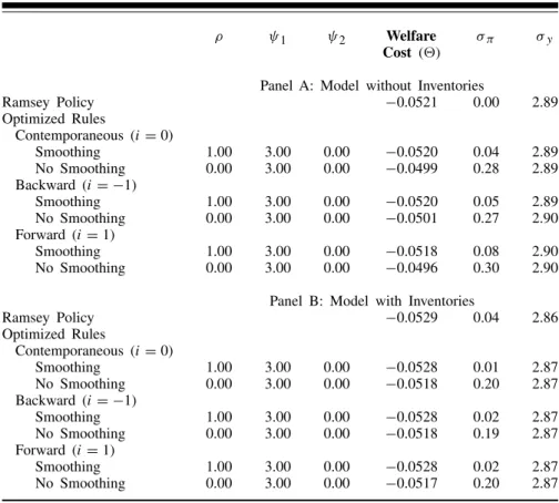
Therefore, we investigate the implications for optimal policy conditional on the simple rule (20). Panel A of Table 3 shows the constrained-optimal in-terest rate rules for the model without inventories with all shocks considered simultaneously. The rule that delivers the highest welfare is a

contempora-neous rule, with a smoothing parameterρ = 1 and reaction coefficients on

inflationψ1and outputψ2of 3 and 0, respectively.15 This is broadly consistent

with the results of Schmitt-Groh´e and Uribe (2007), where the constrained-optimal interest rate rule also features interest smoothing and a muted response to output. Without interest rate smoothing the welfare cost of implementing this policy increases, which is exclusively due to a higher volatility of inflation. On the other hand, the difference between the constrained-optimal con-temporaneous rule and the Ramsey policy is small—less than 0.001 percentage points. This confirms the general consensus in the literature that simple rules can come extremely close to Ramsey-optimal policies in welfare terms. The characteristics of constrained-optimal backward-looking and forward-looking rules are similar to the contemporaneous rule, i.e., they also feature full in-terest smoothing and no output response. The welfare difference between the constrained-optimal contemporaneous rule and the other two rules are also small.

Turning to the model with inventories, we report the results for the con-strained-optimal rules in Panel B of Table 3. All rules with interest smooth-ing deliver virtually identical results but strictly dominate any rule without smoothing. As before, the coefficient on output is zero, while the policymak-ers implement a strong inflation response. The main difference to the Ramsey outcome is that inflation is slightly less volatile, while output is more volatile. This again confirms the findings in other articles that a policy rule with a fully inertial interest rate and a hawkish inflation response delivers almost Ramsey-optimal outcomes.

Sensitivity Analysis

We now investigate the robustness of our optimal monetary policy results to alternative parameter values. The results of alternative calibrations are reported in Table 4, where we only document results for the rule that comes closest to the Ramsey benchmark. In the robustness analysis, we change

15 The reader may recall that we restricted the policy coefficients to lie within the interval [0,3].

Table 3 Optimal Policy with a Simple Rule

ρ ψ₁ ψ₂ Welfare σπ σy

Cost ()

Panel A: Model without Inventories

Ramsey Policy −0.0521 0.00 2.89 Optimized Rules Contemporaneous (i=0) Smoothing 1.00 3.00 0.00 −0.0520 0.04 2.89 No Smoothing 0.00 3.00 0.00 −0.0499 0.28 2.89 Backward (i= −1) Smoothing 1.00 3.00 0.00 −0.0520 0.05 2.89 No Smoothing 0.00 3.00 0.00 −0.0501 0.27 2.90 Forward (i=1) Smoothing 1.00 3.00 0.00 −0.0518 0.08 2.90 No Smoothing 0.00 3.00 0.00 −0.0496 0.30 2.90

Panel B: Model with Inventories

Ramsey Policy −0.0529 0.04 2.86 Optimized Rules Contemporaneous (i=0) Smoothing 1.00 3.00 0.00 −0.0528 0.01 2.87 No Smoothing 0.00 3.00 0.00 −0.0518 0.20 2.87 Backward (i= −1) Smoothing 1.00 3.00 0.00 −0.0528 0.02 2.87 No Smoothing 0.00 3.00 0.00 −0.0518 0.19 2.87 Forward (i=1) Smoothing 1.00 3.00 0.00 −0.0528 0.02 2.87 No Smoothing 0.00 3.00 0.00 −0.0517 0.20 2.87

one parameter at a time while holding all other parameters at their benchmark values. The overall impression is that in all alternative calibrations the optimal simple rule comes close to the Ramsey policy, and that the relative welfare rankings for the individual rules established in the benchmark calibration are unaffected. Specifically, inertial rules tend to dominate rules with a lower degree of smoothing.

We first look at the implications of alternative values for the two parameters related to inventories: the elasticity of demand with respect to the stock of

goods available for sale,μ, and the depreciation rate of the inventory stock,δ.

As in Jung and Yun (2005), we consider the alternative valueμ=0.8. Since

sales now respond more elastically to the stock of goods available for sale, the inventory channel becomes more valuable as a consumption-smoothing device and inflation becomes more volatile under a Ramsey policy. The best simple rule has contemporaneous timing and comes very close to the Ramsey policy in terms of welfare. The optimal rule is inertial and strongly reacts to inflation only. The volatility of inflation is lower than under the Ramsey policy and closer to that of the optimally simple rule with the benchmark calibration. This

Table 4 Optimal Policy for the Model with Inventories: Alternative Calibration ρ ψ₁ ψ₂ Welfare σπ σy Cost () Panel A: μ=0.8 Ramsey Policy −0.0508 0.05 2.88 Contemporaneous (i=0) 1.0 3.0 0.0 −0.0507 0.01 2.89 Panel B: δ=0.05 Ramsey Policy −0.0557 0.09 2.85 Contemporaneous (i=0) 1.0 3.0 0.0 −0.0553 0.02 2.86 Panel C: η=5 Ramsey Policy −0.0193 0.03 1.79 Contemporaneous (i=0) 1.0 3.0 0.0 −0.0190 0.01 1.80 Panel D: θ=21 Ramsey Policy −0.0539 0.05 2.85 Contemporaneous (i=0) 1.0 3.0 0.0 −0.0537 0.02 2.86

suggests that the response coefficients of the optimal rule are insensitive to

changes in elasticity parameterμ, and that the Ramsey planner can exploit the

changes in the transmission mechanism in a way that the simple rule misses. The quantitative differences are small, however.

In the next experiment, we increase the depreciation rate of the inventory

stock toδ =0.05. It is at this value that Lubik and Teo (2009) find that the

inclusion of inventories has a marked effect on inflation dynamics in the New Keynesian Phillips curve. Panel B of Table 4 shows that the preferred rule is again contemporaneous, but the differences between the alternatives are very small. Interestingly, Ramsey policy leads to a volatility of inflation that is almost an order of magnitude higher than in the benchmark case, which is consistent with the findings in Lubik and Teo (2009).

The benchmark calibration imposed a very elastic labor supply withη=1.

The results of making the labor supply much more inelastic by settingη=5

are depicted in Panel C of the table. For this value, the differences to the benchmark are most pronounced. In particular, the volatility of output declines substantially across the board, which is explained by the difficulty with which firms change their labor input. The best simple rule is contemporaneous, but the differences to the other rules are vanishingly small. Optimal policy again puts strong weight on inflation, with the optimal rule being inertial. Another difference to the benchmark parameterization is that the welfare cost of no

interest smoothing is also much bigger forη = 5.16 _{Finally, we also report}

results for calibration with a lower steady-state markup of 5 percent, which

16 The welfare cost of no interest smoothing is 0.0088 for η=5, while it is 0.0021 for the benchmark parameterization.

corresponds to a value ofθ =21. The qualitative and quantitative results are mostly similar to the benchmark results.

In summary, the results from the benchmark calibration are broadly ro-bust. Under a Ramsey policy full inflation stabilization is not optimal, while the best optimal simple rule exhibits inertial behavior on interest smoothing and a strong inflation response. The welfare differences between alternative calibrations are very small, with the exception of changes in the labor supply elasticity. A less elastic labor supply reduces the importance of the inven-tory channel to smooth consumption by making it more difficult to adjust employment and output in the face of exogenous shocks.

4. CONCLUSION

We introduce inventories into an otherwise standard New Keynesian model that is commonly used for monetary policy analysis. Inventories are motivated as a way to generate sales for firms. This changes the transmission mechanism of the model, which has implications for the conduct of optimal monetary pol-icy. We emphasize two main findings in the article. First, we show that full inflation stabilization is no longer the Ramsey-optimal policy in the simple New Keynesian model with inventories. While the optimal planner still at-tempts to reduce inflation volatility to zero since it is a deadweight loss for the economy, the possibility of inventory investment opens up a tradeoff. In our model, production no longer needs to be consumed immediately, but can be put into inventory to satisfy future demand. An optimizing policymaker there-fore has an additional channel for welfare-improving consumption smoothing, which comes at the cost of changing prices and deviations from full inflation stabilization. Our second finding confirms the general impression from the lit-erature that simple and implementable optimal rules come close to replicating Ramsey policies in welfare terms.

This article contributes to a growing literature on inventories within the broader New Keynesian framework. However, evidence on the usefulness of including inventories to improve the model’s business cycle transmission mechanism is mixed, as we have shown above. Future research may therefore delve deeper into the empirical performance of the New Keynesian inventory model, in particular on how modeling inventories affect inflation dynamics. Jung and Yun (2005) and Lubik and Teo (2009) proceed along these lines. A second issue concerns the way inventories are introduced into the model. An alternative to our setup is to add inventories to the production structure so that instead of smoothing sales, firms can smooth output. Finally, it would be interesting to estimate both model specifications with structural methods and compare their overall fit more formally.

REFERENCES

Bils, Mark, and James A. Kahn. 2000. “What Inventory Behavior Tells Us

About Business Cycles.”American Economic Review90 (June): 458–81.

Blinder, Alan S., and Louis J. Maccini. 1991. “Taking Stock: A Critical

Assessment of Recent Research on Inventories.”Journal of Economic

Perspectives5 (Winter): 73–96.

Boileau, Martin, and Marc-Andr´e Letendre. 2008. “Inventories, Sticky Prices, and the Persistence of Output and Inflation.” Manuscript. Chang, Yongsung, Andreas Hornstein, and Pierre-Daniel Sarte. 2009. “On

the Employment Effects of Productivity Shocks: The Role of

Inventories, Demand Elasticity and Sticky Prices.”Journal of Monetary

Economics56 (April): 328–43.

Christiano, Lawrence J. 1988. “Why Does Inventory Investment Fluctuate

So Much?”Journal of Monetary Economics21(2/3): 247–80.

Fisher, Jonas D. M., and Andreas Hornstein. 2000. “(S,s) Inventory Policies

in General Equilibrium.”Review of Economic Studies67 (January):

117–45.

Ireland, Peter N. 2004. “Technology Shocks in the New Keynesian Model.”

Review of Economics and Statistics86(4): 923–36.

Jung, YongSeung, and Tack Yun. 2005. “Monetary Policy Shocks, Inventory Dynamics and Price-setting Behavior.” Manuscript.

Khan, Aubhik. 2003. “The Role of Inventories in the Business Cycle.”

Federal Reserve Bank of PhiladelphiaBusiness ReviewQ3: 38–45.

Khan, Aubhik, and Julia K. Thomas. 2007. “Inventories and the Business

Cycle: An Equilibrium Analysis of (S,s) Policies.”American Economic

Review97: 1,165–88.

Khan, Aubhik, Robert G. King, and Alexander L. Wolman. 2003. “Optimal

Monetary Policy.”Review of Economic Studies70 (October): 825–60.

Krause, Michael U., and Thomas A. Lubik. 2007. “The (Ir)relevance of Real Wage Rigidity in the New Keynesian Model with Search Frictions.”

Journal of Monetary Economics54 (April): 706–27.

Kryvtsov, Oleksiy, and Virgiliu Midrigan. 2009. “Inventories and Real Rigidities in New Keynesian Business Cycle Models.” Manuscript. Kydland, Finn E., and Edward C. Prescott. 1982. “Time to Build and

Levin, Andrew T., and David Lopez-Salido. 2004. “Optimal Monetary Policy with Endogenous Capital Accumulation.” Manuscript.

Lucas, Robert. 1987.Models of Business Cycles. Yrj¨o Johansson Lectures

Series. London: Blackwell.

Lubik, Thomas A., and Wing Leong Teo. 2009. “Inventories, Inflation Dynamics and the New Keynesian Phillips Curve.” Manuscript. Maccini, Louis J., and Adrian Pagan. 2008. “Inventories, Fluctuations and

Business Cycles.” Manuscript.

Maccini, Louis J., Bartholomew Moore, and Huntley Schaller. 2004. “The

Interest Rate, Learning, and Inventory Investment.”American Economic

Review94 (December): 1,303–27.

Ramey, Valerie A., and Kenneth D. West. 1999. “Inventories.” InHandbook

of Macroeconomics, Volume 1, edited by John B. Taylor and Michael Woodford. pp. 863–923.

Schmitt-Groh´e, Stephanie, and Mart´ın Uribe. 2007. “Optimal, Simple and

Implementable Monetary and Fiscal Rules.”Journal of Monetary

Economics54: 1,702–25.

Wen, Yi. 2005. “Understanding the Inventory Cycle.”Journal of Monetary

Economics52 (November): 1,533–55.

West, Kenneth D. 1986. “A Variance Bounds Test of the Linear Quadratic