Adding Rungs to the Exporting Ladder: Plant-Level Exporting Dynamics and Total Factor Productivity Growth

IZA DP No. 3807

Adding Rungs to the Exporting Ladder:

Plant-Level Exporting Dynamics and

Total Factor Productivity Growth

Alexandru Voicu

DISCUSSION P

APER SERIES

Forschungsinstitut zur Zukunft der Arbeit Institute for the Study

October 2008

Adding Rungs to the Exporting Ladder:

Plant-Level Exporting Dynamics and

Total Factor Productivity Growth

Alexandru Voicu

and IZA

Discussion Paper No. 3807

October 2008

Any opinions expressed here are those of the author(s) and not those of IZA. Research published in this series may include views on policy, but the institute itself takes no institutional policy positions. The Institute for the Study of Labor (IZA) in Bonn is a local and virtual international research center and a place of communication between science, politics and business. IZA is an independent nonprofit organization supported by Deutsche Post World Net. The center is associated with the University of Bonn and offers a stimulating research environment through its international network, workshops and conferences, data service, project support, research visits and doctoral program. IZA engages in (i) original and internationally competitive research in all fields of labor economics, (ii) development of policy concepts, and (iii) dissemination of research results and concepts to the interested public.

IZA Discussion Paper No. 3807 October 2008

ABSTRACT

Adding Rungs to the Exporting Ladder: Plant-Level

Exporting Dynamics and Total Factor Productivity Growth

We use panel data on Mexican manufacturing plants to study the dynamics of plant-level exporting activity at both the extensive and the intensive margins and the connection between exporting dynamics and plant-level total factor productivity growth. We find that exporting activity has a ladder structure. Most entries and exits take place at the bottom of the ladder and account for a small share of gross, industry-level changes in exports, employment, output, and productivity. The dynamics at the intensive margin is intense and heterogeneous. Plant mobility across deciles of export distribution has an inverted J-shape, top exporters being least likely to experience significant changes in their relative position. Simultaneously, similar shares of plants gradually move up and down the export ladder and changes in plants’ relative position in the distribution of exports are positively correlated with changes in total factor productivity. Our results suggest that plants face not only fixed costs of entry, but also pre-entry uncertainty about conditions in the foreign markets and post-entry convex costs of adjusting their exporting activity and, as a result, a significant share of the productivity gains from trade accrues long after entry, when plants become large exporters. JEL Classification: C13, D24, F13, O47, O54

Keywords: NAFTA, trade liberalization, productivity, heterogeneity of plant-level performance Corresponding author:

Alexandru Voicu

CUNY − College of Staten Island PEP Department 2800 Victory Blvd. Staten Island, NY 10314 USA E-mail: [email protected]

* _{The author is grateful to Angel Calderon for providing the data and for his many comments on earlier}

drafts of this paper, to John Haltiwanger, Adriana Kugler, Eric Verhoogen, Thomas Prusa, Tibor Besedes, the participants of the conference "Job Reallocation, Productivity Dynamics and Trade Liberalization,” (Bogota, 2005), and Michael Lahr for their many comments and suggestions. The help from Abigael Duran of the Mexican National Institute of Statistics, INEGI, in Aguascalientes, Mexico, were very useful in the elaboration of this paper. We are grateful to him, to Alex Cano, and to the staff of INEGI for making this research possible. The conclusions expressed here and remaining errors are

1

Introduction

The relationship between plants’ exporting activity and their productivity performance has been the focus of recent empirical and theoretical trade literature.3 _{Empirical studies of trade liberalization}

episodes and periods with rapidly falling trade costs4 _{reveal that reductions in the costs of trade}

lead to higher aggregate, industry-level productivity — the efficiency with which industry’s output

is produced — but little if any of this growth comes from plant-level efficiency gains related to

exporting activity. Instead, the link between the reduction in the costs of trade and aggregate productivity growth lies in the correlation between plants’ characteristics and plants’ responses to trade liberalization.5 In industries with heterogeneous plants andfixed costs of exporting, exporters are selected among the plants with highest productivity. Reductions in trade costs force least productive plants to exit the market, increase the number of exporters — domestic plants with highest productivity become exporters — enhance sales by existing exporters, and reduce domestic market share of surviving plants. This trade-induced reallocation of market share from less to more productive plants leads to aggregate, industry-level productivity growth even in the absence of plant-level productivity gains from exporting.

The existence of plant-level productivity gains from exporting, however, is the cornerstone of trade policy.6 Post-entry productivity gains, which occur if involvement in the export markets raises returns to innovation, allows plants to exploit economies of scale, or forces them to reduce 3_{Tybout (2003) and Greenway and Kneller (2007) provide reviews of the literature on the relationship between}

plant performance, exporting, and foreign investment.

4_{Pavcnik (2002), Tybout and Westbrook (1995) and Lopez-Cordova (2002) study trade liberalization episodes}

in Chile and Mexico; Clerides, Lach, and Tybout (1998) use data from Columbia, Mexico and Morocco; Bernard, Jensen, and Schott (2006) use data on US manufacturing plants that cover the period between 1982 and 1997 during which tariffs declined by more than 25 percent in a majority of industries.

5_{Melitz (2004), Helpman, Melitz, and Yeaple (2004), Bernard, Eaton, Jensen, and Kortum (2003) propose}

theoret-ical models of imperfectly competitive industries with heterogeneousfirms in which the link between the reduction in the costs of trade and aggregate productivity growth lies in the correlation between plants’ productivity and plants’ responses to trade liberalization.

X-inefficiency, as well as pre-entry productivity gains, which occur if plants have to become more

productive in order to enter the export markets, justify trade promotion and trade liberalization policies; without productivity gains from exporting, trade promotion policies lead to plants self-selecting into subsidies and, potentially, incurring the considerable downside risks of exporting.

Studies seeking to explain the lackluster performance of exporting plants focused on the het-erogeneity of exporting dynamics at the extensive margin (entries into and exits from the export market). Their findings indicate that exporting is not a once-and-for-all activity. There is

sig-nificant, simultaneous entry into and exit from the export market7 _{and changes in export status}

represent important junctures in plants’ lives. For a short period following entry into the export market, exporting plants outperform non-exporting plants, but over time some of them fail and exit the export market. The performance of plants that stop exporting is, on average, weaker than that of plants that never export, while plants that continue their export operations have better performance than plants that never export. Over longer periods of time, due to this heterogeneity of exporting activity, the average performance of plants that enter the export market at any given point in time is not better than that of plants that never export.

The exclusive focus on exporting dynamics at the extensive margin is justified by strong empirical

evidence of significant sunk costs of exporting.8 _{With sunk costs of exporting, infra-marginal}

(domestic) plants need to take efficiency enhancing actions to become export ready, and thus entry

into the export market will be associated with productivity gains; given the irreversible nature of some of these investments, exit from the export market will likely be associated with a reduction in 7_{Bernard and Jensen (1999)find that 15 percent of today’s exporters will stop exporting next year and 10 percent}

of non-exporters will enter foreign markets, Blalock and Roy (2007) show that a 2 to 1 devaluation in Indonesian rupiah caused substantial exit from the export market, offsetting the growth of exports at existing exporters and new entries.

8_{Evidence of significant sunk entry costs has been provided by Roberts and Tybout (1997) whofind that exporting}

in a given period increases the probability of exporting in the next period 36% and Bernard and Jensen (2004a) who show that, conditional on the number of years exported, runs of exporting and non-exporting are most likely.

total factor productivity. Sunk costs of exporting, on the other hand, generate a range of inaction at the decisional margin — export hysteresis — which is widened by uncertainty about conditions in foreign markets (Dixit, 1989, 1992). Current exporters may prefer to incur temporary losses resulting from a decline in the demand for their products rather than exit the foreign market, which implies that a significant share of productivity decline will take place before the actual exit,

as plants wait for an improvement in the market conditions. Current exporters, may also be best positioned to take advantage of improvements in foreign demand or in the terms of trade, and if responses involve productivity enhancing measures, current exporters will account for a substantial share of the productivity growth. There is strong evidence that, consistent with these predictions, entries and exits play a minor role in the export response to changes in the economic environment.9 Yet, very little attention has been paid to the relationship between export dynamics at the intensive margin and productivity performance.

In this paper, we use panel data on Mexican manufacturing plants to study the dynamics of plant-level exporting activity and the connection between exporting dynamics and plant-level total factor productivity growth. The main goal of this paper is to widen the scope of the analysis of plant-level exporting activity to include export dynamics at both the extensive and the intensive margins. Our data, an unbalanced panel of non-maquiladora plants10 _{from four major two-digit}

industries of the Mexican manufacturing sector, cover the period between 1993 and 2000, a period which encompasses the introduction of the North American Free Trade Agreement (NAFTA) in 1994, the temporary devaluation of the Mexican peso, and the severe macroeconomic crisis of 1995. We represent plants’ export status using an eleven-state variable that includes information both 9_{Bernard and Jensen (2004b) report that 87% of the expansion following dollar depreciation in the 1980s was}

from increased export intensity and 13% from entry of newfirms and other studies (Bugamelli and Infante, 2002, and Bernard and Jensen, 2004a) confirm thisfinding.

on whether the plant exports and, for those that export, on the their relative position (decile) in the industry-specific distribution of exports, and use the industry-specific matrix of

year-to-year transitions across the eleven states to study entries, exits, and changes in export sales at plants that export in consecutive years. This approach allows us not only to describe export dynamics at the intensive margin, but also to capture the quantitative aspect of the entry and exit decisions — the level of exporting activity at which plants enter foreign markets and the level of exporting activity from which plants exit foreign markets. We estimate industry-specific production

functions employing semiparametric techniques that take into account the non-random nature of plant exit from the market and the correlation between input levels and unobserved productivity shocks (simultaneity bias). We construct plant-level total factor productivity series using estimation results and analyze the relationship between changes in exporting status at both the intensive and the extensive margins and total factor productivity growth.

Plant-level dynamics suggests that exporting activity has a ladder structure. Exporting plants form a very heterogeneous group — export sales and export intensity vary greatly within industries. Most entries into and exits from the export market take place at the bottom of the ladder: new exporters typically engage in small-scale exporting operations, while plants that exit are predomi-nantly selected among small exporters. There is an intense dynamics of exporting activity at the intensive margin, but movements across the export distribution are not dramatic — most moves, both up and down, take place between adjacent deciles. Plant mobility across deciles of export dis-tribution has an inverted J-shape, top exporters being least likely to experience significant changes

in their relative position. Plants’ movements across the export distribution account for a far larger share of industry-level gross changes in all relevant variables — exports, employment, output, and productivity — than entries and exits. Productivity performance of exporting plants, while

charac-terized by strong heterogeneity, is correlated with the type of exporting dynamics. Improvements in plants’ relative position in the distribution of exports are associated with gains in average total factor productivity, while deteriorations in plants’ relative position are associated with losses in average total factor productivity. Moreover, becoming a large exporter is associated with larger productivity gains.

Our results are consistent with the predictions of two related strands of literature: theoretical models of exporting dynamics in industries with heterogeneous plants and sunk costs of exporting and models of firms’ dynamic employment and investment decisions under uncertainty, with

sig-nificant adjustment costs. The dynamics of plant-level exporting activity suggests that plants face

not onlyfixed costs of entry, but also pre-entry uncertainty about conditions in the foreign markets

and post-entry convex costs of adjusting their exporting activity. As a result, a significant share

of the productivity gains from trade accrues long after entry, when plants become large exporters. Changes at the extensive margin, entries and exits, while intense, play a much less important role. The remainder of the paper is structured as follows. Section 2 contains a brief background on NAFTA and a description of the data set used in this paper. Section 3, in which we present our empirical analysis, contains a description of the aggregate industry-level performance between 1993 and 2000, the analysis of the plant-level dynamics of exporting activity between 1993 and 2000, and the study of the connection between plant-level export dynamics and productivity performance. Section 4 contains a summary of the mainfindings and a discussion of their implications.

2

Background and Data

In mid 1980s, as part of its accession to GATT, Mexico had substantially reduced and rationalized tariffs and undertaken privatization, deregulation, and other major economic reforms. The North

American Free Trade Agreement (NAFTA), signed in December 1992 and implemented in January 1994, was aimed at creating an integrated market in North America. NAFTA included provisions for progressive elimination of tariffand non-tariffbarriers to goods trade, improvement of access for

services trade, creation of a stable and transparent legal framework for foreign investors, stronger protection of intellectual property rights, and creation of an effective dispute settlement mechanism;

NAFTA removed or phased out measures designed to discourage the freeflow of capital between

Canada, Mexico, and the US. Previous literature shows that NAFTA had an important effect on

Mexico’s economy: the volume of trade grew substantially, the composition of trade changed, FDI

flows increased considerably, and total factor productivity grew faster in the manufacturing sector.11

In this paper, we use an unbalanced panel data set of non-maquiladora manufacturing plants from four major two-digit industries: food processing, textiles, chemicals, and machinery. The plants were followed for eight years, between 1993 and 2000, which allows us to observe them both before and after the implementation of NAFTA. The data set was constructed using information from two sources, Annual Industrial Survey (AIS) and Industrial Census (IC). AIS is a survey of manufacturing establishments that uses a non-probabilistic sample (the sample selection strategy is described in Appendix A.1). The sample was selected using IC 1993 as universe and included predominantly large and medium-scale plants, but also a significant number of small plants from 205

six-digit industries. Selected plants account for at least 80 percent of the total value of production of their respective industry. Establishments that operate under the special maquiladora regime and petrochemical and oil-refining plants, which are state-owned monopoly, are excluded from the

sample. AIS provides information on a wide range of variables: investment and sales of capital, 1 1_{Lederman, Maloney, and Serven (2003) use sectoral data andfind faster convergence rates during NAFTA. Using} firm-level evidence, Lopez-Cordova (2002)finds an increase in TFP in NAFTA years due to preferential access to the US market and import competition, but not from the use of imported inputs. Schiffand Wang (2003) use sector data andfind that on the contrary use of imported intermediary inputs is responsible for TFP growth.

rent on buildings paid by the plant, value added, skilled and unskilled labor, electricity usage, total sales, domestic sales, and exports, and use of imported intermediary inputs. IC takes place everyfive years and in this paper we use information from the 1993 and 1998 surveys. IC contains

information on replacement value and depreciation for six categories of capital stock: machinery, buildings, land, transportation equipment, computing and peripheral equipment, and furniture and office equipment. Firms are asked to consider reevaluations due to exchange rate variations and to

account for physical deterioration and obsolescence.

We use information from the two sources to construct plant-level time series for a set of plant characteristics and measures of performance. We combine data on the replacement value of the cap-ital stock from the IC with data from AIS on investment and sales of capcap-ital, and rent on buildings paid by the plant to impute the replacement value of capital stock for eachfirm for all the years

(a detailed description of the imputation procedure is given in the Appendix A.2). The imputed capital stock, value added, skilled and unskilled labor, and electricity usage are used to estimate the industry-specific production functions and construct plant-level total factor productivity series.

Total, domestic, and export sales are used in the subsequent analysis. Value added and sales were deflated using a price index generated by INEGI for 205 sectors. We exclude from the analysis

plants with missing information on the variables of interest for any of years they were present in the sample. Among plants that exit the AIS sample between 1993 and 2000, we use in the analysis only those that closed down (shut down, bankrupt, or liquidated). The resulting sample contains 3,260 plants and 24,158 plant-year observations, in four manufacturing industries.

2.1

Plant-level productivity

We estimate the production functions using a two-step, semiparametric estimation procedure that accounts for both simultaneity bias12 _{and selection bias induced by non-random plant exits.}13 _The

selection bias is corrected by formally modeling plants survival decisions and incorporating them into the estimation as in Olley and Pakes (1996). The simultaneity bias is corrected by constructing an instrument for the unobserved productivity component based on plant’s intermediary input demand as in Levinsohn and Petrin (2003). Our instrument is based on electricity consumption, which among intermediary inputs provides the best instrument since few plants produce it and cannot be stored.14 _{(The estimation procedure is described in the Appendix A.3) The estimation results from}

the two-step semiparametric procedure and the standard,fixed-effects OLS estimation, presented

in table 1, underscore the importance of controlling for both selection bias and simultaneity bias in the estimation of production functions. The semiparametric estimation yields higher coefficients

for capital and skilled labor and lower coefficients for unskilled labor. Higher capital coefficients

suggest that large firms have a better chance to survive adverse productivity shocks. The use

of easily adjustable factors, like unskilled labor, is positively correlated with productivity shocks, inducing upward bias of thefixed effect estimates, while the reverse is true for factors which are

slow to adjust like skilled labor.

Using the coefficient estimates, we construct two measures of plant productivity. First, total

factor productivity (T F P) defined as

T F Pit=yit−βˆslsit−βˆuluit−βˆkkit

1 2_{The correlation between input levels and unobserved productivity shocks induces simultaneity bias in the OLS}

estimation.

1 3_{Plants with low realizations of productivity exit the market. If plants with larger capital stock are more likely}

to survive negative realizations of productivity shocks, the OLS estimator of the capital coefficient will be biased.

whereyit, lits, luit,andkitare value added, number of skilled and unskilled workers, and capital stock

of plantiat timet in logarithm form andβˆ_s,βˆ_u,andβˆ_k are the coefficient estimates. Second, we

construct a productivity index (pr) that measures the distance from average industry practice in the base year,r,

prit=yit−βˆslsit−βˆuluit−βˆkkit−(yr−yˆr)

whereyr= ¯yir,yˆr= ˆβs¯lsir−βˆu¯luir−βˆk¯kirandy¯ir,l¯sir,¯luir,k¯irare average industry values in the base

year, 1993, the first year of our data. We also compute two measures of aggregate industry-level

productivity: the unweighted average productivitypr_t= P

i

prit

n , that captures plant-level efficiency gains, and a weighted average productivityWt=Pisitprit,wheresitare plants’ shares of industry

output, that captures gains in the overall efficiency with which an industry’s output is produced.

Gains in the weighted average productivity could be generated by either plant level productivity gains or through concentration of market share at more productive plants. An individual plant’s contributions to unweighted and weighted aggregate productivity measures are, respectively, prit

n andsitprit.The total contributions of a subset A of an industry’s plants are P

i∈A prit n and P i∈A sitprit.

3

Empirical Analysis

The goal of our empirical analysis is twofold. First, we aim to provide a description of the dynamics of plant-level exporting activity following the introduction of NAFTA. We analyze both the dynam-ics at the extensive margin — entries into the export market and exits from the export market — and the dynamics at the intensive margin — changes in the exporting activity offirms that export

in consecutive periods; in addition, we provide a quantitative characterization for entries and exits by analyzing the level of exporting activity of new exporters immediately after entry and the level

of exporting activity of plants that stop exporting immediately before their exit from the export market. Second, we analyze the relationship between the dynamics of plants’ exporting activity and their productivity performance.

It is worth pointing out that our data set covers a period that, in addition to the implementation of NAFTA, encompasses a period of exchange rate devaluation between 1995 and 1997, following the collapse of peso in December 1994, and a severe macroeconomic crisis in 1995. Effects of the

unilateral policy of trade liberalization undertaken after 1985 were likely to be present after 1994 and, in turn, some NAFTA provisions will not be fully implemented until 2009. NAFTA itself was a nexus of provisions — removal of tariffand non-tariffbarriers to the goods trade, removal of

barriers to services trade, creation of a stable and transparent legal framework for foreign investors, stronger protection of intellectual property rights. As a result, it is difficult to trace the effects

of individual components of NAFTA, of NAFTA itself, or of the exchange rate devaluation on the performance of manufacturing plants. The combination of NAFTA and the exchange rate devaluation, however, led to a sharp increase in exports and, despite the syncope generated by the 1995 domestic crisis, to strong overall growth in the Mexican manufacturing. The fast growth of the Mexican manufacturing sector between 1993 and 2000 provides the backdrop for our study, and, before turning to the analysis of the dynamics of plant-level export activity, we present an assessment of the aggregate, industry-level performance based on our sample.

3.1

Aggregate industry-level performance

Table 2 presents the number of exporting plants, domestic sales, and export sales, in our sample, between 1993 and 2000. In all four industries, significant percentages of plants exported part of

of the plants exported part of their output, and export sales represented one third of total sales. In the chemical industry, 38 percent of the plants exported part of their output and export sales represented 13 percent of total sales; in textiles, 27 percent of the plants exported part of their output and export sales represented 8 percent of total sales; finally, in food products, 19 percent

of the plants exported part of their output, but export sales accounted for only 3 percent of the total sales. Between 1993 and 2000, total sales (the sum of domestic and export sales) in the four industries increased by 60 percent and roughly 60 percent of this growth is accounted for by the rise in exports: the number of exporting plants increased by 45 percent, export sales tripled, while domestic sales increased by 55 percent. Exporting intensity increased in all four industries, the export share of total output grew from 17 percent in 1993 to 32 percent in 2000. Aggregate performance varies widely over time. The highest rates of growth in exports prevail between 1995 and 1997, when the effects of NAFTA and those of the exchange rate devaluation overlap. On

the other hand, the domestic crisis of 1995 had a strong negative effect on domestic sales in all

industries. The dynamics of the exporting activity following the implementation of NAFTA also vary substantially across industries. The machinery industry, whose exports in 1993 represented 75 percent of all export sales in the four industries, accounts for three quarters of the total exports made between 1993 and 2000 and for 84 percent of the growth in exports. At the same time, food and textiles industries, whose export sales almost tripled, account for only 6.5 and 3.5 percent of the total exports made between 1993 and 2000 and for 6 and 3 percent of the growth in exports, while chemical industry, whose export sales doubled, accounts for 13.5 of all export sales made between 1993 and 2000 and for 8 percent of the export growth.

3.2

Plant-level dynamics of exporting activity

The aggregate growth described in table 2 was generated by plant responses to changes in the economic environment that display a high degree of within-industry heterogeneity. Table 3 shows, by year, the percentage of plants in the sample that exit the market, the percentage of plants selling exclusively on the domestic market that begin exporting, the percentage of exporting plants that stop exporting, and the percentages of exporting plants that increase and decrease their export sales by at least 25 percent. In all industries significant percentages of plants exit the market. Rates

of exit are largest in 1995, the year of the domestic crisis. Between 1993 and 2000, textiles, lost roughly 15 percent of the plants, machinery lost 9 percent, while food and chemical industries lost around 6 percent of their plants. Changes in the exporting status display heterogeneity both at the extensive margin and at the intensive margin. At all times and in all industries, there are plants that enter and plants that exit the export market. Among exporters, there are, at all times, plants that significantly lower their export value and plants that significantly increase their export levels.

All industries show the same temporal pattern. Between 1993 and 1997 when the introduction of NAFTA and the exchange rate devaluation improved exporting conditions, the percentages of plants that start exporting and the percentages of exporting plants that increase their export sales are relatively larger. Despite favorable exporting conditions, in all sectors, the percentages of plants that reduce their export sales or stop exporting remain significant: between 1994 and 1995, 6 to

9 percent of the exporting plants stop exporting, while 12 to 16 percent of those that continue exporting reduce their export sales by more than 25 percent. After the exchange rate returned to its previous levels, the percentages of plants entering the export market or intensifying their exporting activity declined while those of plants that reduce their export sales or stop exporting increased.

To provide a more precise description of a plant’s exporting activity at any given point in time and of the changes in the plant’s exporting activity, we construct an eleven-state variable which takes value 0 if the plant does not export and, if the plant exports, a value between 1 and 10 depending on its relative position (decile) in the industry-specific distribution of plant-level export

sales. Thus, the variable takes value 1 for the plants in thefirst decile of the distribution of export

sales, i.e, among the 10 percent of the plants with the lowest export sales, and takes value 10 for the plants in the tenth decile of the distribution of export sales, i.e., among the 10 percent of the plants with the highest export sales. At any given point in time exporters form a very heterogeneous group, and that was certainly true with respect to plants that exported at the outset of NAFTA. In table 4, we compare export sales (panel A), export intensity (panel B), and share of total industry exports (panel C) across the deciles of the industry-specific export distributions. Panel A shows

that export sales of the largest 10 percent of exporters are 5 to 9 times the industry average. Export intensity (exports as a percentage of total sales) is higher for larger exporters (panel B); the top 10 percent exporters in chemical and machinery industries, for example, export roughly 50 percent of their output. Panel C shows that the largest 10 percent of exporters account for 54 to 90 percent of total industry exports, while the largest 20 percent account for 73 to 96 percent of industry’s exports.

The matrix of year-to-year transitions across the eleven states of the export-status variable pro-vides a quantitative characterization for entries and exits — the level of exporting activities in which new entrants engage and the level of exporting activity from which plants exit the export market, as well as an accurate description of plant-level exporting dynamics at the intensive margin. We use transitions into the export market to construct the probability that a new entrant will occupy one of the 10 deciles of the export distribution in the year of entry,Prob(Export Decilet|Entryt)and

transitions out of the export market to construct the probability that a plant that exits the export market comes from one of the 10 deciles of the export distributionProb(Export Decilet−1|Exitt).

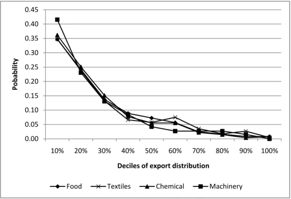
Figure 1, which comparesProb(Export Decilet|Entryt)across deciles, indicates that plants that

start exporting typically engage in small scale exporting operations. In all four industries, an over-whelming share of the new entrants begin their exporting operations at the bottom of the export distribution and the entry probability declines very fast across deciles of the export distribution: between 35 and 42 percent of new entries take place in thefirst decile of the export distribution,

between 60 and 65 percent take place in thefirst two deciles, while 80 to 90 percent take place below

the median of the export distribution. Figure 2, which comparesProb(Export Decilet−1|Exitt)

across deciles, shows that small exporters are far more likely to exit the export market. In all in-dustries, plants that exit are most likely to come from the bottom decile of the export distribution and the probability decreases very fast across deciles: 27 to 32 percent come from thefirst decile,

46 to 53 percent come from the first two deciles, while 75 to 82 percent of the plants that exit

had export sales smaller than the industry median. Both figures display a remarkable degree of

similarity across industries with respect to the entry and exit patterns.

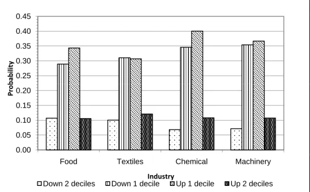
To describe the plant level dynamics of exporting activity at the intensive margin, we focus on plants that export in consecutive years and construct the matrix of year-to-year transitions between the deciles of the export distribution. Figure 3 plots the conditional probability of a plant changing its relative position in the distribution of exports (one minus the probability corresponding to the main diagonal of the transition matrix). The probability ranges between 20 and 90 percent and the graphs have an inverted-J shape, which indicates that top exporters have a very low probability of undergoing any change in their relative position, while plants in the middle of the export distribution have the highest mobility (60 to 80 percent will move either up or down in the

distribution of exports). Changes in plants’ relative position in the distribution of exports are not very dramatic. Figure 4 indicates that 60 to 75 percent of the moves take place between adjacent deciles while roughly 80 to 90 percent take place within two deciles, and that the percentages of plants that move up and down in the distribution of exports are similar.

These patterns of plant-level exporting dynamics suggest that exporting activity can be thought of as a ladder. Entries and exits take place into and from the bottom steps. Simultaneously, comparable shares of plants ascend and descend the exporting ladder, step by step. Both the upward and the downwardflows become increasingly sparse towards the top of the ladder; a small

fraction of plants reach the top and they are very likely to remain there.

3.3

Exporting dynamics and productivity performance

The intense and heterogeneous dynamics of exporting activity among plants that export in con-secutive years, on the one hand, and the fact that the vast majority of plants that enter and exit the export market are small exporters, on the other hand, suggest that exporting dynamics at the intensive margin accounts for a large share of the industry-level growth and plays an important role in explaining the relationship between exporting and productivity.

The matrix of year-to-year transitions into and out of the export market and across the deciles of the export distribution forms the basis for our study of the connection between plant-level dynamics of exporting activity and plant-level productivity performance. First, we distinguish between export dynamics at the extensive margin — plants that enter or exit the export market — and export dynamics at the intensive margin — plants that export in consecutive years and move down, move up, or do not change their relative position in the distribution of exports — and compare the relative importance of the contributions made by plants with different types of export

dynamics to thegrossindustry-level changes in exports, employment, output, and unweighted and weighted productivity. Second, we focus on plants that export in consecutive years and analyze the relationship between plant-level exporting dynamics at the intensive margin (move up, move down, or no change in relative position) and plant-level changes in productivity. Finally, for plants that move upwards in the distribution of exports we analyze whether becoming a large exporter is associated with larger gains in total factor productivity.

We construct the contributions of plants with different types of exporting dynamics to the gross

industry-level changes in exports, employment, output and unweighted and weighted productivity by adapting measures introduced by Davis and Haltiwanger (1999) for gross job creation and gross job destruction. We define the positive contribution of a subset A of an industry’s plants to gross

export change between t and t+ 1 as EXP_A+ = P i∈A+

∆EXPit and the negative contribution to

gross export change asEXP_A− = P i∈A−|

∆EXP_|it, whereiis an index for plants,A+_{is the subset of}

plants inAthat increase their export sales, whileA− _{is the subset of plants inAthat reduce their}

export sales betweentandt+ 1. We define in a similar way positive and negative contributions to

gross changes in employment output and weighted and unweighted productivity: - for employment, EM P_A+ = P i∈A+ ∆EM Pit and EM PA− = P i∈A−| ∆EM P_|it, whereA+ _{is the}

subset of plants in A that increase their employment, while A− _{is the subset of plants in A that}

reduce their employment betweentandt+ 1; - for output, OU T_A+ = P

i∈A+

∆OU Tit and OU TA− = P i∈A−|

∆OU T_|it, whereA+ _{is the subset of}

plants inAthat increase their output, whileA−_{is the subset of plants inAthat reduce their output}

betweent andt+ 1;

- for unweighted productivity, P RD_A+ = P i∈A+ ∆prit n and P RD − A = P i∈A− ¯ ¯ ¯ ¯∆prnit ¯ ¯ ¯ ¯, where A+ is

measure of their industry, whileA− _{is the subset of plants inAthat increase their contributions to}

the unweighted aggregate productivity measure of their industry betweentandt+ 1; - for weighted productivity , W P RD+_A = P

i∈A+

∆(sitprit) and W P RD−A = P i∈A−|

∆(sitprit)|,

whereA+ is the subset of plants inA that increase their contributions to the weighted aggregate

productivity measure of their industry, while A− _{is the subset of plants in A that increase their}

contributions to the weighted aggregate productivity measure of their industry betweentandt+ 1. In table 5 we present the contributions of plants that enter or exit the export market and of plants that continue to export to thegrossindustry-level changes in exports, employment, output, and unweighted and weighted productivity. With the exception of exports, the values do not add up to 100, the remainder representing the contribution of plants that sell exclusively on the domestic market. The results show that entries and exits account for much smaller shares of the positive and negative contributions to the gross changes in exports, employment, output, and weighted and unweighted total factor productivity than plants that export continuously. Entries in the export market account for 8.3 percent (in chemical) to 14.7 percent (in textile) of gross export growth, while exits from the export market account for 1.9 percent (in machinery) to 10.6 percent (in textile) of the negative gross export change. With respect to employment and output, contributions of exits and entries to both positive and negative gross changes represent one quarter or less of those made by plants that export continuously. Contributions of entries and exits to gross changes in the unweighted aggregate productivity measure of their industry represent 25 to 45 percent of those made by plants that export continuously. Finally, contributions made by entries and exits to gross changes in the weighted aggregate productivity measure of their industry represent 8 to 30 percent of those made by plants that export continuously, which implies that plants that enter and exit account for smaller shares of their industry output. A comparison across industries suggests that

in industries that export larger shares of the output (textiles, chemical, and especially machinery) plants that continue to export account for relatively larger shares of overall gross changes.

To study the relationship between the dynamics of plant-level exporting activity at the intensive margin and productivity performance, we focus on plants that export in consecutive years and define three types of exporting dynamics: ‘move down’ (plants that move into a lower decile of

the export distribution), ‘stay’ (plants that do not change their relative position in the distribution of exports, and ‘move up’ (plants that move into higher deciles of the export distribution. In column (1) of table 6 we present the results of linear regressions of changes in TFP as a function of the type of exporting dynamics. Coefficient estimates indicate that among plants that export

in consecutive years, there is a strong correlation between the dynamics of the exporting activity and the productivity performance. Plants that move down in the distribution of exports experience significant decline in total factor productivity (the constant terms are negative and significant in

all industries with magnitudes between -0.08 and -0.20). The coefficients for ‘stay’ and ‘move up’

are positive and significant in all industries and the F-tests show that in three of the four industries

(food, chemical, and machinery) the coefficients for ‘move up’ are significantly higher than those for

‘stay’. These results imply that plants that do not change their relative position in the distribution of exports experience very small changes in TFP — the sum of the constant term and the coefficient

for ‘stay’ is every close to 0 — while plants that move higher on the export ladder realize average total factor productivity gains of 0.05 to 0.13.

The relationship between plant-level exporting dynamics and average productivity performance is by no means the result of uniform gains (losses) by plants that intensify (reduce) their exporting activity. It is rather the aggregation of strongly heterogeneous plant behavior. We use kernel density estimation to construct the distribution of year-to-year changes in total factor productivity

for plants with different types of exporting dynamics. The four panels of figure 5 compare, by

industry, the distributions of TFP changes for plants that move downward in the distribution of exports, plants that do not change their relative position, and plants that move upwards in the distribution of exports. Among plants will all types of exporting dynamics there are both plants that realize TFP gains and plants that experience TFP losses. The distributions, however, are significantly different. For any level of TFP change, the probability of changes smaller than or

equal to that particular level (the cumulative distribution function, CDF) is largest for plants that move down in the export distribution and it is smallest for plants that move up in the export distribution.15

The fact that the distributions are significantly different is supported by the results of quantile

regressions, presented in columns (2) to (10) of table 6. Quantile regressions estimate the

coef-ficients of linear, conditional quantile functions in a way similar to that in which OLS estimates

the coefficients of linear conditional expectation functions. The interpretation of the coefficients is

also similar to that of coefficients in a linear regression: the partial derivatives of the conditional

quantile function with respect to the independent variables. For example, a positive coefficient for

an independent variable in the regression for 10th percentile indicates that a one unit increase in the independent variable will increase the 10th percentile of the distribution of the dependent variable by the value of the coefficient. We ran quantile regressions of change in the TFP as a function of

the type of export dynamics, by industry, for the 10th to the 90th quantiles. With very few excep-tions, the coefficients of ‘stay’ and ‘move up’ are positive and significant in all industries and for

all quantiles, which is consistent with the kernel density estimates showed infigure 5. The F-tests

1 5_{The distribution of TFP changes for plants that move down in the export distributionstochastically dominates}

the distributions of TFP changes for plants that do not change their relative position and for those that move up in the export distribution; the distribution of TFP changes for plants that do not change their relative position stochastically dominates the distribution of TFP changes for plants that move up in the export distribution.

indicate that the distribution of TFP changes for plants the move into higher deciles is significantly

different from that of plants that do not change their relative position in the export distribution.

These results imply that plants the move up in the distributin of exports are at the same time more likely to experience larger increases in their productivity and less likely to experience larger declines in theor productivity.than plants that do not change their relative position or move down in the distribution of exports.

We have showed that plants in the upper deciles of the export distribution are very different

from those in the lower deciles: they have much larger export volumes and higher export intensity. Focusing on plants that move upward in the export distribution, we assess whether becoming a large exporter is associated with relatively larger productivity growth. We classify year-to-year upward transitions in the export distribution with respect to their destination: transitions that end in the bottom 30 percent, the middle 40 percent, and the top 30 percent of the export distribution. We ran OLS and quantile regressions (for 10th to 90th percentiles) of changes in TFP as a function of the destination of the upward transitions. Table 7 shows the estimation results. The OLS estimates, presented in column (1) show that average TFP change for upward transitions that end in the bottom 30 percent of the export distribution are not significantly different from zero (for all

industries, the constant terms are not statistically significant). In three out of four industries (food,

chemical, and machinery) transitions that end in the middle 40 percent and those ending in the top 30 percent of the export distribution are associated with positive and significant average TFP

change. Moreover, in chemical and machinery industries, the F-tests for equality of the coefficients

for ‘middle 40%’ and ‘top 30%’ are significant, which indicates that in these industries, TFP growth

associated with becoming a large exporter is significantly higher.

the average TFP changes are generated primarily by differences at the bottom of the distribution.

In all industries the coefficients for ‘Top 30%’ (upward moves ending in the top 30 percent of

the export distribution) are positive and significant in the regressions for bottom (10th to 50th)

percentiles (columns (2) to (6)) and the coefficients of the lowest deciles are the largest. This shows

that low realizations of TFP change are significantly less likely for plants that move to the top of

the export distribution. In the machinery, the industry with the largest output and export and with the strongest concentration of exports, the coefficients for ‘Top 30%’ in the regressions for 8

of the 9 quantiles are significant, which indicates that that the largest TFP gains take place when

plants become large exporters.

4

Discussion

In this paper, we use panel data on Mexican manufacturing plants to study the relationship between plant-level dynamics of exporting activity and productivity performance. Our data contain informa-tion on plants from the four largest two-digit manufacturing industries and cover the period between 1993 and 2000, which encompasses the introduction of the North American Free Trade Agreement (NAFTA) in 1994, a severe macroeconomic crisis in 1995, and the temporary devaluation of the Mexican peso.

Our analysis has two main components. First, we analyze the plant-level dynamics of exporting activity. We show that exporting activity can be described as a ladder. Plants that export form a very heterogeneous group; within each industry, the top 10 percent exporters account for 54 to 90 percent of industry exports, have export salesfive to nine times the industry average, and have

significantly higher exporting intensity. Most entries into and exits from the export market take

while plants that exit are predominantly selected among small exporters. There is an intense dynamics of exporting activity at the intensive margin. Simultaneously, similar shares of plants move up and down the ladder, gradually changing their relative position in the distribution of exports. The mobility of plants across the distribution of exports has an inverted-J shape. Plants in the middle deciles of export distribution have the largest probability of changing their relative position, while the largest exporters have the lowest probability of changing their relative position. Second, we study the relationship between plant-level exporting dynamics and productivity per-formance. We distinguish between export dynamics at the extensive margin — plants that enter or exit the export market — and export dynamics at the intensive margin — plants that export in consecutive years and move down, move up, or do not change their relative position in the distrib-ution of exports. Entries and exits have relatively small contribdistrib-utions to gross, industry changes in all relevant variables — exports, employment, output, and productivity. Among plants that export in consecutive years, productivity performance is correlated with the type of exporting dynamics. Standard linear regression results show that improvements in plants’ relative position in the dis-tribution of exports are associated average total factor productivity gains, while deteriorations in plants’ relative position are associated with average total factor productivity losses. Kernel density estimation of the distribution of changes in TFP and quantile regressions show that the relationship between export dynamics and productivity is affected by a great deal of heterogeneity, but plants

that improve their relative position have superior distributions and becoming a large exporter is associated with larger gains in total factor productivity.

Our results are consistent with the predictions of theoretical models from two related strands of literature: models of exporting dynamics in industries with heterogeneous plants and sunk costs of exporting (Melitz, 2004, Helpman, Melitz, and Yeaple, 2004, Bernard, Eaton, Jensen, and Kortum,

2003) and models offirms’ dynamic employment and investment decisions under uncertainty, when

the adjustment costs of labor and capital are significant (Hammermesh and Pfann 1996, Bentolila

and Bertola, 1990, Dixit 1989, 1992, 1997).

Significant sunk costs of entering the export market create a range of inaction at the decisional

margin. Uncertainty about market conditions — either static, iffirms, for example, have imperfect

information about demand for their product until they enter the foreign market, or dynamic, if market conditions like demand or exchange rates are subject to random changes — widen the range of inaction. As a result, export responses to changes in the economic environment will be concentrated at current exporters. Existing exporters are in the best position to take advantage of improvements in the exporting conditions, while, on the other hand, they may prefer to incur temporary losses resulting from a decline in demand for their products rather than exit the foreign markets. In our sample, which covers the introduction of NAFTA and the temporary devaluation of the Mexican peso, exits into and entries from the export market account, roughly, for less than 10% of the gross changes in exports.

The ladder structure of the exporting activity, with new entrants starting at the bottom of the ladder and gradually advancing towards the top, suggests that plants incur not only a lump-sum cost of entering the export market, but also a convex-shaped, possibly piecewise linear, post-entry cost of adjusting their exporting activity. The cost that afirm incurs when expanding or contracting

their exporting activity has two sources: the pecuniary and non-pecuniary costs of adjusting labor — hiring, training, andfiring costs — and the costs of installing new capital or scrapping equipment and

the associated costs or reassigning and retraining the work force, as well as the irreversible character of some of the investments in capital. Standard results in dynamic labor demand (Hammermesh and Pfann, 1996) and investment theory (Dixit 1989, 1992, 1997) show thatfixed and linear adjustment

costs create a region of inaction for the decision to adjust the use of inputs, but if the value of the adjustment exceeds the cost, thefirms will immediately converge either to the optimal input levels

(in the cases offixed costs) or to levels determined by the limits of the range of inaction (in the case

of linear costs); convex costs, on the other hand, generate gradual adjustment paths towards the optimal levels of inputs. Accordingly,fixed or linear costs of adjusting the exporting activity would

imply that new exporters enter at their optimal level of exporting (or at the lower bound of the range of inaction). Subsequent adjustments would be triggered by unexpected changes in market conditions. If adjustment costs arefixed or linear, the fact that most of the entries and exits take

place at the bottom of the export ladder could be generated by plants’ having imperfect information about conditions in the foreign markets and engaging in small scale exporting operations to learn, for example, the demand for their product. Upon learning their demand, they may either decide to exit the market or further expand their exporting operations, directly to the optimal level. The gradual adjustment of exporting activity that we observe in our data, with a vast majority of plants that change their relative position in the distribution of exports moving to adjacent deciles, requires convex or piecewise-linear, convex adjustment costs.

Convex costs of adjusting the export levels also offer an explanation for the fact that mobility of

plants across the distribution of exports has an inverted-J shape, with the largest exporters being least likely to change their relative position. Plants in the tenth decile of the export distribution have export salesfive to nine times the industry average and three to twenty times the average export

sales of plants in the ninth decile. Becoming a large exporter implies sharp increases in export sales and large adjustment costs if these costs are convex. Only the most successful exporting plants can pay the high cost of becoming large exporters. Both the size of the adjustment costs of making it to the top of the export ladder, which widens the region of inaction, and the selection of most

productive plants reduce the mobility of large exporters.

The association wefind between the plant level dynamics of exporting activity and total factor

productivity growthfits well into this framework. If new entrants engage in small scale exporting

operations because of convex adjustment costs or imperfect information about demand in the foreign market, entries and exits will not be earth-shattering events in plants’ lives. The bulk of efficiency

enhancing actions that a plant takes in connection to its exporting activity will rather be associated with changes in the intensity of the exporting activity, mainly with becoming a large exporter. This result is consistent with previous empiricalfindings showing that while, on average, plants that enter

the export market at a given point in time do not outperform those that never export, plants that export for longer periods of time have a better performance than those than never export. Our study suggests, however, that this is not solely due to long term exporters being superior with respect to a time-invariant productivity parameter. It is rather the cumulative effect of plant heterogeneity and

significant post-entry productivity gains associated with the intensification of exporting activity.

Our results provide and explanation for the weak evidence of plant-level productivity gains from trade. Previous studies focused on the period before and immediately following entry into the export market, but, as we showed, entries take place at the bottom of the export ladder and are associated with relatively small TFP changes and very small output-weighted productivity changes; instead, the bulk of plant-level productivity gains from trade accrue long after entry when plants become large exporters.

References

Bentolila, S. and Bertola, G. (1990), “Firing Costs and Labor Demand: How Bad is Eurosclerosis?”

Review of Economic Studies 57, 381-402.

Bernard, A., Eaton, J., Jensen, J. B., and Kortum, S. (2003), "Plants and Productivity in Inter-national Trade,"American Economic Review 93, 1268-1290.

Bernard, A., Jensen, J. B. (1999), “Exceptional exporters performance: cause, effect or both?”

Journal of International Economics 47, 1-25.

Bernard, A., Jensen, J. B. (2004a), “Why Some Firms Export?” The Review of Economics and Statistics 86, 561-569.

Bernard, A. and Jensen, J.B. (2004b), "Entry, expansion and intensity in the U.S. export boom, 1987—1992,"Review of International Economics 12, 662—675.

Bernard, A., Jensen J. B, and Schott, P. K. (2006), ”Trade Costs, Firms, and Productivity”

Journal of Monetary Economics 53, 917-937.

Blalock , G. and Roy, S. (2007), "Afirm level examination of the exports puzzle why East-Asian

exports did not increase after 1997-1998financial crisis,"The World Economy 30, 39-59.

Bugamelli, M. and Infante L. (2002) "Sunk costs to exports," Bank of Italy Research Papers. Clerides, S., Lach, S. and Tybout, J. (1998), "Is learning by exporting important? Micro-dynamic

evidence from Columbia, Mexico and Morocco,"Quarterly Journal of Economics 113, 903— 948.

Davis S. J and Haltiwanger, J (1999), "Gross Job Flows," in Ashenfelter, O. and Card, D. eds,. Handbook of Labor Economics, vol 3B, 2711-2805.

Dixit, A.K. (1989), “Entry and Exit Decisions under Uncertainty,”Journal of Political Economy 97, 620 —638.

Dixit, A.K.(1992), “Investment and Hysteresis,”Journal of Economic Perspectives 6, 107-132.

Dixit, A. (1997), “Investment and Employment Dynamics in the Short-Run and the Long Run”

Oxford Economic Papers 49, 1-20.

Greenway, D. and Keller, K. (2007), "Firm Heterogeneity, Exporting and Foreign Direct Invest-ment,"The Economic Journal 117, 134-161.

Hammermesh, D. and Pfann, G. (1996), "Adjustment Costs in Factor Demand," Journal of Eco-nomic Literature 34, 1264-1292.

Helpman, E., Melitz, M. and Yeaple, S. (2004), "Export versus FDI,"American Economic Review 94, 300—316.

Lederman, D., Maloney, W., Serven, L. (2003), “Lessons form NAFTA for Latin American and Caribbean (LAC) Countries: A Summary of Research Findings," World Bank.

Levinsohn, J. and Petrin, A. (2003), “Estimating Production Functions Using Inputs to Control For Unobservables,”Review of Economic Studies 70, 317-341.

Lopez-Cordova, E. (2002), “NAFTA and Mexico’s Manufacturing Productivity: An Empirical In-vestigation Using Micro-level Data,” mimeo, Inter-American Development Bank, Washington, D.C.

Melitz, M. J. (2003), "The Impact of Trade on Intra-Industry Reallocations and Aggregate Indus-try Productivity,"Econometrica 71, 1695-1725.

Olley, S. and Pakes, A. (1996), “The Dynamics of Productivity in the Telecommunications equip-ment Industry,”Econometrica 64, 1363-1298.

Pavnick, N. (2002), “Trade Liberalization, Exit, and Productivity Improvements: Evidence from Chilean Plants,”Review of Economic Studies 69,245-276.

Roberts, M. J. and Tybout, J. R. (1997), "The Decision to Export in Colombia: An Empirical Model of Entry with Sunk Costs,"American Economic Review 87, 545-564.

Schiff, M. and Wang, Y. (2003), "Regional Integration and Technology Diffusion: The Case of

the North America Free Trade Agreement," World Bank Policy Research Working Paper No. 3132.

Tybout, J. R. (2003), "Plant and firm level evidence on new trade theories," in (E. Kwan Choi

and J. Harrigan, eds.), Handbook of International Economics, 388—415, Oxford: Blackwell.

Tybout, J. and Westbrook, M.D. (1995), “Trade Liberalization and the Dimensions of Efficiency

Appendix

A.1. Annual Industrial Survey

AIS uses a non-probabilistic sample drawn from the universe of manufacturing establishments provided by the 1993 Industrial Census. The sample was selected according to the following two cri-teria. First, two types of plants were excluded from the sample: establishments that operate under the special maquiladora regime and petrochemical and oil-refining plants which are state-owned

monopoly. Second, 205 six-digit industries with the largest contribution to total manufacturing production were selected from a total of 309 six-digit industries.16The largest plants from each in-dustry, covering at least 80% of the total value of gross production of the inin-dustry, were included in the sample. All remaining plants with at least 100 employees were added to the sample. In classes where production was highly concentrated, all establishments were included, whereas in classes with highly disaggregated production maximum 100 establishments were included in the sample. As a result, the AIS sample includes all the largest plants in the population and a significant share of

medium-scale plants, but a smaller share of small plants and very few micro-enterprises. The AIS sample has not been refreshed since 1993, but its composition changed every year. Plants were excluded from the sample for a number of reasons among which, plant closings are well identified.

Plants were added to the sample every year to replace the plants lost.

A.2. Imputation of capital stock

Capital stock is imputed using perpetual inventory method. The replacement value of capital stock provided by IC is the basis of the imputation procedure. Plants in the data set can be classified

in three categories: plants present in both IC 1993 and IC 1998, plants present in IC 1993 which 1 6_{Establishments are classified according to the Mexican Classification of Activities and Products, which at a}

exit the sample before 1998, and plants which enter the sample between 1993 and 1998, present only in IC 1998. For all plants which were in present in IC 1993 we impute capital stock using the replacement value of capital stock in IC 1993 as a basis. For plants which were present in both IC 1993 and IC 1998, we compare the imputed value of capital stock in 1998 with the value of capital stock in IC 1998 to obtain deflators for each of the seven types of capital stock. Finally, for plants

which initiated operations between 1993 and 1998, and were therefore present only in IC 1998, we impute capital stock by using the replacement value of capital in IC 1998, appropriately deflated,

as basis.

The second ingredient of the imputation procedure is the rate of depreciation of the capital stock. We use IC 1998 information on capital stock, investment, sales of capital, and depreciation to calculate depreciation rates forfive types of capital (excluding land), for 70five-digit manufacturing

sectors. For each firm we calculate depreciation rates for the five types of capital, then median

rates for each of thefive-digit sector are chosen. In calculating depreciation rates, it is important to

consider the distribution of investments and sales of capital during the year. The precise timing of the investments taking place during one year is generally not known and assumptions are necessary (for example, one can assume that all investments take place at the beginning of the year, at the end of the year or are uniformly distributed during the year). The assumed timing of the investments determines the denominator of the depreciation rate and, hence, the size of the depreciation rate. In this paper we assume both investments and sales of capital are uniformly distributed during the year.

Investments and sales of capital are the third ingredient of the imputation procedure. From AIS we extracted information on investments for two groups of capital stock types. First group pools together machinery, transportation equipment, computing and peripheral equipment, and furniture

and office equipment, the second group contains and buildings and land. Thefirst group is further

divided into domestic and imported capital goods. For each of these three types of investment we use deflators constructed by Banco de Mexico.

The perpetual inventory method is applied to each type of capital. The total capital stock is computed by summing the values for the six types and an imputed value of the rented buildings obtained by multiplying annual rent by 10. Capital stocks at the beginning and at the end of the year were calculated. In the estimation we use the average capital stock in a given year.

A.3. Estimation of the production function

We estimate industry-specific production functions using a modified version of the approach

introduced by Olley and Pakes (1996) in which the investment function is replaced by intermediate input demand. In this paper we use demand for electricity which, arguably, provides the best instrument since fewfirms produce electricity and electricity cannot be stored.

Consider the production function offirm at time t:

yit=α+βslsit+βuluit+βkkit+ωit+εit (1)

where yit is log value added, slits is log of skilled labor, luit is log of unskilled labor, kit is log of

plant’s capital stock,ωitis the level of plant specific productivity, andεit is white noise. A firm’s

private knowledge ofωit plays a role in both exit and input choice decisions. Firm’s demand for

electricity is:

Under monotonicity conditions, the demand function can be inverted,

ωit=ωit(eit, kit)

Replacingωit, (1) becomes:

yit=βslsit+βuluit+φ(eit, kit) +εit (2)

whereφ(eit, kit) =α+βkkit+ωit

In thefirst step we use OLS to estimate βˆ_s andβˆ_u in (2) where φ(eit, kit)is represented by a

polynomial expansion ineit andkit. Using the coefficient estimates at thefirst step, we calculate

an estimate forφ(eit, kit),ˆφ(eit, kit) =yit−βˆslsit−βˆulitu

Let

y_it∗₊₁=yit+1−βslsit+1−βulitu+1=α+βkkit+1+ωit+1+εit+1 (3)

To address the selection bias problem, firm’s exit decision is specifically modelled. Writing the

realization of the new productivity shock as a sum of a forecasted component and an idiosyncratic component, ωit+1 = E[ωit+1|ωit] + ηit+1,and denoting g(ωit) = α+E[ωit+1|ωit], equation 3

becomes

y∗

it+1=βkkit+1+g(ωit) +εit+1

exit decision is then represented by:

Xt = 1ifωt> ωt

Xt = 0otherwise

Incorporating the exit decision, (3) becomes:

y∗ it+1 = yit+1−βslits+1−βuluit+1= = α+β_kkit+1+E h ωit+1|ωit, ωt+1> ωt+1 i +η_it+1+εit+1

The second estimation step is then:

y∗_it+1=yit+1−βˆslits+1−βˆuluit+1=βkkit+1+g ³ ˆ φ(eit, kit)−βkkit,Pˆit ´ +η_it+1+εit+1 (4)

We use a polynomial expansion forg, g³φˆ(eit, kit)−βkkit,Pˆit ´ = P j P l β_jl³φˆ(eit, kit)−βkkit ´j ˆ Pl

it and non-linear least square to

estimate (4).

Finally, using the coefficient estimates from the two steps of the estimation, we calculate total

factor productivity as

ˆ

Figure 1. The destination of entries into the export market (yearly transitions). 0 25 0.30 0.35 0.40 0.45 ity 0 00 0.05 0.10 0.15 0.20 0.25 Pobabil 0.00 10% 20% 30% 40% 50% 60% 70% 80% 90% 100% Deciles of export distribution

Food Textiles Chemical Machinery

Figure 2. The source of exits from the export market (yearly transitions).

0.35 0.15 0.20 0.25 0.30 P obability 0.00 0.05 0.10 10% 20% 30% 40% 50% 60% 70% 80% 90% 100% P Deciles of export distribution

Figure 3. Conditional probabilities of changing relative position in the export distribution.  (yearly transitions) 0 5 0.6 0.7 0.8 0.9 lity 0 0 0.1 0.2 0.3 0.4 0.5 Pobabi 0.0 10% 20% 30% 40% 50% 60% 70% 80% 90% 100% Deciles of export distribution

Food Textiles Chemical Machinery

Figure 4. Plant mobility across the export distribution, by industry (yearly transitions).

0.25 0.30 0.35 0.40 0.45 b ability 0.00 0.05 0.10 0.15 0.20 Pro b

Figure 5. The distributions of changes in total factor productivity by industry and type of export dynamics

A. Food Products B. Textiles

1.2 1.4 1.2 1.4 0 2 0.4 0.6 0.8 1.0 1.2 Density 0 2 0.4 0.6 0.8 1.0 1.2 Density 0.0 0.2 -2.5 -1.5 -0.5 0.5 1.5 2.5 TFP Change

Move Down Stay Move Up

0.0 0.2

-2.5 -1.5 -0.5 0.5 1.5 2.5

TFP Change

Move Down Stay Move Up

C. Chemical D. Machinery

Move Down Stay Move Up Move Down Stay Move Up

0.8 1.0 1.2 1.4 1.6 nsity 0.8 1.0 1.2 1.4 1.6 nsity 0.0 0.2 0.4 0.6 -2.5 -1.5 -0.5 0.5 1.5 2.5 De TFP Ch 0.0 0.2 0.4 0.6 -2.5 -1.5 -0.5 0.5 1.5 2.5 De TFP Ch TFP Change TFP Change

Table 1. Estimates of production functions. Fixed effects estimation and semiparametric estimation

Sector

Coeff. S.E. Coeff. S.E Coeff. S.E Coeff. S.E. Coeff. S.E Coeff. S.E

(1) (2) (3) (4) (5) (6) (7) (8) (9) (10) (11) (12)

Food 0.231** 0.020 0.426** 0.027 0.241** 0.022 0.340** 0.048 0.294** 0.033 0.303** 0.031 Textiles 0.123** 0.020 0.603** 0.028 0.184** 0.025 0.352** 0.043 0.487** 0.030 0.307** 0.029 Chemical 0.206** 0.017 0.507** 0.023 0.229** 0.021 0.522** 0.036 0.137** 0.036 0.500** 0.031 Machinery 0.253** 0.015 0.685** 0.018 0.154** 0.017 0.475** 0.026 0.289** 0.025 0.402** 0.022

Note: **Significant at 95 percent level. *Significant at 90 percent level. Bootstrap standard errors are presented for semiparametric estimation

Fixed Effects Semiparametric Estimation