What factors affect the Oslo Stock Exchange?

(1)

What factors aect the Oslo Stock Exchange?

Randi Ns, Johannes A. Skjeltorp and Bernt Arne degaard

∗

November 2009

Abstract

This paper analyzes return patterns and determinants at the Oslo Stock Ex-change (OSE) in the period 1980{2006. We nd that a three-factor model con-taining the market, a size factor and a liquidity factor provides a reasonable t for the cross-section of Norwegian stock returns. As expected, oil prices signicantly aect cash ows of most industry sectors at the OSE. Oil is, however, not a priced risk factor in the Norwegian stock market. As the case in many other countries, we nd that macroeconomic variables aect stock prices, but since we nd only weak evidence of these variables being priced in the market, the most reasonable channel for these eects is through company cash ows.

JEL codes: G12; E44

Key Words: Stock Market Valuation, Asset Pricing, Factor Models, Generalized

Method of Moments

1 Introduction

In this paper we report results from an extensive empirical analysis of the Oslo Stock Exchange (OSE). The purpose of the analysis is to investigate whether the factors aecting the stock prices at the OSE can be explained using standard nancial theory, and to what extent the results from other stock markets are also found in the Norwegian stock market.

The theoretical and empirical asset pricing literature is internationally very exten-sive. In spite of this there are few analyses that specically study the Oslo Stock Exchange. The few extant studies are typically focused on the time series properties of

∗_{Ns and Skjeltorp are at Norges Bank. degaard is at the University of Stavanger and Norges Bank.}

Corresponding author: Johannes Skjeltorp, Norges Bank, Postboks 1179 Sentrum, NO-0107 Oslo,

Nor-way. Phone: +47 22 31 67 40. Fax: +47 22 42 40 62. Email: [email protected]

(2)

aggregate market returns. By leaving out information about return dierences across companies, and across time variation in company and sector weights, such analyses may give a misleading impression of the most important factors aecting the cross section of stock returns.1

The belief among participants in the Norwegian market seems to be that classical nance theory holds, for example that a company's market risk (beta) is important for the expected returns of a stock. There is, however, no in-depth test of whether the CAPM actually is able to price Norwegian stocks. Another \truth" among practitioners is that the OSE is driven by oil prices. Even if such a relationship seems probable, there is little empirical evidence to support this, and no clear understanding of how such a relationship is to be understood.

Knowledge of which risk factors are important for stock prices at the OSE, the magnitude of realized risk premia, and to what extent the cross-section of returns at the OSE is dierent from other stock markets is obviously of interest to investors on the exchange, and companies raising capital through the OSE. We nd that both level and variation of risk premia at the OSE have been high. Internationally, newer research suggests that variation in risk premia, both over time and in the cross-section, can be used to predict economic cycles. Improved understanding of the Norwegian stock market is therefore also important for government work on nancial stability and monetary policy.

1.1 Theories for pricing of equities

From investment theory we know that the value of a stock can be expressed as the present value of an uncertain future cash ow, where the discount factor is adjusted for risk. Similarly, the value of the OSE can be found as the present value of expected cash ows from all listed companies, discounted using a required rate of return reecting the risk of the cash ows. Mathematically, this can be expressed as

P₀M = n X i=1 ∞ X t=0 Et Di t+1 (1+rf t+1 +erit+1)t (1)

1_{Estimation using aggregate market returns typically nd what is important for the few largest}

companies/sectors in the market. This is particularly a problem when analyzing the Norwegian market, where a few companies account for a large part of the aggregate market value. Additionally one will not gain any understanding of factors aecting companies' earnings and risk in dierent sectors, and what factors aect all sectors.

(3)

where PM_t is the value of the market at time t, i indexes company, and there are n

companies listed on the exchange. Di

t is the cash ow of company i at timet and rft is

the risk-free interest rate at timet. Ifri

t is the return of companyi at timet, we dene

eri_t = (ri_t−rf_t) as the expected return in excess of the risk-free interest rate. This is the

necessary compensation for the uncertainty of cash ows for company i, i.e. the risk

premium. The present value formula shows that a factor which systematically aects the market return can do so through cash ows, risk-free interest rate, risk premia, or combinations of these. We typically distinguish between two channels: cash ow eects and risk premia. Cash ow eects inuence future cash ows of a company, and therefore future dividends Di_t₊₁. Risk premia will instead aect eri_t₊₁. Risk premia

are typically inuenced by systematic risk factors, which are common to all companies. An understanding of which of these two channels causes stock price changes will be an important part of the following analysis. Is, for example, a positive covariability between the market index and oil prices due to oil prices being a systematic risk factor aecting the required return for all companies, or is the eect mainly caused by changes in expected cash ows of oil and oil related companies?

Theoretical valuation models attempt to explain risk premia in the market. Com-mon to all models is the basic assumption of rational agents, and that prices (of equities and other nancial assets) are determined by the degree of covariability between the return of the assets, and the marginal benet of consumption. A company will typi-cally do well in some states and bad in other states, something which varies over time. Valuation models say that consumers value companies doing well in states and times when they have low wealth (low consumption) and therefore high marginal evaluation of an increase in wealth (consumption). This will increase prices (and thereby decrease returns) of these companies. On the other hand, the prices of companies doing well in good states or good times will be driven downward. These kinds of eects will, according to theory, generate the observed risk premia in the market.

The best known valuation model is the capital asset pricing model (CAPM). The CAPM explains returns on stocks by how sensitive the company is to the return on a portfolio containing all wealth in the economy (the market portfolio). The CAPM is usually specied in an unconditional framework as

(4)

where E[ri] −rf is the expected risk premium for company i, E[rm] −rf is the expected

risk premium for the market, andβi

m measures the covariability between the return on

stocki and the market portfolio.2 If we set eri=E[ri] −rf, and letλm =E[rm] −rf be

the market risk premium, we observe that the CAPM may also be expressed as

E[eri] =λmβim, (2)

whereE[eri] is the expected return on companyiin excess of the risk-free rate, and λm

is the risk premium of a unit market risk. The CAPM formalizes in a simple manner the idea that the expected return on an asset should be increasing with the risk of an asset.3 _{The model is, however, based on very simplied assumptions, among them that}

the economy only lasts for one period. Currently it is therefore more common to use the intertemporal CAPM or the Arbitrage Pricing Theory (APT) as theoretical bases for estimation. Unconditionally, both the ICAPM and the APT can be expressed as

E[eri] =

X

j

λjβij, (3)

whereβi

j is companyi's exposure to risk factorjandλjthe risk premium linked to factor

j. The ICAPM is an expanded version of the CAPM where investors with longer

in-vestment horizons want to hedge future reinin-vestment risks.4 _{This is modelled through}

state variables aecting investors' optimization problem over consumption and asset portfolios. State variables which predict market returns and changing investment op-portunities are risk factors pricing companies. This is the extent to which the ICAPM species state variables; they are not linked directly to observable and measurable eco-nomic variables. Wealth/income is, however, an obvious candidate for a state variable. Assets covarying positively with wealth will in such a model have relatively low prices and high expected returns, because investors demand compensation for investing in assets with low returns in periods/states with low wealth (where the marginal utility of income is high). In addition there are variables or news which aect investors future consumption opportunities. Often suggested variables in such settings are GDP and

2_{In an unconditional framework one assumes that risk premia are constant over time.}

3_{Investors demand risk compensation to invest in companies which fall in value at the same time as}

the market falls. The price of low-beta stocks increases and the price of high-beta stock decreases until the consumer's marginal utility of one unit of consumption is equalized across states.

4_{The following description of the ICAPM and APT are based on chapter 9 in Cochrane (2005), to}

(5)

ination.5 _{The model was developed by Merton (1973). At the time there was little}

belief in the existence of variables capable of predicting returns. Accumulated empirical evidence in the following 30 years has, however, identied some predictability in stock returns. As a result the ICAPM has seen a renaissance in recent years.

The APT model was developed by Ross (1976). The model takes as a starting point empirical observations of stock price evolutions. In good times, when the market increases, most stocks also increase. Similarly, there are obvious common components of the stock evolution in an industry or sector. Ross shows how, from a purely statistical characterization of the realized stock return, and simple arbitrage arguments, one can show that expected returns will be characterized by a multi-factor model of the type specied in (3).

The dierence between ICAPM and the APT model is primarily the motivation behind the chosen factors. In the APT one nds common factors through statistical analysis of realized returns, while in the ICAPM the focus is on state variables capable of describing the contingent distribution of future returns. The empirical implementation of both of these theoretical models will be the same; empirically it is therefore not important which model is used as a basis for the factors incorporated in the regressions. In newer nance literature it is common to express all asset price models in a general framework typically expressed as

Pi,t=Et[mt+1xi,t+1] (4)

where Pi,t is the price of an asset i at time t, xi,t+1 is the future cash ow from the

asset, and mt+1 the marginal utility of wealth (also termed the intertemporal rate of

substitution, the stochastic discount factor (SDF) or pricing kernel).

Dierent valuation models result in dierent specications of m. Independent of

model, however, it is natural to interpretm as a countercyclical variable which is large

in bad times and small in good times. As we will see this general framework is useful when interpreting relations between the stock market and macroeconomic variables. The framework in (4) is also the starting point for the currently most common way of empirically testing valuation models. Let us also remark that all of the models we have discussed earlier may be interpreted as special cases of this framework. If we, for

5_{In equilibrium all investors will invest in a portfolio of a risk-free asset, the market portfolio, and}

(6)

example, let m be a function of only the market portfolio, we are back in a CAPM

world.6

1.2 Summary of main results

Our study is based on a data-set including all stocks listed on the Oslo Stock Exchange (OSE) in the period 1980 to 2006. In section 2 we survey some important character-istics of the development of the exchange through the period. In section 3 we rst describe relations between stock returns and various empirical regularities also found in other stock markets, such as the size, book-to-market and momentum eects. We then proceed to construct risk factors using these eects and test the CAPM against various dierent empirically motivated multi-factor models. We also discuss dierent explanations of the empirical risk factors. Finally, we test dierent multi-factor models based on macro variables.

The main results from our analysis is that the return at the OSE can be explained reasonably well by a multi-factor model consisting of the market index, a size index, and a liquidity index. As expected, changes in the oil price aects the cash ows of most industry sectors at the exchange. Oil is however not a priced risk factor in the Norwegian market. As found in various other markets, there are few macrovariables priced in the market. We do however document a few signicant risk premia for the variables ination, money stock, industrial production and unemployment when we attempt to price portfolios sorted on size and liquidity. We nd a signicant relation-ship between most industry portfolios and the nominal variables ination and money stock; portfolio returns fall with unexpected increases in ination and increase with unexpected increases in money stock. Since we nd little signs of these variables being priced in the market, it is reasonable to believe that the main eect on returns from these variables is through the companies' cash ows.

6_{All valuation models can be written in excess return form as} _E_[_er_i_{] = −}_r_f_cov₍_m_{, er}_i₎ _{where the}

specic valuation model (erm in the CAPM version) is replaced bym. The expression says the same as

the CAPM, only with the opposite sign. Companies with a positive covariation with m (i.e. give high

returns when consumers put a high value on consumption), have a lower expected return (higher price). In the same way the traditional discounted value expression in (1) can be written as

pi₀= ∞ X t=0 Et _D i,t+1 1+rf−rfcov(m, eri) . (5)

(7)

2 The Oslo Stock Exchange 1980-2006

Our analysis of the Norwegian equity market uses monthly returns for all stocks listed on the OSE in the period 1980{2006.7 _{In this section we survey some of the important}

features of the development of the exchange in the period.

2.1 Organization of the market

The OSE has made a number of changes to its market structure in the period. In 1988 the earlier call auction was replaced with an electronic platform. The new system allowed for continuous trade throughout the day. The introduction of a new trading system (ASTS) in 1999 allowed for trade through the Internet. A number of specialized Internet brokers were established at the time. In 2000 the OSE joined the NOREX alliance, comprising all Nordic and Baltic exchanges.8 _{The purpose of the alliance was}

to create a common Nordic/Baltic platform for the exchanges and market participants to compete as simply as possible. As part of the alliance the dierent NOREX exchanges have to some degree harmonized their regulations. All the major exchanges are using the same trading platform, allowing investors access to the Nordic investment universe from one trading terminal. The OSE moved to the common platform with the other NOREX exchanges in 2002 (SAXESS). Everyone wanting to trade stocks using SAXESS has to go through an authorized broker. Such authorized brokers are called exchange members (brsmedlem). The trading system gives the exchange members access to an electronic limit order book for each stock. Supply and demand for stocks is registered in the limit order book, and trades are executed automatically when price, volume, and other order characteristics coincide. SAXESS updates continuously all changes in the market and oers real-time distribution of information to the members. In 2006 the opening hours for the OSE were increased to match the international market for equities.

7_{Accounting, price and volume data are from the OSE data service (Oslo Brsinfomasjon (OBI)).}

8_{The NOREX alliance comprises the exchanges in Oslo, Stockholm, Helsinki, Copenhagen, Reykjavik,}

(8)

2.2 Sectors

We use the GICS standard to group the companies on the OSE.9 _{GICS contains 10}

industry sectors. A company is put into a GICS category based on its most important business activity. The most important activity is usually decided based on sales. The ten major GICS industries are listed in table 1.

Table 1 The GICS standard

10 Energy and consumption 15 Materials/labor 20 Industrials 25 Consumer Discretionary 30 Consumer Staples 35 Health Care/liability 40 Financials

45 Information Technology (IT) 50 Telecommunication Services 55 Utilities

The energy sector comprises all the oil companies. The sector materials comprises such industries as chemicals, building materials, wrappings, mining, metals, paper and pulp. Utilities comprises companies in power, gas and water supplies as well as independent power producers and buyers.

2.3 Market size and activity

The OSE has been growing steadily over the period 1980{2006 both measured in trading volume and values. This is illustrated in gure 1, which shows the monthly development of respectively total trading volume and total market values for all listed companies. Tables 2 and 4 show the development of market sizes distributed on industry sectors, measured in respectively number of companies and market values.

In 1980 the 93 listed companies on the Oslo Stock Exchange had a total market value of NOK 16,500 million. At the end of 2006 the exchange had 253 listed companies and a total market value about NOK 1.95 billion. The average market value also increased in the period from 170 million in 1980 to 7,510 million in 2006. From 1998 to 2004 the number of listed companies fell from 269 to 207, mainly due to a reduction in the number of industrials. In 2002 the market weight of industrials fell from 23 % to 9 %.

9_{The GICS standard (Global Industry Classication Standard) was developed by Morgan Stanley}

Capital International (MSCI) and Standard & Poors (S&P). For companies that were delisted before 1997 there is no ocial OSE classication. We have therefore manually reconstructed the classication

(9)

Figure 1 Total market value and trading volume - OSE 1980-2008

The gures show the development in activity at the OSE over the period 1980 to 2009:6 measured by monthly market values (left) and monthly total trading volume (right) for all listed companies

0 0.5 1 1.5 2 2.5 1979 1982 1985 1988 1991 1994 1997 2000 2003 2006 2009 2012 Total Market Value OSE(bill)

0 50000 100000 150000 200000 250000 300000 350000 1979 1982 1985 1988 1991 1994 1997 2000 2003 2006 2009 2012 Monthly trade volume (mill)

This was due to a reclassication of one large company, Norsk Hydro, from industry to energy.

Companies on the OSE are concentrated in a few sectors. Up to 1990 the two dominating sectors were Industrials and Financials. In terms of number of companies this pattern has changed over the last 15 years due to an increase in the IT sector and decrease in the industry sector. Looking instead at market weights for each industry sector this pattern is somewhat modied. We observe that the IT sector has a relatively low weight even though almost 20 % of the companies were in this sector in 2006. The energy sector has had a marked increase in market weights the last years, from 10 % in 2000 to 50 % in 2006. This is due to the listing of Statoil, the state oil company, and the reclassication of Norsk Hydro in 2002. Some sectors only comprise a few companies. Utilities and telecommunications were hardly present at the OSE until the mid-nineties.

A prominent characteristic of the OSE is that the exchange always has a few very large companies, companies that dominate the value of the exchange. To illustrate this we include gure 2, which shows the fractions of the value of the exchange in the largest companies. In 2006 the three large state-dominated companies Statoil, Norsk Hydro and Telenor accounted for more than 53 % of the total market value of the OSE.

In table 3 we show average market values for companies in the various sectors, for the whole period and for three subperiods. The industrial sector had the largest companies until the last subperiod, when the energy sector, dominated by oil companies, took

(10)

Table 2 The number of companies listed on the Oslo Stock Exchange for the period

1980-2006

The table shows the number of listed companies on the Oslo Stock Exchange over the period 1980 to 2006 distributed on industry sectors. Note that the table shows the number of companies and not securities. A number of companies have more than one security issued.

Year Total Industry sector (GICS)

10 15 20 25 30 35 40 45 50 55 1980 93 9 10 28 6 9 1 28 2 -1981 96 9 11 28 7 9 1 29 2 -1982 109 12 12 30 12 9 1 30 3 -1983 120 12 11 36 13 9 2 31 6 -1984 138 14 12 42 15 10 2 36 7 -1985 158 17 12 48 18 11 2 37 13 -1986 165 18 12 51 18 11 2 39 13 1 -1987 159 20 12 47 15 9 2 39 13 2 -1988 144 19 11 45 13 7 2 33 12 2 -1989 141 17 11 44 11 7 2 37 12 -1990 142 20 9 46 10 7 2 37 11 -1991 131 21 9 45 9 5 2 30 10 -1992 134 20 9 46 14 3 2 30 10 -1993 145 19 9 55 17 4 2 29 10 -1994 156 19 10 60 18 3 3 32 11 -1995 173 20 11 63 21 2 3 39 14 -1996 186 24 12 60 22 3 3 39 21 1 1 1997 226 37 13 71 25 5 5 39 29 1 1 1998 243 36 12 75 28 6 5 45 34 1 1 1999 245 33 11 72 28 6 6 47 39 2 1 2000 246 34 13 60 25 6 7 48 49 3 1 2001 231 36 9 57 22 8 7 45 44 2 1 2002 219 36 9 48 20 9 7 44 43 2 1 2003 209 37 8 41 21 8 8 42 40 2 2 2004 203 35 9 40 18 9 10 38 41 1 2 2005 237 53 9 42 17 13 11 43 46 1 2 2006 253 62 10 44 19 14 13 40 47 2 2

(11)

Figure 2 The largest companies on the Oslo Stock Exchange 0 10 20 30 40 50 60 1979 1982 1985 1988 1991 1994 1997 2000 2003 2006 2009 Norsk Hydro

Statoil TelenorSaga Hafslund

Table 3 Market value of companies in dierent industry sectors.

The table shows the average market value of companies within the dierent GICS sectors for the period 1980-2006 and three sub-periods; 1980-89, 1990-99 and 2000-2006.

Average market value for industries (bill. NOK)

10 15 20 25 30 35 40 45 50 55 Whole period 1980-2006 20.75 6.99 31.46 6.15 7.49 5.65 17.52 5.36 2.86 0.38 Sub-periods 1980-1989 9.88 10.43 39.39 4.06 6.92 4.08 21.86 6.60 0.04 0.00 1990-1999 19.36 5.99 35.94 7.43 8.85 7.11 15.57 3.82 0.79 0.39 2000-2006 38.26 3.51 13.73 7.29 6.37 5.80 14.10 5.78 9.84 0.93

(12)

From 1980 to 2006 the annual trading volume on the OSE increased from about NOK 370 million to about NOK 2.6 billion. In other words, currently one day of trading is larger that half a year of trading 26 years ago. The liquidity has also signicantly improved. On average the number of trading days per stock has increased from 48 days in 1980 to 181 days in 2006.

Finally, to illustrate the importance of the OSE in the Norwegian economy we show in gure 3 the market value of all stocks on the exchange relative to annual Gross Domestic Product (GDP). In 1980 the market value of all stocks on the OSE was 5 % of annual GDP, a number which has increased to 90 % in 2006.

Figure 3 The market value of the Oslo Stock Exchange relative to GDP (percent)

The gure shows yearly development in the marketvalue of all companies listed on the Oslo Stock Exchange as a percent of GDP. The GDP gures are obtained from Statistics Norway (SSB).

0 20 40 60 80 100 120 1979 1982 1985 1988 1991 1994 1997 2000 2003 2006 2009 2012

Market value OSE as fraction of GDP(percent)

2.4 Stock returns

As a nal part of our descriptive analysis of the OSE we look at stock returns. Panel A in table 5 shows the average monthly return for industry portfolios, while panel B in the same table shows correlations between monthly returns of sector portfolios. In terms of average returns the IT and Energy sectors have been the most protable over the period 1980{2006. The same sectors have also been the most risky, measured

(13)

Table 4 Market value of listed companies on the Oslo Stock Exchange for the period

1980-2006.

The table shows the total and average market value of companies listed on the Oslo Stock Exchange for the period 1980-2009:6. The table also shows the market capitalization weights for the 10 GICS industry sectors and the weight of the four largest companies during the period.

Market value weight in % Year Total average for industry sector (GICS)

(bill. NOK) (bill. NOK) 10 15 20 25 30 35 40 45 50 55

1980 16.5 0.17 11 9 58 1 2 1 18 1 -1981 17.7 0.18 10 9 51 2 5 1 24 4 -1982 17.0 0.15 8 8 39 3 5 2 28 6 -1983 38.3 0.31 9 10 37 2 5 3 22 12 -1984 51.5 0.36 9 11 31 4 7 3 23 12 -1985 77.2 0.47 8 11 31 6 7 5 22 11 -1986 77.7 0.45 7 11 34 8 10 4 24 10 0 -1987 72.6 0.42 10 12 31 7 12 6 27 6 0 -1988 102.2 0.65 10 10 43 5 8 9 15 3 0 -1989 166.9 0.95 16 12 40 3 9 6 17 2 -1990 156.3 0.84 21 8 40 3 10 7 16 2 -1991 133.8 0.78 24 7 42 3 12 12 9 2 -1992 115.1 0.68 19 6 41 5 15 12 9 2 -1993 215.5 1.17 18 8 37 6 12 5 16 2 -1994 254.3 1.30 16 8 41 6 6 5 18 1 -1995 289.9 1.49 16 7 38 6 6 6 20 4 -1996 404.5 1.96 24 5 36 6 7 3 18 5 1 1 1997 614.2 2.46 25 3 29 10 6 9 15 5 1 1 1998 460.9 1.71 15 4 27 15 6 7 18 5 2 1 1999 619.2 2.35 16 5 28 16 6 6 17 11 4 1 2000 701.9 2.71 10 5 27 10 8 8 17 11 13 1 2001 755.8 3.06 25 4 23 6 6 8 15 7 9 1 2002 562.8 2.49 43 4 9 6 7 8 15 4 9 1 2003 784.3 3.60 43 4 6 8 5 9 16 4 10 1 2004 986.9 4.77 43 3 10 9 6 8 14 4 10 1 2005 1456.8 6.07 53 3 11 6 6 0 11 4 8 1 2006 1952.7 7.51 50 2 10 5 6 0 11 6 10 1

(14)

by the standard deviation of the return. The returns of sector portfolios are highly correlated. The largest correlation we nd for the energy and industry portfolios, with a correlation of 73 %.

Table 5 Historical returns for industry sectors (GICS)

Panel A shows the average equally weighted return for industry portfolios based on the GICS classi-cation. For each portfolio, the table shows the rst and last year for the return calculation, average monthly return (in percent), the standard deviation, the average number of companies in each portfolio and the number of months used in the calculation. Panel B shows the correlations between the monthly returns for the industry portfolios.

Panel A: Monthly return on industry portfolios

First Last Mean Standard- Average Number year year return deviation companies obs

Energy 1980 2007 2.53 9.74 19.6 336 Materials 1980 2007 1.93 8.62 7.6 336 Industrials 1980 2007 2.03 6.26 32.4 336 Consumer Discretionary 1980 2007 1.72 6.87 12.1 336 Consumer Staples 1980 2007 2.08 6.54 6.9 336 Health Care/liability 1980 2007 1.85 9.64 3.9 336 Financials 1980 2007 1.40 5.14 28.6 336 Information Technology 1980 2007 2.65 11.63 12.2 336 Telecommunication Services 1987 2007 1.12 11.46 1.3 152 Utilities 1996 2007 1.41 6.80 2.4 144

Panel B: Correlation between industry portfolios

Energy Materials Industrials Discr. Staples Health Financ. IT Telecom Materials 0.55 Industrials 0.73 0.64 Discr. 0.50 0.52 0.63 Staples 0.55 0.52 0.59 0.52 Health 0.39 0.36 0.45 0.40 0.35 Finan. 0.62 0.58 0.68 0.62 0.59 0.35 IT 0.53 0.36 0.49 0.47 0.46 0.47 0.45 Telecom. 0.37 0.24 0.36 0.40 0.28 0.49 0.38 0.56 Utilities 0.32 0.20 0.44 0.24 0.40 0.21 0.38 0.32 0.25

(15)

3 Empirical analysis of factors affecting returns

The rst formalized model for pricing of nancial assets was the Capital Asset Pric-ing Model (CAPM). The CAPM was developed by Sharpe (1964), Lintner (1965) and Mossin (1966) in the mid-sixties. By expanding the model to also account for reinvest-ment risk Merton (1973) extended the CAPM to the multi-factor model ICAPM. A few years later another multi-factor model (APT) was developed by Ross (1976). The CAPM was, however, the most used model for investigating risk and expected return till the beginning of the nineties.

During the eighties academics discovered a number of empirical regularities in stock returns which were not compatible with the CAPM. For example, one found that large companies on average had a lower return than small companies, even after adjusting for market risk. Since such observations were not compatible with the theory, they were termed \anomalies." In an important article Fama and French (1993) show that an empirically motivated multi-factor model, based on market risk and two of the anomalies had better explanatory power than the CAPM alone. In addition, one found in several empirical investigations support for predictability of stock returns on medium term horizons. Together these empirical results led to a renaissance of the multi-factor models developed in the seventies.

Estimation of multi-factor models can be grouped in two categories. One group constructs risk factors based on the anomalies relative to the CAPM. Such studies have met with considerable success in explaining stock returns, but they do not improve our identication and understanding of the underlying factors aecting returns. Some studies have, however, succeeded in relating the empirically motivated risk factors to underlying macroeconomic relations, such as business cycle and default risk. The other group investigates the link between realized stock returns and macroeconomic variables directly.

In this section we investigate what model specications are best suited to explaining returns at the OSE from 1980 to 2006. We start by investigating the importance of anomalies in the Norwegian stock market by a few simple portfolio sorts. We then go through our chosen estimation methods, before presenting results for estimation of the CAPM on portfolios sorted by market risk, industries, and the various anomalies. We then present results from estimations of multi-factor models based on the empirically motivated risk factors, and summarize the literature which attempts to nd the

(16)

under-lying factors behind the empirical factors. Finally, we present results from estimations using multi-factor models on macro variables.

3.1 Simple portfolio sorts based on CAPM anomalies

The three CAPM anomalies { rm size, book value relative to market value (B/M) and return momentum { were discovered in the US stock market. The anomalies have however shown remarkable persistence across markets and over time. A fourth char-acteristic often related to CAPM anomalies is liquidity. In this section we investigate, using portfolio sorts, whether these four characteristics also seem relevant for returns in the Norwegian market. In subsection 3.4 we perform a formal test of the relationship between CAPM anomalies and risk-adjusted returns. We also go through the literature attempting to explain why these characteristics are relevant for returns.

3.1.1 Company size

The size eect is an empirical regularity showing that investments in small companies on average have had a (risk-adjusted) return premium relative to investments in small companies. The size eect was rst documented using US data 1936-1975 by Banz (1981). After Banz's study the size eect has been documented in similar studies in 17 other countries, which according to Dimson and Marsh (1999) make the size eect the most documented stock market anomaly in the world. The size eect has however turned out to be very sensitive to choice of time period. For most countries the eect was negative in the period 1980{2000, that is the twenty-year period after Banz's publication of his results. Over the short period from 2000 it has again become on average positive.

To investigate the size eect in Norway we use a portfolio sort method where we construct portfolios based on companies' market values at the end of the previous year. The portfolio compositions are xed throughout the year, and re-balanced at the end of the year. Basing the portfolios on ex ante characteristics guarantees that this is an implementable trading strategy. Note however that the method does not adjust for risk dierences.

Table 6 shows excess returns (returns in excess of the risk-free rate) for 10 portfolios sorted on size for the period 1980-2006. Portfolio 1 contains the smallest companies and portfolio 10 the largest companies. Table 6 shows a positive dierential return

(17)

in the period: The smallest companies have had the highest returns, and returns are falling almost monotonically with size. The period average dierential return between a portfolio of the smallest companies and the largest companies has been more than 2% per month. We seem to have had a size eect also in the Norwegian stock market. An interesting observation is that the size eect seems to have been positive over a period when it was negative in other countries. In panel B of the table we observe that the dierential return between small and large companies has been positive also for subperiods, but has fallen over time. The last column of the table shows the results for a test of whether the dierential return between the two portfolios is signicantly dierent from zero. For the last subperiod (2000-2006) we do not nd support for a signicant dierence in the returns of small and large companies.

Table 6 Monthly excess returns for portfolios sorted on company value

Panel A shows the monthly percentage excess returns for 10 portfolios constructed based on market value. The results are for the whole sample period 1980-2006. The portfolios are re-balanced at the end of each year. Panel B shows the average monthly return for the portfolio containing the 10% smallest rms (portfolio 1) and the 10% largest rms (portfolio 10) on the exchange for three sub-periods. The table also show t-values from a test of whether the return dierence between the portfolios is zero.

Panel A: Whole sample 1980-2006

Excess return Number of stocks

Portf. Mean (std.dev.) min median max min median max

1 2.66 (7.9) -19.0 1.59 45.5 4 12 18 2 1.94 (7.1) -18.8 1.77 31.1 3 12 18 3 1.08 (7.2) -23.9 0.97 32.3 3 12 18 4 1.12 (7.2) -24.6 1.10 26.1 3 12 18 5 1.42 (7.2) -15.8 1.03 52.5 3 12 17 6 1.16 (6.7) -30.4 1.15 26.9 4 13 18 7 0.87 (7.4) -25.3 0.86 47.0 3 12 18 8 0.80 (7.0) -24.9 0.95 18.8 3 12 18 9 0.69 (8.0) -29.7 0.96 22.4 3 12 18 10 0.44 (7.1) -30.2 0.70 24.2 3 12 17 Panel B: Sub-periods

Small Large t-test

(Portf.1) (Portf.10) Di. di=0

1980-1989 8.14 1.80 6.34 4.48

1990-1999 4.51 1.50 3.01 3.66

(18)

3.1.2 Book value relative to market value

Another company characteristic which seems to give a systematic pattern in returns across companies is the relationship between book values and market values. Several studies, for example Rosenberg, Reid, and Lanstein (1984), Fama and French (1992) and Lakonishok, Shleifer, and Vishny (1994), nd that companies with the highest book values relative to market values have systematically higher risk-adjusted returns than those with the lowest book value relative to market value.

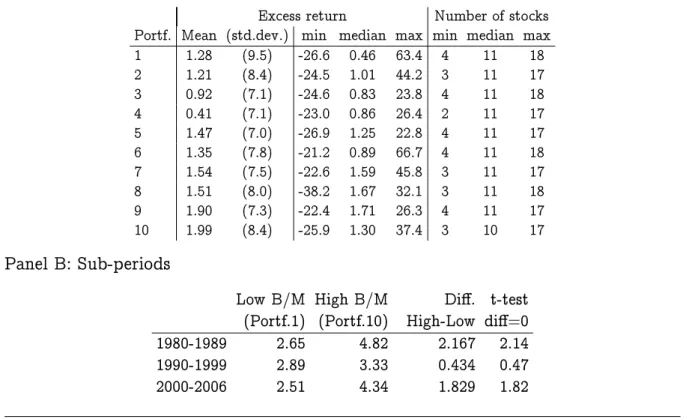
To investigate whether there are any systematic return dierences between compa-nies based on dierences in B/M ratios in the Norwegian stock market we construct portfolios in a similar manner to the size portfolios. Table 7 shows the results from this analysis. Portfolio 1 (10) contains the companies with the lowest (highest) B/M ratio. Portfolio 10 gives on average a (not risk-adjusted) excess return of 0.7 % per month compared with portfolio 1. It is substantially below the dierences due to company size. Also note that the relationship between B/M and return is much less systematic than that due to size. In the table's panel B we show returns for the two extreme portfolios based on B/M for three subperiods. We see that the B/M eect has been dominating in the rst part of the period, and the the return dierence is not signicant for the last two subperiods.

3.1.3 Momentum

Jegadeesh and Titman (1993) document that an investment strategy dened as buying stocks with high returns the last 3-12 months and selling companies with a low return over the same periods (buying winners and selling losers) give a risk-adjusted excess return.10 _{The strategy, which is called momentum, was already known and commonly}

used by portfolio managers.11

Momentum strategies have also been shown to work outside the US. Rouwenhorst (1998) documents momentum strategies in 12 European stock markets over the period 1980{95, while Chan, Hameed, and Tong (2000) nd support for momentum strategies in 23 international stock indices, of which 9 Asian, 11 European, two North-American and one South-African.12

10_{Jegadeesh and Titman (1993) use data from the US market over the period 1965 to 1989. Jegadeesh}

and Titman (2001b) show that momentum strategies also worked in the nineties.

11_{See Jegadeesh and Titman (2001a) for a survey of the American literature.}

(19)

Table 7 Monthly excess returns on portfolios sorted on B/M

Panel A shows the monthly percentage excess returns for 10 portfolios constructed based on Book to Market value (B/M). The results are for the whole sample period 1980-2006. The portfolios are re-balanced at the end of each year. Panel B shows the average monthly return for the portfolio containing the 10% rms with the lowest B/M-value (portfolio 1) and the 10% of the rms with the highest B/M-value (portfolio 10) for three sub-periods. The table also show t-values from a test of whether the return dierence between the portfolios is zero.

Low B/M High B/M Di. t-test

(Portf.1) (Portf.10) High-Low di=0

1980-1989 2.65 4.82 2.167 2.14

1990-1999 2.89 3.33 0.434 0.47

(20)

Table 8 shows monthly returns of portfolios sorted on momentum in the Norwegian stock market. Portfolio 1 contains the stocks with the lowest return the previous 11 months, while portfolio 10 contains stocks with the highest return. The dierential return between portfolio 10 and portfolio 1 was on average 0.44 % per month. The return dierences are however not monotone in momentum. Also for subperiods we see in panel B little support for a signicant momentum eect. The dierential return also changes sign in the second sub-period.

Table 8 Monthly excess returns for portfolios based on momentum

Panel A shows the monthly percentage excess returns for 10 portfolios constructed based on momentum. The results are for the whole sample period 1980-2006. Momentum is dened as the return from January until the portfolios are re-balanced at the end of the year. Thus, portfolio 1 contains the rms with the lowest return the previous year, and portfolio 10 contains the rms with the highest previous year return. Panel B shows the average monthly return for the portfolio containing the 10% of the rms with the lowest previous year return (portfolio 1) and the 10% of the rms with the highest previous year return (portfolio 10) on the exchange for three sub-periods. The table also show t-values from a test of whether the return dierence between the portfolios is zero.

Low MOM High MOM Di. t-test

1980-1989 2.51 4.18 1.666 1.84

1990-1999 3.72 1.97 -1.756 -1.96

2000-2006 2.48 3.50 1.021 0.86

3.1.4 Liquidity (transaction costs)

One characteristic often related to CAPM anomalies is liquidity. Level and variation in companies' liquidity has been suggested as explanations of the size eect, B/M eect and momentum eect, see for example Acharya and Pedersen (2005), Liu (2006) and

(21)

Sadka (2006). These results suggest that the observed anomalies in returns both across companies and over time may be a result of unrealistic assumptions in the CAPM development of static and frictionless markets.13

A problem with the concept of liquidity is that it has several dimensions: a cost dimension (how much it costs to trade), a time dimension (how fast one can trade), and a quantity dimension (how much one can trade). This has led to a proliferation of liquidity measures in the literature, with little agreement about which to prefer.

Table 9 Monthly excess returns for portfolios sorted on relative bid-ask spread

Panel A shows the monthly percentage excess returns for 10 portfolios constructed based on the relative bid-ask spread as a proxy for liquidity. Portfolio 1 contains the most liquid rms with the lowest bid/ask spread, and portfolio 10 contains the least liquid rms. The results are for the whole sample period 1980-2006. The portfolios are re-balanced at the end of each year. Panel B shows the average monthly return for the portfolio containing the 10% most liquid rms (portfolio 1) and the 10% least liquid rms (portfolio 10) for three sub-periods. The table also show t-values from a test of whether the return dierence between the portfolios is zero.

Low spread High spread Di. t-test

1980-1989 1.72 5.96 4.241 4.40

1990-1999 1.50 3.46 1.960 2.93

2000-2006 1.80 2.82 1.027 1.81

Table 9 shows the results of a portfolio sort based on relative spread. The relative spread is a much used measure of liquidity, and calculated as the dierence between the closing bid and ask prices, relative to the midpoint price. Portfolio 1 contains the stocks with the lowest spread, i.e. the most liquid companies, while portfolio 10 contains companies with the biggest spread. The table shows that a portfolio of the

(22)

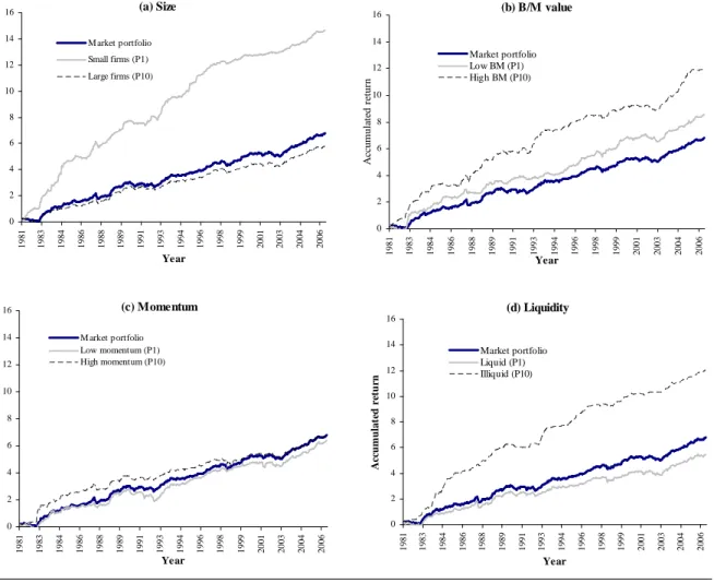
least liquid stocks would in 1980-2006 have given excess returns of more than 1.5% per month. This result seems consistent across subperiods. In panel B the table shows that the portfolio of least liquid stocks has had a systematically higher return than the most liquid companies. Also note that the dierence is not signicant in the last subperiod. To summarize the results of this subsection gure 4 illustrates the importance of the dierent anomalies. In each gure we compare three simple portfolio strategies (two extreme portfolios and the market portfolio). In each gure the extreme portfolios correspond to portfolio 1 and 10 in the preceding tables. The portfolios are value weighted using company market values. In gure 4(a) we show the accumulated return (without reinvestment) of a portfolio of the 10% smallest companies (grey line) and a portfolio of the 10% largest companies (broken line). These portfolios are reconstructed every year-end using company market values, and weights are kept constant through the year. In the gure the solid black line shows the accumulated return of the market index. Correspondingly, gure (b) shows results when we construct portfolios based on book to market values at the end of the year. Figure (c) shows the return of portfolios sorted on the previous year's return (momentum) and (d) shows results for portfolios based on relative spread (liquidity). Observe that in particular the size strategy (a) and liquidity strategy (d) give high excess returns relative to the market. Also the Book/Market strategy in (b) gives a positive excess return relative to the market, while the momentum strategy (c) does not give any excess return relative to the market. Figure 4 indicates that there is something special about particularly the size and liquidity portfolios which lead to excess returns. The excess return is however not adjusted for risk. In the next sections we will investigate whether there also is a risk-adjusted excess return related to the anomalies, and whether any such excess return can be explained by risk factors other than the market.

3.2 Method for estimation of factor models

In this subsection we give a short presentation of the methods of estimation used to test various valuation models. As mentioned in the introduction, in a theoretical factor model one will assume that the expected return for a stock in excess of the risk-free return in equilibrium can be expressed as

(23)

Figure 4 Portfolios based on various characteristics

The gures show the accumulated return (without reinvestment) for portfolios constructed at the beginning of each year based on (a) size, (b) book-to-market value (B/M), (c) momentum and (d) liquidity. In each gure we show the accumulated return for the two extreme portfolios for each characteristic in addition to the accumulated return on the value-weighted market portfolio. Note that the portfolio returns are not adjusted for market risk.

(b) B/M value 0 2 4 6 8 10 12 14 16 1 9 8 1 1 9 8 3 1 9 8 4 1 9 8 6 1 9 8 8 1 9 8 9 1 9 9 1 1 9 9 3 1 9 9 4 1 9 9 6 1 9 9 8 1 9 9 9 2 0 0 1 2 0 0 3 2 0 0 4 2 0 0 6 Year A cc u m u la te d r et u rn Market portfolio Low BM (P1) High BM (P10) (a) Size 0 2 4 6 8 10 12 14 16 1 9 8 1 1 9 8 3 1 9 8 4 1 9 8 6 1 9 8 8 1 9 8 9 1 9 9 1 1 9 9 3 1 9 9 4 1 9 9 6 1 9 9 8 1 9 9 9 2 0 0 1 2 0 0 3 2 0 0 4 2 0 0 6 Year A cc u m u la te d r et u rn M arket portfolio Small firms (P1) Large firms (P10) (d) Liquidity 0 2 4 6 8 10 12 14 16 1 9 8 1 1 9 8 3 1 9 8 4 1 9 8 6 1 9 8 8 1 9 8 9 1 9 9 1 1 9 9 3 1 9 9 4 1 9 9 6 1 9 9 8 1 9 9 9 2 0 0 1 2 0 0 3 2 0 0 4 2 0 0 6 Year A cc u m u la te d r et u rn Market portfolio Liquid (P1) Illiquid (P10) (c) Momentum 0 2 4 6 8 10 12 14 16 1 9 8 1 1 9 8 3 1 9 8 4 1 9 8 6 1 9 8 8 1 9 8 9 1 9 9 1 1 9 9 3 1 9 9 4 1 9 9 6 1 9 9 8 1 9 9 9 2 0 0 1 2 0 0 3 2 0 0 4 2 0 0 6 Year A cc u m u la te d r et u rn M arket p ortfolio Low momentum (P1) High momentum (P10)

(24)

where E[eri] is expected excess return for stock i, j ∈ {1, .., J} the number of factors

aecting returns, βi

j is the exposure to risk factor j for stock i and λj is the risk

premium for risk factor j common to the whole market.

There are various methods for estimating risk premia for one or more factors, and testing whether a model can price a collection of assets. The traditional method uses two steps. The rst step is the method developed by Black, Jensen, and Scholes (1972), time series regressions of the type

eri_t =ai+ J X j=1 βi_jfjt+εit (7) where eri

t is the excess return for stock i, ai a constant term, and βij the estimated

exposure to factorfj of stocki. The estimated factor exposures measure the sensitivity

of the return of an asset to movements in the respective factors. When a factor is expressed as a return series, for example as the return on a portfolio of large companies less the return on a portfolio of small companies, the factor model can be tested by testing the restriction that all the constant terms, ai_{, equal zero. If this is rejected the}

model is rejected. If a factor model includes factors which are not return series, such as ination or money stock, the analysis does not have such an interpretation.14

In this estimation we do not use the restriction of constant risk premia across assets. The next step in the the two-step procedure is therefore to estimate factor risk premia, and test whether the model is able to price stocks/portfolios correctly. Given the estimates from (7), the risk premium linked to factor j can be estimated by a

cross-sectional regression eri=λ0 + J X j=1 λjβij+ε i ₍₈₎

where λ0 is a constant term, and λj is the risk premium of factor j. Finally, we will

perform statistical tests on λj to investigate whether the risk premia of the various

factors are signicantly dierent from zero.

The traditional way of estimating (7) and (8) has been OLS. A problem with es-timation of the model in two steps using OLS is the \generated regressors" problem,

14_{If one wishes to do such a test it is necessary to construct so-called \mimicking portfolios"}

rep-resenting the factors. A \mimicking portfolio" is a portfolio of stocks with similar properties to the factor. A couple of well known such mimicking portfolios are the Fama/French factors based on return representation of size and B/M.

(25)

that is that one does not account for the explanatory variables (βi) in (8) having

es-timation errors. In newer literature it is becoming increasingly common to use the GMM (Generalized Method of Moments) method instead of this two-step procedure. By using GMM one can estimate (7) and (8) simultaneously, thereby accounting for the errors in variables problem. In addition, the GMM method is more robust to time series and distributional properties of the error terms.15

3.2.1 GMM estimation in a SDF setting

In newer empirical nance literature it is most common to do estimation by estimating the stochastic discount factor (SDF orm) directly. SDF estimation will give estimates

of the same risk premia as the above two-step procedure. The advantage of the SDF framework is that it is so general that it handles a number of dierent models. The framework is also particularly well suited in cases where the model contains factors which are not returns (such as macroeconomic variables). The SDF framework can incorporate such factors directly in the estimation, without the need for constructed \factor mimicking" portfolios. One problem with the direct SDF procedure is that it is less intuitive than the two-step procedure. The results from a SDF estimation also produce a bit less information.

The GMM method takes as its starting point a set of \moment conditions" derived from the underlying model to be estimated.16 _{The general pricing relationship in}

equation (4) in the introduction gives us the necessary moment conditions to identify valuation models in the SDF framework. Rewriting it in returns form we have that

Emterit

=0 (9)

This expression merely says that the risk-adjusted excess returns of all assets equal zero. It is necessary to put more structure on m to get a testable model. The SDF

framework is hence very general as the specication of m depends on the valuation

model employed. Since we in this study estimate and test unconditional linear factor

15_{If a model is estimated by OLS it is assumed that the error term is identically and independently}

distributed (iid). If the iid assumption is not valid, the OLS estimates will be biased with too low standard errors. GMM on the other hand will provide robust standard errors even in the non-iid case. In the special case of iid error term, the standard errors of the parameter estimates will be the same as in the case of OLS.

16_{The following is a short, intuitive summary of GMM estimation. For more detail we refer to Cochrane}

(26)

models we assume mt is a linear function of a set of risk factors and can be expressed as mt =c+ J X j=1 bjfj,t (10)

where c is a constant, bj the factor weight of risk factorfj, and we haveJ risk factors.

In this study we will estimate all models in the SDF framework with the GMM method. In most cases we will also estimate factor exposures as in (6), since this gives us additional information about how the return of for example sector portfolios co-vary with dierent factors (βi

j). GMM estimation proceeds by nding, for a given

set of assets (stock/portfolio returns) with excess returns eri_t and risk factors fj, the

factor weights bj that makes the moment condition (9) equal to zero.17 The GMM

procedure in other words nds the values of factor weights which set the vector of moment conditions for all the portfolios (pricing errors) simultaneously closest to zero. To evaluate the appropriateness of various factor models we use Hansen (1982)'s J-test. Suppose we have a cross-section of assets, and want to test a j -factor model. If n > j, which often is the case, the system is over-identied. The J test is used to

test whether the over-identifying moment conditions are close to zero. In this case the J-test will say something about the size of the pricing errors from the factor model, and thereby how well the model ts the data.

A factor weight (b) in (10) says something about how important the given factor

is in pricing the portfolios, given the other factors. These factor weights should not be mistaken for the β estimates from (7). After having estimated b we calculate the

risk premia λ as λj = −var(fj)bj. By testing whether the risk premia of the various

factors equal zero, we can investigate whether a factor is priced. For factors which are returns (for example the market factor) λ gives a direct estimate of how much extra

excess return one unit of extra exposure to the factor gives. For factors which are not return-based, one can not directly see from estimates ofλthe implications for expected

excess returns.

3.3 Capital Asset Pricing Model (CAPM)

The CAPM formalizes, in a simple way, the idea that the expected return on an asset should be higher the more risky the asset is. The model is based on very simplied

(27)

assumptions, where for example investors live for only one period, and have no other income. The model's assumptions lead to the only relevant risk for an asset being given by the asset's covariance with a value-weighted portfolio of all assets in the economy (the market portfolio). The CAPM can therefore be viewed as a special case of (6), where the market portfolio is the only relevant risk factor. To test the CAPM we need a proxy for the market portfolio.

What market portfolio to use in tests of the CAPM is much discussed in empirical nance. A well known article by Roll (1977) points out that the theoretically correct market portfolio, the portfolio of all assets in the economy, is unobservable, and a wrong proxy can give wrong conclusions. Even if this is acknowledged as a problem, newer literature has settled on using a wide stock market portfolio as a proxy for the market portfolio. It has also been found that for single country analyses one should use a broad market index for the market in question. For the Norwegian market a value weighted market portfolio will however mainly reect the return of a few large companies (see table 4). We therefore estimate all specications of models using both value and equally weighted market portfolios.

To reduce noise in estimation it is common to test factor models at the portfolio level. The CAPM predicts that companies with high market beta have high returns. To test this prediction it is sensible that the portfolio betas have a good cross-sectional distribution. It is therefore usual to sort portfolios using stock beta.18 _{To investigate}

to what extent the CAPM prices stocks within the various industry sectors we also use industry sectors as a basis for portfolio sorts.

3.3.1 CAPM using a market index at the OSE

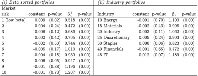
In this section we report results from estimating the CAPM where we use the market index at the OSE as a proxy for the market portfolio. Panel A in table 10 shows results from estimation of the CAPM for portfolios sorted on beta and industry. Both the beta and industry portfolios are value weighted. However, we nd similar results for equally weighted portfolios. Note that we only have sucient data for 7 of the 10 industry sectors. The calculations are based on monthly gures for the period 1982-2006.19

Columns two and three for each portfolio sort in panel A show estimated constant

18_{The beta portfolios are constructed at the end of each year and held constant through the following}

year. Market beta for each stock is estimated using returns data for the three previous years.

(28)

terms with accompanying p-values for each portfolio (industry sector). Constant terms signicantly dierent from zero indicate a badly specied model. The last two columns in each portfolio sort show estimated market betas (β1

i) and accompanying p values for

each portfolio (industry) for an equally-weighted market portfolio. Estimated exposures using a value-weighted portfolio are not signicantly dierent. Exposures are calculated using a time series regression as in (7). Panel B in the table shows the estimated risk premium,λ, for the market factor (equally weighted and value weighted) and the result

of a J-test for for the explanatory power of the model.20 _{A factor is said to be priced}

if λis signicantly dierent from zero. The J-test is based on the pricing errors of the

model. A low p-value for this test suggests that the model should be rejected. The estimated risk premia are estimated using GMM in a SDF framework, as described in section 3.2.1.

Both models give signicant betas for all portfolios. For the beta-sorted portfolios beta varies from 0.63 for portfolio 1 to 1.29 for portfolio 10. The betas of the industry portfolios also have a reasonable distribution, where the energy sector has the highest risk as measured by beta, and the nancial sector the lowest beta. For the industry-sorted portfolios estimated risk premia are dierent from zero independently of whether we use an equally- or value-weighted market portfolio. For the beta-sorted portfolios only the equally weighted market portfolio results in a signicant risk premium. None of the models has a constant term dierent from zero at the 1 % level. The models can neither be rejected based on the p-values of the J-tests. We nd that the market portfolio is a priced risk factor, and that the CAPM is a reasonably well specied model for portfolios sorted on market risk and industry sector.

We then move to anomalies relative to the CAPM. Tables 11 and 12 show results of estimation of the CAPM on portfolios sorted on the various anomalies. All portfolio sorts in the tables are value weighted. Results for equally weighted portfolios sorts are similar.

Table 11 shows results from an estimation using size portfolios and an estimation using liquidity portfolios. We see that the beta estimates are signicant for all portfolios in both models. The cross-sectional dierence in estimated betas is however low. In spite of this we nd that the market portfolio is a priced risk factor in all models with one exception: a value-weighted market portfolio and size-sorted portfolios. All size portfolios except the two containing the largest companies (portfolios 9 and 10) have

(29)

Table 10 Estimation of the CAPM on portfolios sorted on market beta and industry

sector

Panel A shows the results from estimating the CAPM as in equation (7) for portfolios sorted on market beta (i) and industry sectors (ii). Both the beta- and industry-portfolios are value weighted. For each set of portfolios, columns two and three show the estimated constant with the associated p-value for each portfolio. Constants that are signicantly dierent from zero indicate a wrongly specied model. The

last two columns for each set of portfolios show the estimated market beta (β1

i) and associated p-value.

Panel B shows the risk-premia estimated in the SDF framework using GMM as described in section

3.2.1. The risk premium, λ, is estimated both using an equally-weighted (erew

m ) and value-weighted

(ervwm ) market portfolio. A factor is said to be priced if λis signicantly dierent from zero. Panel B

also reports the results of a J-test of the models. The J-test is based on the size of the pricing errors of the model. A low p-value indicates a rejection of the model.

Panel A:Exposure estimates

(i) Beta sorted portfolios (ii) Industry portfolios

Market

risk constant p-value β1_i p-value Industry constant p-value βi p-value

1 (low beta) 0.009 (0.02) 0.518 (0.00) 10 Energy -0.001 (0.70) 1.103 (0.00)

2 0.004 (0.24) 0.472 (0.00) 15 Materials -0.002 (0.43) 0.998 (0.00) 3 0.006 (0.12) 0.686 (0.00) 20 Industry -0.003 (0.11) 1.062 (0.00) 4 0.002 (0.42) 0.705 (0.00) 25 Discretionary 0.005 (0.24) 0.903 (0.00) 5 -0.002 (0.50) 0.744 (0.00) 30 Staples 0.006 (0.06) 0.823 (0.00) 6 -0.005 (0.17) 1.010 (0.00) 40 Financials -0.001 (0.65) 0.772 (0.00) 7 -0.004 (0.18) 0.939 (0.00) 45 IT 0.012 (0.07) 1.189 (0.00) 8 -0.006 (0.05) 0.947 (0.00) 9 -0.001 (0.88) 1.196 (0.00) 10 -0.001 (0.73) 1.207 (0.00)

Panel B:Risk-premia estimates

(i) Beta sorted portfolios (ii) Industry portfolios

Risk Risk

Factor premium t-value Factor premium t-value

λ[1](erew

m ) 0.014 (2.70) λ[1](erewm ) 0.014 (2.97)

λ[1](ervw

m ) 0.001 (1.92) λ[1](ervwm ) 0.015 (3.07)

Chi Square test J (χ2₍₉₎_{) p-value} _{J (}_χ2₍₆₎_{) p-value}

erew_m 6.22 (0.51) erew_m 5.57 (0.23)

ervw

(30)

Table 11 Estimation of the CAPM on portfolios sorted on size and relative spread

Panel A shows the results from estimating the CAPM as in equation 7 for portfolios sorted on size (i) and liquidity (ii). Firm size is measured as the market capitalization and liquidity is measured by the rms' relative spread. Both the size- and liquidity portfolios are value weighted. For each set of portfolios, columns two and three show the estimated constant with the associated p-value for each portfolio. Constants that are signicantly dierent from zero indicate a wrongly specied model. The

two last columns for each set of portfolios show the estimated market beta (β1

3.2.1. The risk premium, λ, is estimated both using an equally weighted (erew

(ervwm ) market portfolio. A factor is said to be priced if λis signicantly dierent from zero. Panel B

Size portfolios Liquidity portfolios

Size constant p-value β1

i p-value Liquidity constant p-value β1i p-value

1 (low MCAP) 0.037 (0.00) 0.674 (0.00) 1 (low spread) -0.005 (0.00) 1.017 (0.00)

2 0.027 (0.00) 0.621 (0.00) 2 -0.002 (0.35) 1.020 (0.00) 3 0.010 (0.01) 0.851 (0.00) 3 0.001 (0.61) 1.087 (0.00) 4 0.015 (0.00) 0.827 (0.00) 4 0.003 (0.33) 1.001 (0.00) 5 0.014 (0.00) 0.792 (0.00) 5 0.003 (0.20) 0.869 (0.00) 6 0.013 (0.00) 0.875 (0.00) 6 0.004 (0.19) 0.895 (0.00) 7 0.008 (0.01) 0.871 (0.00) 7 0.005 (0.14) 0.905 (0.00) 8 0.007 (0.01) 0.931 (0.00) 8 0.013 (0.00) 0.787 (0.00) 9 0.001 (0.73) 1.035 (0.00) 9 0.016 (0.00) 0.752 (0.00) 10 -0.004 (0.00) 1.022 (0.00) 10 0.025 (0.00) 0.669 (0.00)

Size portfolios Liquidity portfolios

Risk Risk

λ[1](erew

m ) 0.026 (5.73) λ[1](erewm ) 0.026 (5.36)

λ[1](ervwm ) 0.008 (1.90) λ[1](ervwm ) 0.018 (3.48)

Chi Square test J (χ2(9)) p-value J (χ2(6)) p-value

erew

m 20.01 (0.01) erewm 20.71 (0.00)

ervw

(31)

however constant terms signicantly dierent from zero. The portfolios with lowest liquidity (as measured by relative spread) also have signicant constant terms. Also note that the constant term is increasing in size and increasing liquidity (falling spread). The J-test is signicantly dierent from zero at the 1 % level for both the size portfolios and the liquidity portfolios, suggesting that the pricing errors from the various models are large. The CAPM does not seem able to price neither size portfolios or the liquidity portfolios. This indicates a size eect in the Norwegian market, related to liquidity.

Table 12 shows results from estimations where we sort portfolios on book val-ues/market values (B/M) and momentum. We nd signicant beta estimates, a nice spread in portfolio betas, and signicant risk premia in both models. Portfolios with lowest B/M and highest B/M have constant terms signicantly dierent from zero at respectively the 2 % and 1 % level. The model is also rejected by the p-value of the J-test. The momentum model is however not rejected by the p-value of the J-test. CAPM seems in other words to price momentum portfolios well. We therefore have only weak signs of momentum eects in the Norwegian equity market.

3.4 Multi-factor models based on empirically constructed

fac-tors

A common trait of the multi-factor models ICAPM and APT is that they do not identify what factors are important for returns. According to the ICAPM, stock returns will be driven by the market factor of the CAPM together with all factors (or state variables) important for the conditional distribution of future returns. In the APT model the common factors are estimated statistically using the returns on all assets in the market. To support the APT a signicant factor should also be important for realized returns. This is not necessarily the case for an ICAPM factor. An advantage of the ICAPM model is the ability to apply theory to suggest candidate factors.

In table 11 we show that the market factor in the CAPM is unable to price portfolios sorted on size and liquidity. This is strong evidence that the CAPM is not sucient to explain the Norwegian market. In the framework of a multi-factor model this can be explained by size and liquidity being risk factors for which investors demand compen-sation to be exposed to, but which are not expressed in the market portfolio. In this section we construct risk factors from the CAPM anomalies, and test to what extent this type of multi-factor model explains asset returns better in the Norwegian market,

(32)

Table 12 Estimation of the CAPM on portfolios sorted on B/M and momentum

Panel A shows the results from estimating the CAPM as in equation (7) for portfolios sorted on B/M-value (i) and momentum (ii). Both the size- and liquidity portfolios are B/M-value weighted. For each set of portfolios, columns two and three show the estimated constant with the associated p-value for each portfolio. Constants that are signicantly dierent from zero indicate a wrongly specied model. The

two last columns for each set of portfolios show the estimated market beta (β1

3.2.1. The risk premium, λ, is estimated both using an equally-weighted (erew

(ervw_m ) market portfolio. A factor is said to be priced if λis signicantly dierent from zero. Panel B

B/M portfolios Momentum portfolios

B/M constant p-value β1 p-value Momentum constant p-value β1 p-value

1 (low B/M) 0.006 (0.15) 0.964 (0.00) 1 (low momentum) -0.001 (0.77) 0.973 (0.00)

2 0.004 (0.39) 0.902 (0.00) 2 0.001 (0.66) 0.966 (0.00) 3 -0.007 (0.03) 1.006 (0.00) 3 0.001 (0.86) 1.052 (0.00) 4 -0.003 (0.29) 0.988 (0.00) 4 -0.003 (0.54) 1.049 (0.00) 5 0.001 (0.66) 1.018 (0.00) 5 0.014 (0.00) 0.962 (0.00) 6 -0.001 (0.91) 1.042 (0.00) 6 -0.004 (0.25) 0.846 (0.00) 7 0.004 (0.21) 1.115 (0.00) 7 0.002 (0.47) 0.788 (0.00) 8 0.003 (0.32) 1.061 (0.00) 8 -0.001 (0.87) 1.012 (0.00) 9 0.005 (0.21) 1.173 (0.00) 9 0.003 (0.31) 0.907 (0.00) 10 0.017 (0.00) 0.992 (0.00) 10 0.004 (0.19) 1.026 (0.00)

B/M portfolios Momentum portfolios

Risk Risk

λ[1](erew

m ) 0.014 (3.04) λ[1](erewm ) 0.014 (2.96)

λ[1](ervw_m ) 0.012 (2.62) λ[1](ervw_m ) 0.015 (3.13)

Chi Square test J (χ2(9)) p-value J (χ2(6)) p-value

erew

m 16.76 (0.02) erewm 11.24 (0.13)

(33)

relative to a single market factor. All risk factors are estimated using stocks at the Oslo Stock Exchange.

The three-factor model developed by Fama and French (1992, 1993) contains in addition to the market factor a factor HML (\high minus low") designed to measure

the B/M eect, and a factor SMB (\small minus big") based on rm size. HML is a

portfolio containing long positions in companies with high B/M and short positions in companies with low B/M. Similarly SMB is a portfolio of long positions in small

companies and short positions in large companies. Both HML and SMB are constructed

as zero investment portfolios. It is important to emphasize that these portfolios are constructed ex-ante using available information about characteristics of the companies at the time of construction. In other words they are implementable trading strategies. Specically, the factors are constructed as follows. First companies at the OSE are sorted into three B/M portfolios (H,M,L). Thereafter companies in each B/M portfolio are sorted into two size portfolios (S,B). Finally, HMLandSMB are constructed from the

size cross-sorted portfolios (SH,SM,SL,BH,BM,BL) in such a manner that they are zero investments: HML= 1 2SH+ 1 2BH − 1 2SL+ 1 2BL (11) SMB= 1 3SH+ 1 3SM+ 1 3SL − 1 3BH+ 1 3BM+ 1 3BL (12) Carhart (1997) expands on the three-factor model by adding an additional factor (PR1YR) based on the momentum eect, identied by Jegadeesh and Titman (1993), in

order to explain persistence in the returns of US mutual funds. PR1YR is constructed

by sorting companies into 3 portfolios at the end of each month, based on the asset returns over the preceding 11 months. These portfolios are held constant through the month, before they are regrouped at the end of the month. ThePR1YR risk factor is the

dierence between returns of portfolios 3 and 1. Another momentum factor much used in the literature is UMD (\Up minus Down"). The UMD factor is based on a cross-sort

similar to the Fama and French factors. The main dierence between UMD and PR1YR

is that UMD attempts to correct for the size eect.

In table 13 we show results from an estimation of a four-factor model consisting of the Fama and French factors (Rm, SMB, HML) and the momentum factor (UMD). The

table shows that four out of seven industry sectors have a signicant exposure to the